Atrous Pyramid GAN Segmentation Network for Fish Images with High Performance

Abstract

With the development of computer science technology, theory and method of image segmentation are widely used in fish discrimination, which plays an important role in improving the efficiency of fisheries sorting and biodiversity studying. However, the existing methods of fish images segmentation are less accurate and inefficient, which is worthy of in-depth exploration. Therefore, this paper proposes an atrous pyramid GAN segmentation network aimed at increasing accuracy and efficiency. This paper introduces an atrous pyramid structure, and the GAN module is added before the CNN backbone in order to augment the dataset. The Atrous pyramid structure first fuses the input and output of the dilated convolutional layer with a small sampling rate and then feeds the fused features into the subsequent dilated convolutional layer with a large sampling rate to obtain dense multiscale contextual information. Thus, by capturing richer contextual information, this structure improves the accuracy of segmentation results. In addition to the aforementioned innovation, various data enhancement methods, such as MixUp, Mosaic, CutMix, and CutOut, are used in this paper to enhance the model’s robustness. This paper also improves the loss function and uses the label smoothing method to prevent model overfitting. The improvement is also tested by extensive ablation experiments. As a result, our model’s F1-score, GA, and MIoU were tested on the validation dataset, reaching 0.961, 0.981, and 0.973, respectively. This experimental result demonstrates that the proposed model outperforms all the other contrast models. Moreover, in order to accelerate the deployment of the encapsulated model on hardware, this paper optimizes the execution time of the matrix multiplication method on Hbird E203 based on Strassen’s algorithm to ensure the efficient operation of the model on this hardware platform.

1. Introduction

Fish is an important aquatic organism that is widely distributed in the world. Fish was one of the earliest protein source for people in ancient times [1]. Recent studies have shown that there are approximately 27,683 species of fish in the world, divided into 6 classes, 62 orders, and 540 families [2,3]. Mora et al. found that globally, among all marine fish species, approximately 21% remain to be described [4]. The huge number of species and the rich genetic characteristics impose a heavy burden on the study of life diversity, which is the basis of all biological research. Therefore, the taxonomic identification of species is a challenge.

Rapid species identification of fish plays an important role in the fisheries industry. Rapid fish sorting can effectively improve the efficiency of fisheries and reduce the workload of staff, which is an important basis for fisheries resource management and drives the world’s fisheries into standardization, digitalization, and industrialization. Additionally, fish identification is helpful for water environmental management. Researchers determine the trajectory of fish in a specific water quality environment through the vision, obtain the parameters of movement by analyzing the swimming trajectory of fish, and build a water quality safety evaluation model. By inputting the swimming trajectories of different fish under different water quality into the model, the user can easily judge the water environment. Based on this, the water environment could be continuously monitored and be effectively managed, which will be helpful in achieving the sustainable exploitation of marine natural resources [5,6].

With the rapid development of fishery and the increase in requirements for the accuracy of fish species classification, there is an urgent need for fish species discrimination methods. For traditional fish segmentation and classification methods, morphological characters remain the standard and cornerstone of taxonomic treatment. Morphology-based identification systems have successfully described nearly one million species of fish on earth, providing a good basis for fish taxonomic identification [7]. However, there are several drawbacks of morphological identification-based fish classification methods:

• Marine organisms have an extraordinary diversity of colors, sizes, and shapes. Differences in epistatic traits and genetic variation for fish identification can lead to misclassification due to individual, sex, and geographic differences [8].
• Marine organisms exhibit different characteristics and morphology at different developmental stages, and species identification only by morphological traits alone is very difficult, even for trained experts [9,10].
• Large-scale fisheries surveys increase complexity and may require more number of experts to identify specimens from only a single sample collection, and the cost of collection and manpower required is high. Furthermore, efficiency classification only with morphological characters cannot be achieved by manual identification, which can be challenging and time consuming.
• Marine fish identification requires not only specialized taxonomic and systematic knowledge but also experience and knowledge of marine ecology, biogeography, and fishery management, which makes classification highly susceptible to errors [11].

The aforementioned problems often hinder the assessment and management of global fish biodiversity, which has prompted research more accurate methods of fish identification.

With the development of artificial intelligence for machine learning-based methods [12,13,14,15,16], the traditional convolutional neural network (CNN) has a powerful feature extraction capability compared with the traditional manual morphological recognition or the more complex operation of DNA barcode extraction methods. Deep learning and neural networks have been widely developed in the field of computer vision, which has made a large number of discoveries and achievements. Today, CNN-based target detection has surpassed traditional target detection methods and has become the mainstream of current target detection. Although the ability to automatically extract features has enabled deep learning to achieve satisfactory results in image segmentation tasks, image semantic segmentation is pixel-level, and the image details become progressively smaller in feature map size during convolution and pooling. Thus, it is impossible to achieve accurate segmentation without pointing out which object each pixel belongs to [17]. In order to make CNN better applied to image segmentation tasks, researchers have proposed different approaches.

With sufficiently large training data, Konovalov et al. trained an advanced CNN as the desired image classifier and, in practice, continuously finetuned CNN to obtain better recognition results, while image cleaning preprocessing is not necessary and could be detrimental to the CNN performance [18]. If there is no sufficient dataset during training, overfitting problems may occur in deep learning. To tackle this problem, Lee et al. used the dropout algorithm to simplify the model [19]. Štefanič et al. presented a new concept for engineering complex adaptable cloud systems with time-critical constraints: the application-infrastructure co-programming model, which offered application scalability, availability, resilience, and self-adaptation [20]. When the training dataset was derived from a digital camera, Cui et al. used three optimized methods for CNN, data augmentation, network simplification, and training process acceleration, composing a promising model which can be extended to the detection of other underwater organisms [21]. Schwartz et al. suggested a method of meta-algorithm (Mask R-CNN), which their fish segmentation model relies on, and it is well suited for generating high-fidelity segmented specimen images across a variety of background contexts at rapid pace [22]. Majumder et al. used six CNN-based transfer learning architectures, namely DenseNet201, InceptionResnetV2, InceptionV3, ResNet50, ResNet152V2, and Xception, to calculate Accuracy, Precision, Recall, and F1 scores. The methods of InceptionResnetV2 and Xception achieved the highest accuracy of 98.81% [23].

U-Net [24] is one of the most famous frameworks for segmentation. By automatic segmentation, image features can be learned automatically. Currently, many new design methods of convolutional neural networks are based on the core idea of U-Net and combine with new modules for innovation and improvement. Zhou et al. introduced nested and dense jump connections of U-Net, enhanced the connection between encoder and decoder, and proposed U-Net++ [25]. With the wide application of U-Net networks, U-Net was combined with other modules to obtain a large number of U-Net-based networks. Saleh et al. proposed a scheme based on U-Net and fish morphological features for accurate segmentation and measurement of tilted fish features [26].

In addition, for target fish that have small pixel areas, Labao et al. used the automatic correction mechanism in the cascaded ensemble structure of deep networks to improve the localization accuracy [27]. The ensemble structure can also be extended to the detection of other objects. Miyazono et al. proposed a new feature point representation method named annotated images to optimize the CNN-based fish species recognition method, which proved to be efficient in recognition accuracy by collecting images of 50 species of fish samples [28]. To face the challenges such as different specimens, rotations, positions, illuminations, and backgrounds existing in fish images, Ibrahima et al. built a segmentation model for fish images segmentations using the Salp Swarm Algorithm (SSA). The model shows robustness for different cases compared to conventional work [29]. For target fish that have almost the same appearances and frequently overlap, Wang et al. proposed an effective tracking method, by which fish heads were detected firstly with a scalar spatial method; then, the head image pattern of each fish in each frame was recognized to achieve the cross-frame data association. Finally, the prediction of the motion state and the recognition result by CNN were combined to associate detections across frames. The proposed method outperforms two state-of-the-art fish tracking methods in terms of P, R, F1, MT, ML, Frag, and IDS performance metrics [30].

In the process of image segmentation, the category information of pixel points has a certain possibility of correlation with the surrounding pixel points, but the category correlation between neighbouring pixel points is easily ignored when performing pixel by pixel classification, resulting in a lack of contextual information. Therefore, richer contextual information is beneficial to improve the segmentation accuracy of the model.

In the view of above, the paper proposes a convolutional dense pyramid pooling approach with generative modules to achieve a more accurate segmentation of fish images. Atrous Spatial Pyramid Pooling(ASPP), which was proposed by Chen et al. in 2017 [31], uses multiple cavity convolution to achieve segmentation of objects at different scales on an image by increasing the receptive field of the feature map. However, it fails to fully capture the contextual information contained between image pixel points. The segmentation algorithm proposed in this paper is optimized and improved based on the ASPP algorithm by adding densely connected convolutional networks, convolutional dense pyramid pooling, and generative modules to obtain the missing contextual information in the segmentation process, which in turn captures more multiscale contextual information and further improves segmentation accuracy for the objects of different scales presented in the image.

The remainder of this paper is arranged as follows: Section 2 introduces the development status of segmentation network. Section 3 introduces the dataset and describes our fish segmentation network in detail. Section 4 explains the experimental setup and evaluation indicators. Section 5 discusses validation and detection results and analyzes these experimental results. Section 6 conducts numerous ablation experiments to verify the efficacy of the optimized method. Section 7 is a summary of the entire paper.

2. Related Work

Image semantic segmentation is one of the research hotspots in the field of computer vision and an important part of image content analysis and understanding. It plays an important role in applications such as autonomous driving and medical image diagnosis. Thampi et al. also made outstanding progress in fish image segmentation using computer vision [32].

The CNN is essentially a feed-forward neural grid with convolution, which has an excellent performance in image processing. Compared with the traditional neural grid using a fully connected form, CNN uses local connections and weight sharing to greatly reduce the complexity of the model and reduce the number of parameters, thus decreasing the difficulty of model training. Local connectivity means that each neuron in each layer is connected only to the adjacent neuron in the previous layer, while full connectivity is connected to all neurons in the previous layer. Weight sharing means that each convolutional kernel in the convolutional layer has the same weight and bias parameters. CNN is also invariant in the sense that the corresponding features can be extracted after spatial transformations such as translation and scaling of the image. In addition to the input and output layers, CNN structure also includes a convolutional layer, a pooling layer, and a fully connected layer.

The most important component that carefully constitutes the convolutional layer in a CNN is the convolutional kernel, and each convolutional layer contains multiple trainable convolutional kernels. Convolutional kernels are featured extractors that can automatically extract features from incoming image data. The feature information extracted differs depending on the size of the convolution kernel used. The result of the convolution operation is then subjected to an activation function to obtain the output of the convolution layer. This is conducted to impose a nonlinear factor on the convolution result and to improve the model’s ability to represent the features. Low-level convolutional layers can only extract low-level feature information such as edges or curves, while high-level convolutional layers can extract abstract feature information with more complex relationships. The expression of convolutional layers is as follows.

$$c_j^l=\sum _{}{x}_i^l\otimes k_{ij}^l+b_j^l$$

(1)

$$x_j^{l+1}=y_j^l=f\left(c_j^l\right)$$

(2)

In Formulas (1) and (2), $c_j^l$ denotes the feature map created by the convolution operation of the jth feature map in the lth layer, $x_i^l$ denotes the ith input feature map in the lth layer, $k_{ij}^l$ denotes the ith feature map in the lth layer and the convolution kernel of the jth feature map, ⊗ denotes the convolution operation, $b_j^l$ denotes the bias term in the lth layer, $f\left(\right)$ and $y_j^l$ denote the activation function in the lth layer and the jth output feature map, respectively, and $x_j^{l+1}$ denotes the jth input feature map in the $l+1$th layer.

The pooling layer is called the downsampling layer, which is closely behind the convolution layer. The principle of the pooling layer is as follows: firstly, the feature map is chunked, then shifted according to a set step, and the maximum or average pixel value within each chunk is calculated. For the pooling layer, on the one hand, it reduces the computational effort and speeds up training by reducing the dimensionality of the high-dimensional features obtained from the convolutional layer while retaining useful feature information. On the other hand, the pooling layer also makes the network spatially invariant. The output of the pooling layer depends on the size of the input feature map, the size of the pooling kernel, and the number of moves. Common pooling methods include maximum pooling, which takes the maximum value of the local features, and average pooling, which takes the average value of the local features.

Fully connected layers: After multiple convolutional and pooling layers, several more fully connected layers are connected at the end of the grid, and the layers are connected in a fully connected form. The layers are connected in a fully connected manner. The fully connected layer transforms the resulting two-dimensional feature map into a one-dimensional feature vector. The purpose is to obtain global features by combining all local features so that the subsequent output layers can be used for classification calculations. ReLU [33] is the most commonly used activation function in this layer.

In a classical CNN, the input of the fully connected layer must have a fixed length; thus, the input image of the network must also have a fixed size. However, in practice, the majority of the network input images are not sufficiently large to meet the input size requirement. The traditional solution is to transform the image size to a fixed size using crop or warp operations, but these methods may distort input images. Spatial pyramid pooling can divide the image into blocks of different sizes without crop and warp operations and then aggregate these blocks to transform them into the input size required by the fully connected layer.

Suppose an image of arbitrary size is used as the input of a grid by using the spatial metallic pooling technique, as observed from Figure 1, we can slice this image into three different scales, with the scale size of 4 × 4, 2 × 2, and 1 × 1, so that the image blocks are 16, 4, and 1, respectively. Then, the maximum pooling operation is performed on these 21 blocks, and each block can obtain a pooling feature. Finally, all the pooled features obtained are spliced to obtain the input features of fixed dimensions that meet the requirements of the full connection layer, which is obtained the required 21-dimensional feature vectors.

In summary, the advantages of spatial pyramid pooling include the following: first, the size of the image input to the network can be changed from a fixed size to an arbitrary size; second, feature extraction is performed from different scales to obtain more contextual information.

The segmentation method based on CNN can only achieve the semantic segmentation of image content at the image level; thus, its segmentation accuracy is low. Zhou et al. made a breakthrough in the field of cross-image pixel contrast for semantic segmentation, weakly supervised semantic segmentation, and video object segmentation [34,35,36]. Moreover, the fully convolutional network(FCN) [37] can perform end-to-end pixel-level semantic segmentation of image content, which greatly improves the accuracy of semantic segmentation. Since then, the network architecture used for image semantic segmentation has been derived from FCN, which has become the pioneer of pixel-level image semantic segmentation.

The design idea of the FCN is relatively simple and consists of two major innovations:

• The use of convolutional layers instead of fully connected layers. The FCN is based on the CNN with the last part of the structure modified, i.e., the first five components remain unchanged, but the last three fully connected layers are replaced by convolutional layers. The last three fully connected layers in the CNN are all one-dimensional vectors with lengths of 4096, 4096, and 1000, respectively. Instead, the three fully connected layers in the FCN network are replaced with convolutional layers, and the corresponding one-dimensional vectors are converted into tensors, which are $(4096,1,1)$, $(4096,1,1)$, and $(1000,1,1)$, where each number in parentheses represents the number of channels, width, and height, respectively. Since all layers in the grid are convolutional, the new grid structure is called the fully convolutional neural grid.
• Multilevel fusion using upsampling and jump connections. As multiple convolutions and pooling operations are used, the resolution of the feature map gradually decreases by a factor of 2, 4, 8, 16, and 32. If a feature map with a size of $\frac{1}{32}$ of the original input image is directly segmented semantically, a large number of spatial information will be lost due to the low resolution of the feature map, resulting in poor segmentation results. Therefore, FCN uses upsampling to expand the feature map resolution. In addition, the FCN considers that if only the output feature map of the last layer ($\frac{1}{32}$ of the size of the original input image) is upsampled with a sampling factor of 32, a feature map of the same size as the original input image is obtained, but this will also result in unsatisfactory segmentation results. For this reason, FCN introduces a jump connection, which uses upsampling to expand the feature map at the last layer (conv7) by a factor of two, and then uses the jump connection to fuse the expanded feature map with the feature map obtained at the pool4 stage to obtain a feature map with a size of $\frac{1}{16}$. Next, the $\frac{1}{16}$th feature map is upsampled by a factor of two and fused with the pool3 feature map using a jump connection to obtain a feature map with a size of $\frac{1}{8}$th. After the multi-stage fusion process is completed, FCN upsamples the last fused feature map (of size $\frac{1}{8}$) by a factor of 8 to achieve end-to-end pixel-level semantic segmentation.

The advantages of the image semantic segmentation method based on FCN include the following:

• No limitation on the size of the input image;
• Higher efficiency by avoiding repeated computations and wasted storage space.

3. Materials and Methods

This dataset that we used in this paper contains 9 different seafood types collected from a supermarket, and this work was published in ASYU 2020 [38]. This dataset includes, gilt head bream, red sea bream, sea bass, red mullet, horse mackerel, black sea sprat, striped red mullet, trout, and shrimp image samples, as shown in Figure 2.

All images in this dataset were collected via two different cameras: Kodak Easyshare Z650 and Samsung ST60. Therefore, the resolution of the images are $2832\times 2128$ and $1024\times 768$, respectively. Before the segmentation, feature extraction, and classification process, the dataset was resized to $590\times 445$ by preserving the aspect ratio. After resizing the images, all labels in the dataset were augmented by flipping and rotating. At the end of the augmentation process, the number of total images for each class became 2000: 1000 for the RGB fish images and 1000 for their pair-wise ground truth labels.

3.1. Dataset Analysis

As shown in Figure 2, in this paper, the dataset has following features:

• The dataset contains many kinds of fish, some of which are very close in appearances such as the Black Sea Sprat and Hourse Mackerel;
• Uneven distribution of samples in the dataset;
• The overall amount of data is small, which makes deep learning training very difficult.

3.2. Data Enhancement

3.2.1. Basic Enhancement

This paper referred to the method proposed by Alex et al. [33], by using image flipping, translation, etc. These methods mainly improve the model’s accuracy by increasing the amount of images. The main purpose of image scaling is to improve the robustness of the model for the same object at different scales. The scales of different objects are different; thus, it is necessary to improve the ability of the model to detect the same object at different scales.

In addition to those mentioned above, spatial and scale data enhancements with fundamental, color-channel transformations, such as HSV channel color variations, are used in this paper to enhance the recognition accuracy of our model in different lighting conditions.

3.2.2. Advanced Enhancement

In order to further enrich the number of images in the dataset, the following data enhancement methods are also applied.

The Mixup [39] neighborhood distribution can be understood as a form of data augmentation that causes the model to behave linearly when dealing with the region between samples and samples. We believe that this form of linear modeling reduces maladjustments in predicting data outside of the training sample. Starting from the principle of Occam’s razor, linearity is a good generalization bias because it is one of the simplest possible several behaviors.

Mosaic [40] data enhancement, this data enhancement method simply takes four images and stitches them together by random scaling, random cropping, and random lining up. The advantage of this method is that it enriches the background of the detected objects and small targets, and it calculates the data of four images at a time when calculating Batch Normalization, which allows the mini-batch size to not be as large, and a GPU can achieve better results.

The starting point of Cutout [41] is the same as Random Erasing, which also simulates occlusion and aims to improve generalization ability. The implementation is simpler than Random Erasing, which randomly selects a square region of fixed size and then uses all-0 filling. In order to avoid the impact of filling 0 values on training, the data should be subjected to a central normalization operation: norm to 0.

The CutMix [42] operation enables the model to identify two targets from a local view on an image, improving training efficiency. Cutmix can make full use of all pixel information, but it may introduce some unnatural pseudo-pixel information. The operation of CutMix can be expressed by the Formulas (3) and (4).

$$\overline{x}=M\odot x_A+(1-M)\odot x_B$$

(3)

$$\overline{y}=\lambda \times y_A+(1-\lambda )\times y_B$$

(4)

M is a binary Mask. For $x_A$, the $M=1$ part of the image is preserved. $x_B$, the $M=0$ part of the image is preserved; $x_A$ and $x_B$ are the two images respectively, and $y_A$ and $y_B$ are the corresponding labels respectively; $\overline{x}$ and $\overline{y}$ are the images after CutMix; ⊙ means multiply by elements; and $\lambda$ obeys $\beta (\alpha ,\alpha )$ distribution. The value of M is obtained by randomly generating a bounding box, the size of the M matrix is the same as the input image, and the values inside the bounding box are 0 and the other values are 1. The percentage of the current image content in the fused area determines the value of the label. Suppose the original labels are $[1,0]$ and $[0,1]$ with 30% and 70% of the two images fused, respectively, then the fused labels are $[0.3,0.7]$.

These specific effects are shown in Figure 3.

3.2.3. Removal of Useless Details

Considering the characteristics of the dataset in this paper, for example, fish images contain a large amount of texture details; in order to reduce the interference of these non-essential details on the feature extraction ability of the model, a morphological method [43] was used to preprocess the images in this paper. First, the erosion operation is performed, and its logical procedure is shown in Formula (5). Although details can be removed by the erosion operation, the necessary classification features are also eliminated. Therefore, it is necessary to perform the dilation operation, for which its logical procedure is shown in Formula (6).

$$\alpha \odot \beta =\left\{z\right|{\left(\widehat{\beta }\right)}_z\subseteq \alpha \}$$

(5)

$$\alpha \oplus \beta =\left\{z\right|{\left(\widehat{\beta }\right)}_z\cap \alpha \ne \varnothing \}$$

(6)

In Formulas (5) and (6), $\alpha$ denotes image, and $\beta$ denotes the operator. The features of fish can be restored by dilation process. Figure 4 illustrates the visualization process of the method.

3.3. Atrous Pyramid GAN Segmentation Network

As shown in Figure 5, the general structure of atrous pyramid GAN segmentation network is the following: a GAN module is added before the backbone of backbone network to expand fish images, the CNN backbone is applied as the feature extractor to extract the required generic features, then the ASPP algorithm is used to extract multi-scale features from the generic features, and the SCNN algorithm is used to spatially convolve the obtained features in different directions, which could obtain more semantic information; then, the network is connected using dense connectivity to capture more multi-scale contextual information; finally, by using convolution and upsampling, the final semantic segmentation results are obtained.

Compared with the mainstream image segmentation networks, the atrous pyramid GAN segmentation network we proposed provides the following innovations:

• To solve the problem that deep networks are not easy to train, this paper places the GAN module before the backbone for augmenting the dataset.
• The ASPP algorithm is modified to improve our model’s ability to extract global information.
• In order to improve the accuracy of the segmentation network, we use the label-smoothing method and optimize the loss function.

3.3.1. Atrous Pyramid Structure

As observed in Figure 5, the atrous pyramid structure can be divided into two parts: dense porous spatial pyramidal pooling with dense atrous spatial pyramid pooling and spatial convolutional neural network. The former first fuses the input and output of the small sampling rate cavity convolution layer and then inputs the fused features into the subsequent cavity convolution layer with a large sampling rate to obtain dense multiscale contextual information. The latter is based on the former, and each output is spatially convolved in different directions to further capture more dense multiscale contextual information. Therefore, the proposed semantic segmentation method further improves the accuracy of segmentation results by capturing richer contextual information.

3.3.2. GAN Module

As shown in Figure 5, a GAN model is added in front of the backbone to expand fish images. The GAN module can be implemented in a variety of specific models. Since the GAN introduction by Ian Goodfellow in 2014, GAN has suffered from training difficulties, inability of the loss of generators and discriminators to indicate the training process, and lack of diversity in generated samples.Wasserstein GAN [44,45] successfully performs the following: completely solved the problem of GAN training instability, no longer need to balance the training degree of generator and discriminator, the problem of collapse mode is basically solved, and the diversity of generated samples is ensured. The training process is indicated by values such as cross entropy and accuracy to indicate the quality of the images produced by the generator. All the above benefits do not require an elaborate network architecture and can be achieved by the simplest multilayer fully connected network.

Another probable implementation of GAN module is the Balancing GAN [46]. BAGAN is based on ACGAN [47] optimization and it first uses a self-encoder to encode all the original data to learn features common to both small sample categories and multiple sample categories to avoid the problem of poorly trained GAN networks due to insufficient features learned from small sample data. The latent vectors in the network are sampled from a normal distribution, and their means and variances are statistically derived from the vectors obtained when all category-specific samples are fed into the encoder. The output consists of $n+1$ dimensions, where n dimensions are the categories and the other dimension is the true and false samples. Figure 6 reflects the structure of BAGAN.

3.4. Loss Function

The exponential logarithmic loss function concentrates on using a combined formula of dice loss and cross-entropy loss to predict less precise structures. Exponential and logarithmic transformations of dice loss and entropy loss are performed to combine the benefits of finer segmentation bounds and accurate data distribution. It is defined as follows.

$$\mathcal{L}=w_{Dice}\times {\mathcal{L}}_{Dice}+w_{Cross}\times {\mathcal{L}}_{Cross}$$

(7)

$${\mathcal{L}}_{Dice}=E\left[{(-ln\left(Dic{e}_i\right))}^{\gamma Dice}\right]$$

(8)

$${\mathcal{L}}_{Cross}=E\left[w_l{(-ln\left(p_l\left(x\right)\right))}^{\gamma Cross}\right]$$

(9)

Formula (7) consists of two components: ${\mathcal{L}}_{Dice}$ represents the Dice loss; ${\mathcal{L}}_{Cross}$ represents the CrossEntropy loss. In Formulas (8) and (9), x means the position of pixel, i represents the true label, l denotes the ground truth in l, and $p_i\left(x\right)$ means the probability after the softmax function. In addition, $w_l={\left(\frac{{\sum }_k{f}_k}{f_l}\right)}^{0.5}$, where $f_k$ means the frequency of label k’s occurrance.

3.5. Label Smoothing

Label smoothing is a regularization strategy, mainly by adding noise through soft one-hot, which reduces the weight of the category of real sample labels in the calculation of the loss function and finally has the effect of suppressing overfitting. To a certain extent, it can alleviate the problem of overconfidence of the model and also has some noise immunity; compensates for the problem of insufficient supervised signal (relatively low information entropy) in simple classification and increases the amount of information; provides the relationship between categories in the training data (data enhancement); enhances the model’s generalization ability; reduces the feature norm, thus allowing the effect of clustering samples from each category; and produces better calibration networks and thus better generalization, ultimately producing more accurate predictions for invisible validation data. The true probability distribution changes from Fomula (10) to Fomula (11) after adding label smoothing.

$$p_i=\left\{\begin{array}{c}\hfill 1,wheni=y\\ \hfill 0,wheni\ne y\end{array}\right.$$

(10)

$$p_i=\left\{\begin{array}{c}\hfill 1-ϵ,wheni=y\\ \hfill \frac{ϵ}{K-1},wheni\ne y\end{array}\right.$$

(11)

4. Experiment

4.1. Evaluation Metrics

In this paper, three commonly used evaluation metrics are selected, namely F1, Global Accuracy (GA), and Mean Intersection over Union (MIoU), which are described below.

F1-Measure, called F1-score, is the summed average of Precision and Recall. The formula is as follows.

$$F1-score=\frac{2\times Precision\times Recall}{Precision+Recall}$$

(12)

$$Precision=\frac{TP}{TP+FP}$$

(13)

$$Recall=\frac{TP}{TP+FN}$$

(14)

In Formulas (12)–(14), $TP$ denotes the true case, which expresses the number of samples in which the foreground in the image is correctly classified; $FP$ denotes the false-positive case, which expresses the number of samples in which the background is incorrectly classified as the foreground; $FN$ denotes the false-negative case, which expresses the number of samples in which the foreground is incorrectly classified as the background. $Precision$ refers to the number of true positive samples among those with positive predictions. $Recall$ represents the number of all positive samples contained in the original samples that are correctly predicted. In the field of image semantic segmentation, the foreground refers to the object of interest and the background refers to the rest of the objects in the image other than the foreground.

GA is used to measure the overall performance of image semantic segmentation algorithms in terms of prediction results. Specifically, it refers to the intersection of the set P of all predicted outcomes of the grid and the set GT of the corresponding true labeled outcomes, divided by the overall set N of pixel points. The formula is shown in Formula (15).

$$GA=\frac{|P\cap GT|}{N}$$

(15)

MIoU is the most commonly used standard metric in image semantic segmentation, which calculates the proportion of overlap between the intersection of the true set and the predicted set and the concatenation of the two sets. The formula is shown below.

$$MIoU=\frac{1}{k+1}\sum _{i=1}^k\frac{p_{ii}}{{\sum }_{j=0}^k{p}_{ij}+{\sum }_{j=0}^k{p}_{ji}-p_{ii}}$$

(16)

In Formula (16), $k+1$ denotes the number of categories, including k foreground categories and one background category. $P_{ii}$ denotes the number of pixels that are correctly classified, i.e., $TP$; $P_{ij}$ denotes the number of pixels that belong to class i but is classified as class j, i.e., $FP$. Therefore, the $IoU$ of each category can be considered in Formula (17).

$$IoU=\frac{TP}{TP+FN+FP}$$

(17)

4.2. Experiment Setting

The platform configuration for model training and prediction in this paper is displayed in

Table 1. Platform configuration for model training and prediction.

Item	Description
OS	Ubuntu 20.04.4 LTS
CPU	Intel i9-10900KF 3.7 GHz
GPU	RTX 3080 10 GB
Memory	32 GB

.

4.3. Learning Rate

The warmup is a learning rate warm-up method mentioned in [48], which starts with a small learning rate, trains some epochs or steps, and then modifies to a preset learning rate for training. As the weights of the model are randomly initialized at the beginning of training, it may bring instability to the model if a large learning rate is chosen. Thus, we choose Warmup to warm up the learning rate, which can make the learning rate smaller in a few epochs or some steps at the beginning of training, and the model can be slowly stabilized when the warmup learning rate is small. After the model is relatively stable, choose the preset learning rate for training, which makes the model converge faster and the model works better. In [48], a 110-layer ResNet was trained on cifar10 with a learning rate of 0.01 until the training error was below 80%, about 400 steps were trained with a learning rate of 0.1.

The above warmup is a constant warmup, which has the disadvantage that changing from a small learning rate to a large learning rate at once may result in a sudden increase in training error. In this paper, we use gradual warmup to solve this problem, i.e., we start with a small learning rate and increase it by a little bit in each step until we reach a larger learning rate which was set before, then the initial learning rate is used to train. The learning curve in Figure 7 is the warmup after processing with sin decay and exp decay.

5. Results

In this section, we compare the model proposed by Section 3.3 with various mainstream image segmentation networks, including FCN series [37], DenseASPP [49], SegNet [50], LinkNet [51], and UNet [24].

5.1. Validation Results

Table 2. Comparison with mainstream segmentation models on fish dataset.

Method	F1-Score	GA	MIoU	Time (ms)
FCN8s	0.901	0.893	0.882	22
FCN16s	0.899	0.903	0.917	28
FCN32s	0.925	0.931	0.946	29
UNet	0.948	0.955	0.951	30
LinkNet	0.929	0.938	0.947	43
DenseASPP	0.908	0.927	0.944	52
SegNet	0.961	0.972	0.968	31
ours	0.961	0.981	0.973	37

shows the validation results. In Table 2, FCN8s has the shortest average of inference time. The F1-score, GA, and MIoU of FCN32s are 0.929, 0.938, and 0.957, respectively. These metrics of DenseASPP only outperform FCN8s and FCN16s, with 0.908, 0.927, and 0.944, respectively. These indices of LinkNet are 0.925, 0.931, and 0.946, which are higher than the above segmentation networks, but the difference is still larger than the best model in the comparison. The three best-performing models in this sector are UNet, SegNet, and the model proposed in this paper. Specifically, SegNet and the model proposed in this paper have the best performance and are performed closely to each other, and the F1-score of these two models is 0.961, which is the best among all the compared models. In both GA and MIoU, the proposed atrous pyramid GAN segmentation network surpasses SegNet, reaching 0.981 and 0.973.

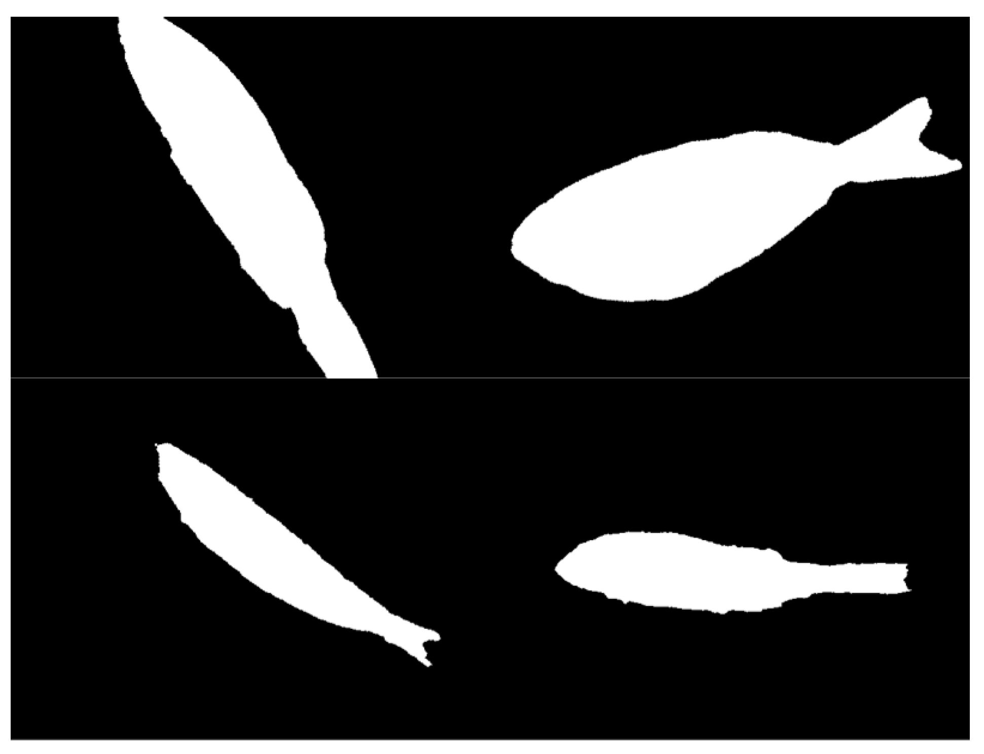
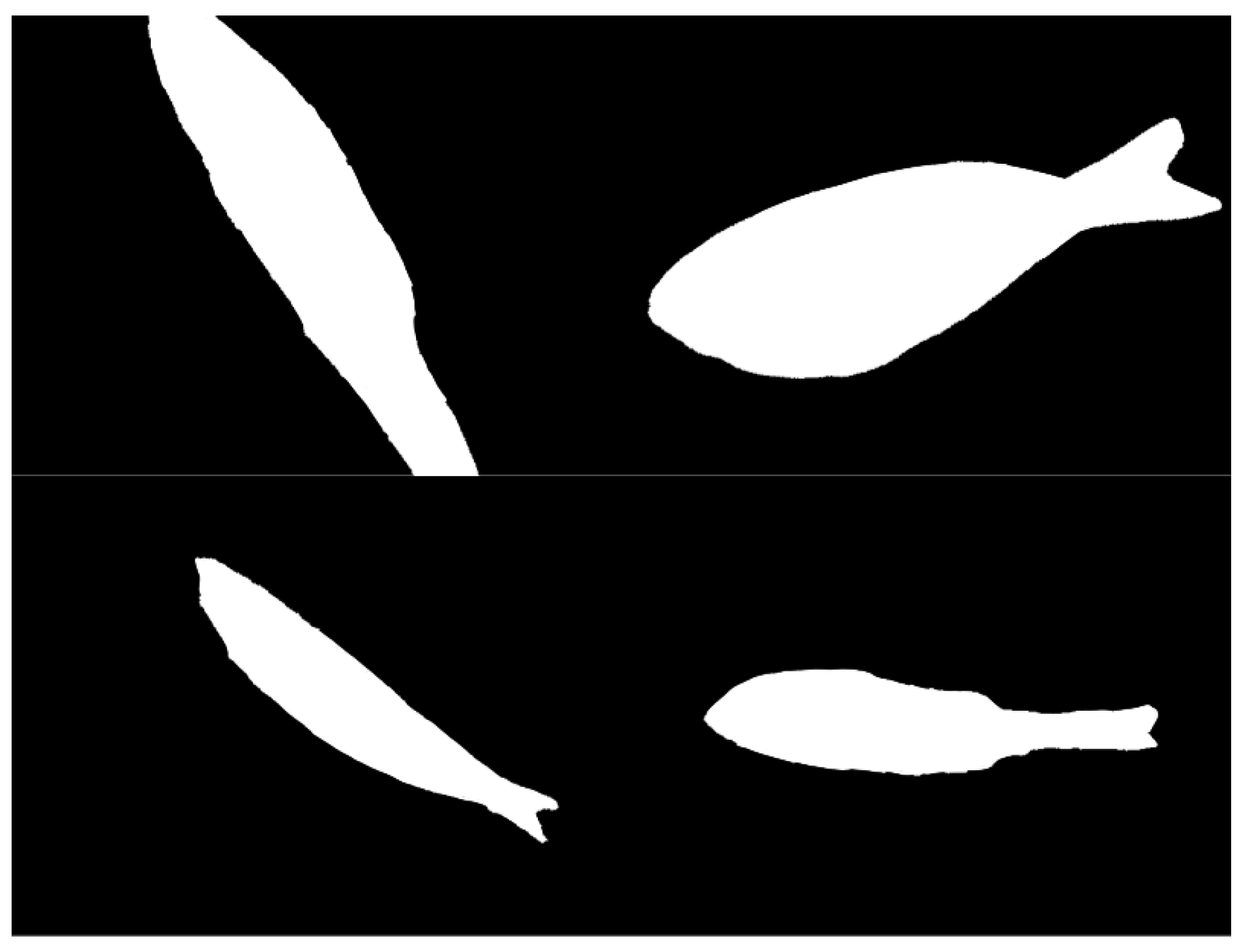
5.2. Segmentation Results

For further comparison, we extracted four images from the fish dataset. These images are pretty distant from each other, which completely reflect the features of this dataset and highlight the difficulties of segmentation. Figure 8, Figure 9, Figure 10, Figure 11, Figure 12, Figure 13, Figure 14, Figure 15 and Figure 16 shows segmentation results. SegNet, FCN16s, and FCN8s lose a significant amount of detail during decoding. Many details are lost during decoding, which makes the segmentation results of these algorithms rough and incorrect at the edges. The segmentation accuracy of U-Net is improved to a certain extent because the hopping connection compensates for some detailed information during the decoding process. Compared with LinkNet, the segmentation results of DenseASPP and FCN32s improve the segmentation results in most regions, except for the regions that are difficult to separate. Our algorithm is quite good at extracting features. It can also overcome indistinguishability between target and background caused by opacity. This is because our model adds a GAN module before the backbone. This pyramid structure allows us to learn the features at the edges better, giving our model a stronger segmentation capability.

6. Discussion

6.1. Ablation Experiment of GAN Module

In order to verify the effectiveness of these GAN modules, the following experiments were conducted.

As observed from

Table 3. Results of different implements of GAN Module.

Method	F1-Score	GA	MIoU	Time (ms)
HRNet + ResNet	0.883	0.891	0.896	18
DeepLab v3 + ResNet	0.922	0.931	0.924	18
DeepLab v3 + Xception	0.873	0.868	0.879	21
no GAN (ours)	0.945	0.940	0.951	27
WGAN	0.961	0.981	0.973	37
BAGAN	0.958	0.973	0.964	32
DCGAN	0.959	0.973	0.961	42

, compared to the models of mainstream backbone, such as ResNet and Xception splicing mainstream segmentation networks, only the MIoU of DeepLab v3 + ResNet combination exceeded 0.9. The model with the GAN module can improve model performance by another 2%. Compared to the comparison model, the maximum improvement is 8% in the MIoU metric. This is mainly due to the fact that deep networks, including backbone and segmentation networks, require a large number of datasets for learning, and the GAN module is suitable for this task.

There is a significant difference in model performance between WGAN, BAGAN, and DCGAN when implementing GAN modules, respectively. Specifically, WGAN performs significantly better than BAGAN and DCGAN, with F1-score, GA, and MIoU reaching 0.961, 0.981, and 0.973, respectively, when implemented with WGAN. In contrast, the model performance of BAGAN and DCGAN decreases significantly. The inference time of DCGAN is the worst among all implementations, reaching 42 ms for a single image. However, the performance of either implementation significantly improved compared to the comparison model without the GAN module. In summary, the GAN module proposed in this paper can indeed improve the segmentation performance of the model.

6.2. Ablation Experiment of Data Enhancement Methods

In order to verify the effectiveness of various data enhancement methods, the following ablation experiments were conducted.

In

Table 4. Results of four enhancement methods.

MixUp	Mosaic	CutOut	CutMix	F1-Score	GA	MIoU	Time (ms)
				0.941	0.936	0.935	36
✓	✓	✓	✓	0.961	0.981	0.973	37
	✓	✓	✓	0.962	0.980	0.973	37
✓		✓	✓	0.961	0.981	0.973	37
✓	✓		✓	0.959	0.970	0.970	37
✓	✓	✓		0.951	0.976	0.966	36

, it can be seen that model performance can be significantly improved by using these four data enhancement methods. However, it seems that from the experimental results these four methods do not contribute equally to the model’s improvement. When the CutOut or CutMix methods are not used, model performance fluctuates significantly, with the F1-score, GA, and MIoU decreasing from 0.961, 0.981, and 0.973 to 0.959, 0.970, 0.970, and 0.951, respectively.

However, when the other two data enhancement methods, MixUp and Mosaic, were not used, there were little significant changes in model performance. The algorithm of MixUp works by overlaying multiple images and generating a synthetic label based on the label of the overlaid image. The algorithm of Mosaic works by cropping multiple images and reorganizing them into a new image. It can be found that both methods work by integrating multiple images at the image scale, and this idea is similar to the manner the GAN module in the network works. The GAN module also generates new images by learning many images of the same label. GAN can also augment the dataset effectively; thus, this paper finally does not use MixUp and Mosaic as data preprocessing methods.

In addition, it can be seen that the use of data augmentation methods have almost no effect on the model inference speed, with only a 1ms change.

6.3. Application on Hbird E203

To deploy the model proposed in this paper into a real-world application scenario, the model is packaged and deployed in conjunction with the Hbrid E203 RISC-V processor. The main reason for choosing this hardware is that it depends on an open-source RISC-V platform and can be highly customized. However, considering its computational power, there is still a need to optimize the computational process of the model in this paper. In this paper, we borrowed Strassen’s [52] optimization idea to optimize matrix multiplication, because the convolutional layer in CNN uses a lot of matrix multiplication operations; thus, optimizing the efficiency of matrix multiplication operations can significantly improve the model’s inference speed. This scheme has the following contributions:

• We encapsulated the model proposed in this paper and saved the parameters of the trained model so that the inference process runs locally.
• We used Strassen’s algorithm to optimize the matrix multiplication method.
• We made developments on the Hbird E203 platform, and model hardware is deployed.

6.4. Limitation

Although our model has achieved the best segmentation results, as shown in Section 5.2, however, there is still room for improvement. As shown in Figure 16, our model can segment the main part of the fish completely, but it still loses a lot of detail at the complicated edges, such as the caudal fin part. This is probably because the proposed method does not optimize the loss function sufficiently for the loss at the edges. Although the robustness of the model can be improved by the GAN module, the current results are still far from the desired results. Addressing these drawbacks is the aimed direction of future work for the authors of this paper.

7. Conclusions

Fish is widely distributed in the world, and fish discrimination and identification are important for improving the efficiency of fisheries sorting as well as for biodiversity studies. Among the methods of fish discrimination and recognition, artificial intelligence depth recognition played an important role in this field. Methods of convolutional neural network design are usually based on UNet and combined with new modules for innovation and improvement. There are some challenges in fish image recognition and segmentation:

• Fish images normally have small pixel areas, have almost the same appearances, and frequently overlap.
• The image recognition process is easily disturbed by the reflection of light and water waves.
• During the image segmentation process, it is easy to ignore the category correlation between adjacent pixel points, resulting in the lack of contextual information.

Therefore, this paper proposes an atrous pyramid GAN segmentation network, aiming to address these above-mentioned problems. The dataset used in this paper contains ten species of fish images, as shown in Figure 2. The contribution of this paper is the following:

• A GAN module is placed in front of the network to address the inadequate training of CNNs due to small datasets and to improve the ability of deep CNNs to extract image features;
• We modified the ASPP algorithm to improve the network’s ability to capture global features;
• Using label smoothing techniques and optimizing the loss function to improve the performance of the segmentation network;
• Matrix multiplication optimization is performed at the instruction level for the Hbrid E203 RISC-V processor to improve the running speed of the model, and the proposed model is packaged and run locally on Hbrid E203.

Although the atrous pyramid GAN segmentation network has surpassed the comparison model, limitations still exist, As mentioned in Section 6.4. It is the future direction of the authors to further improve the segmentation performance of the model at the edges of the fish, such as the caudal fin.

References

1. Marzano, A. Fish and seafood. In The Routledge Handbook of Diet and Nutrition in the Roman World; Routledge: London, UK, 2018; pp. 163–173. [Google Scholar]
2. Halliwell, D.B.; Langdon, R.W.; Daniels, R.A.; Kurtenbach, J.P.; Jacobson, R.A. Classification of freshwater fish species of the northeastern United States for use in the development of indices of biological integrity, with regional applications. In Assessing the Sustainability and Biological Integrity of Water Resources Using Fish Communities; CRC Press: Boca Raton, FL, USA, 2020; pp. 301–337. [Google Scholar]
3. Fautin, D.; Dalton, P.; Incze, L.S.; Leong, J.A.C.; Pautzke, C.; Rosenberg, A.; Sandifer, P.; Sedberry, G.; Tunnell, J.W., Jr.; Abbott, I.; et al. An overview of marine biodiversity in United States waters. PLoS ONE 2010, 5, e11914. [Google Scholar] [CrossRef] [PubMed] [Green Version]
4. Mora, C.; Tittensor, D.P.; Myers, R.A. The completeness of taxonomic inventories for describing the global diversity and distribution of marine fishes. Proc. R. Soc. B Biol. Sci. 2008, 275, 149–155. [Google Scholar] [CrossRef] [PubMed] [Green Version]
5. Cheng, S.; Zhao, K.; Zhang, D. Abnormal Water Quality Monitoring Based on Visual Sensing of Three-Dimensional Motion Behavior of Fish. Symmetry 2019, 11, 1179. [Google Scholar] [CrossRef] [Green Version]
6. Allken, V.; Handegard, N.O.; Rosen, S.; Schreyeck, T.; Mahiout, T.; Malde, K. Fish species identification using a convolutional neural network trained on synthetic data. ICES J. Mar. Sci. 2019, 76, 342–349. [Google Scholar] [CrossRef]
7. Thu, P.T.; Huang, W.C.; Chou, T.K.; Van Quan, N.; Van Chien, P.; Li, F.; Shao, K.T.; Liao, T.Y. DNA barcoding of coastal ray-finned fishes in Vietnam. PLoS ONE 2019, 14, e0222631. [Google Scholar] [CrossRef] [PubMed]
8. Hebert, P.D.; Cywinska, A.; Ball, S.L.; DeWaard, J.R. Biological identifications through DNA barcodes. Proc. R. Soc. Lond. Ser. B Biol. Sci. 2003, 270, 313–321. [Google Scholar] [CrossRef] [PubMed] [Green Version]
9. Ward, R.D.; Hanner, R.; Hebert, P.D. The campaign to DNA barcode all fishes, FISH-BOL. J. Fish Biol. 2009, 74, 329–356. [Google Scholar] [CrossRef] [PubMed]
10. Zhang, J.; Hanner, R. Molecular approach to the identification of fish in the South China Sea. PLoS ONE 2012, 7, e30621. [Google Scholar] [CrossRef]
11. Jin, L.; Yu, J.; Yuan, X.; Du, X. Fish Classification Using DNA Barcode Sequences through Deep Learning Method. Symmetry 2021, 13, 1599. [Google Scholar] [CrossRef]
12. Zhang, Y.; Zhang, Y.; Wa, S.; Liu, Y.; Zhou, X.; Sun, P.; Ma, Q. High-Accuracy Detection of Maize Leaf Diseases CNN Based on Multi-Pathway Activation Function Module. Remote Sens. 2021, 13, 4218. [Google Scholar] [CrossRef]
13. Zhang, Y.; Wang, L.; Chen, A.; Zhang, Y.; Wang, X.; Zhang, Y.; Shen, Q.; Xue, Y. AK-DL: A Shallow Neural Network Model for Diagnosing Actinic Keratosis with Better Performance than Deep Neural Networks. Diagnostics 2020, 10, 217. [Google Scholar] [CrossRef]
14. Zhang, Y.; Zhang, Y.; Liu, X.; Wa, S.; Liu, Y.; Kang, J.; Lv, C. GenU-Net++: An Automatic Intracranial Brain Tumors Segmentation Algorithm on 3D Image Series with High Performance. Symmetry 2021, 13, 2395. [Google Scholar] [CrossRef]
15. Zhang, Y.; Zhang, Y.; He, S.; Wa, S.; Zong, Z.; Liu, Y. Using Generative Module and Pruning Inference for the Fast and Accurate Detection of Apple Flower in Natural Environments. Information 2021, 12, 495. [Google Scholar] [CrossRef]
16. Zhang, Y.; Zhang, Y.; Wa, S.; Sun, P.; Wang, Y. Pear Defect Detection Method Based on ResNet and DCGAN. Information 2021, 12, 397. [Google Scholar] [CrossRef]
17. Cao, F.; Zhao, H. Automatic Lung Segmentation Algorithm on Chest X-ray Images Based on Fusion Variational Auto-Encoder and Three-Terminal Attention Mechanism. Symmetry 2021, 13, 814. [Google Scholar] [CrossRef]
18. Konovalov, D.A.; Saleh, A.; Bradley, M.; Sankupellay, M.; Marini, S.; Sheaves, M. Underwater fish detection with weak multi-domain supervision. In Proceedings of the 2019 International Joint Conference on Neural Networks (IJCNN), Budapest, Hungary, 14–19 July 2019; pp. 1–8. [Google Scholar]
19. Lee, Y.H.; Kim, H.J. Implementation of Fish Detection Based on Convolutional Neural Networks. J. Semicond. Disp. Technol. 2020, 19, 124–129. [Google Scholar]
20. Štefanič, P.; Cigale, M.; Jones, A.C.; Knight, L.; Taylor, I.; Istrate, C.; Suciu, G.; Ulisses, A.; Stankovski, V.; Taherizadeh, S.; et al. SWITCH workbench: A novel approach for the development and deployment of time-critical microservice-based cloud-native applications. Future Gener. Comput. Syst. 2019, 99, 197–212. [Google Scholar] [CrossRef]
21. Cui, S.; Zhou, Y.; Wang, Y.; Zhai, L. Fish detection using deep learning. Appl. Comput. Intell. Soft Comput. 2020, 2020, 3738108. [Google Scholar] [CrossRef]
22. Schwartz, S.T. Automated High-Throughput Organismal Image Segmentation Using Deep Learning for Massive Phenotypic Analysis; University of California: Los Angeles, CA, USA, 2021. [Google Scholar]
23. Majumder, A.; Rajbongshi, A.; Rahman, M.M.; Biswas, A. Local freshwater fish recognition using different cnn architectures with transfer learning. Int. J. Adv. Sci. Eng. Inf. Technol. 2021, 11, 1078–1083. [Google Scholar] [CrossRef]
24. Ronneberger, O.; Fischer, P.; Brox, T. U-net: Convolutional networks for biomedical image segmentation. In International Conference on Medical Image Computing and Computer-Assisted Intervention; Springer: Berlin/Heidelberg, Germany, 2015; pp. 234–241. [Google Scholar]
25. Zhou, Z.; Siddiquee, M.M.R.; Tajbakhsh, N.; Liang, J. Unet++: A nested u-net architecture for medical image segmentation. In Deep Learning in Medical Image Analysis and Multimodal Learning for Clinical Decision Support; Springer: Berlin/Heidelberg, Germany, 2018; pp. 3–11. [Google Scholar]
26. Yu, C.; Liu, Y.; Hu, Z.; Xia, X. Precise segmentation and measurement of inclined fish’s features based on U-net and fish morphological characteristics. Appl. Eng. Agric. 2021, 38, 37–48. [Google Scholar]
27. Labao, A.B.; Naval, P.C., Jr. Cascaded deep network systems with linked ensemble components for underwater fish detection in the wild. Ecol. Inform. 2019, 52, 103–121. [Google Scholar] [CrossRef]
28. Miyazono, T.; Saitoh, T. Fish species recognition based on CNN using annotated image. In IT Convergence and Security 2017; Springer: Berlin/Heidelberg, Germany, 2018; pp. 156–163. [Google Scholar]
29. Ibrahim, A.; Ahmed, A.; Hussein, S.; Hassanien, A.E. Fish image segmentation using salp swarm algorithm. In International Conference on Advanced Machine Learning Technologies and Applications; Springer: Berlin/Heidelberg, Germany, 2018; pp. 42–51. [Google Scholar]
30. Wang, S.H.; Zhao, J.W.; Chen, Y.Q. Robust tracking of fish schools using CNN for head identification. Multimed. Tools Appl. 2017, 76, 23679–23697. [Google Scholar] [CrossRef]
31. Chen, L.C.; Papandreou, G.; Kokkinos, I.; Murphy, K.; Yuille, A.L. Deeplab: Semantic image segmentation with deep convolutional nets, atrous convolution, and fully connected crfs. IEEE Trans. Pattern Anal. Mach. Intell. 2017, 40, 834–848. [Google Scholar] [CrossRef] [Green Version]
32. Thampi, L.; Thomas, R.; Kamal, S.; Balakrishnan, A.A.; Haridas, T.M.; Supriya, M. Analysis of U-Net Based Image Segmentation Model on Underwater Images of Different Species of Fishes. In Proceedings of the 2021 International Symposium on Ocean Technology (SYMPOL), Kochi, India, 9–11 December 2021; pp. 1–5. [Google Scholar]
33. Krizhevsky, A.; Sutskever, I.; Hinton, G. ImageNet Classification with Deep Convolutional Neural Networks. In Advances in Neural Information Processing Systems, Proceedings of the Neural Information Processing Systems Conference (NIPS 2012), Lake Tahoe, NV, USA, 3–6 December 2012; Curran Associates, Inc.: Sussex, NB, Canada, 2012; Volume 25, Available online: https://proceedings.neurips.cc/paper/2012/file/c399862d3b9d6b76c8436e924a68c45b-Paper.pdf (accessed on 12 December 2021).
34. Wang, W.; Zhou, T.; Yu, F.; Dai, J.; Konukoglu, E.; Van Gool, L. Exploring cross-image pixel contrast for semantic segmentation. In Proceedings of the IEEE/CVF International Conference on Computer Vision, Montreal, BC, Canada, 11–17 October 2021; pp. 7303–7313. [Google Scholar]
35. Zhou, T.; Li, L.; Li, X.; Feng, C.M.; Li, J.; Shao, L. Group-Wise Learning for Weakly Supervised Semantic Segmentation. IEEE Trans. Image Process. 2021, 31, 799–811. [Google Scholar] [CrossRef] [PubMed]
36. Zhou, T.; Li, J.; Wang, S.; Tao, R.; Shen, J. Matnet: Motion-attentive transition network for zero-shot video object segmentation. IEEE Trans. Image Process. 2020, 29, 8326–8338. [Google Scholar] [CrossRef] [PubMed]
37. Long, J.; Shelhamer, E.; Darrell, T. Fully convolutional networks for semantic segmentation. In Proceedings of the IEEE Conference on Computer Vision and Pattern Recognition, Boston, MA, USA, 7–12 June 2015; pp. 3431–3440. [Google Scholar]
38. Ulucan, O.; Karakaya, D.; Turkan, M. A Large-Scale Dataset for Fish Segmentation and Classification. In Proceedings of the 2020 Innovations in Intelligent Systems and Applications Conference (ASYU), Istanbul, Turkey, 15–17 October 2020; pp. 1–5. [Google Scholar]
39. Zhang, H.; Cisse, M.; Dauphin, Y.N.; Lopez-Paz, D. mixup: Beyond empirical risk minimization. arXiv 2017, arXiv:1710.09412. [Google Scholar]
40. Bochkovskiy, A.; Wang, C.Y.; Liao, H.Y.M. Yolov4: Optimal speed and accuracy of object detection. arXiv 2020, arXiv:2004.10934. [Google Scholar]
41. DeVries, T.; Taylor, G.W. Improved regularization of convolutional neural networks with cutout. arXiv 2017, arXiv:1708.04552. [Google Scholar]
42. Yun, S.; Han, D.; Oh, S.J.; Chun, S.; Choe, J.; Yoo, Y. Cutmix: Regularization strategy to train strong classifiers with localizable features. In Proceedings of the IEEE/CVF International Conference on Computer Vision, Seoul, Korea, 27 October–2 November 2019; pp. 6023–6032. [Google Scholar]
43. Chen, S.; Haralick, R.M. Recursive erosion, dilation, opening, and closing transforms. IEEE Trans. Image Process. 1995, 4, 335–345. [Google Scholar] [CrossRef]
44. Arjovsky, M.; Bottou, L. Towards principled methods for training generative adversarial networks. arXiv 2017, arXiv:1701.04862. [Google Scholar]
45. Arjovsky, M.; Chintala, S.; Bottou, L. Wasserstein generative adversarial networks. In Proceedings of the International Conference on Machine Learning, Sydney, Australia, 6–11 August 2017; pp. 214–223. Available online: https://proceedings.mlr.press/v70/arjovsky17a.html (accessed on 12 December 2021).
46. Mariani, G.; Scheidegger, F.; Istrate, R.; Bekas, C.; Malossi, C. Bagan: Data augmentation with balancing gan. arXiv 2018, arXiv:1803.09655. [Google Scholar]
47. Odena, A.; Olah, C.; Shlens, J. Conditional image synthesis with auxiliary classifier gans. In Proceedings of the International Conference on Machine Learning, Sydney, Australia, 6–11 August 2017; pp. 2642–2651. Available online: https://proceedings.mlr.press/v70/odena17a.html (accessed on 12 December 2021).
48. He, K.; Zhang, X.; Ren, S.; Sun, J. Deep Residual Learning for Image Recognition. In Proceedings of the 2016 IEEE Conference on Computer Vision and Pattern Recognition (CVPR), Las Vegas, NV, USA, 27–30 June 2016. [Google Scholar]
49. Yang, M.; Yu, K.; Zhang, C.; Li, Z.; Yang, K. Denseaspp for semantic segmentation in street scenes. In Proceedings of the IEEE Conference on Computer Vision and Pattern Recognition, Salt Lake City, UT, USA, 18–23 June 2018; pp. 3684–3692. [Google Scholar]
50. Badrinarayanan, V.; Kendall, A.; Cipolla, R. Segnet: A deep convolutional encoder-decoder architecture for image segmentation. IEEE Trans. Pattern Anal. Mach. Intell. 2017, 39, 2481–2495. [Google Scholar] [CrossRef] [PubMed]
51. Woo, S.; Kim, D.; Cho, D.; Kweon, I.S. Linknet: Relational embedding for scene graph. arXiv 2018, arXiv:1811.06410. [Google Scholar]
52. Strassen, V. Gaussian elimination is not optimal. Numer. Math. 1969, 13, 354–356. [Google Scholar] [CrossRef]
Figure 1. Illustration of spatial pyramid pooling layer.
Electronics 11 00911 g001
Figure 2. Dataset visualization. (AI) shows multiple targets and multiple scales of the dataset: (A) is Black Sea Sprat; (B) is Gilt-Head Bream; (C) is Hourse Mackerel; (D) is Red Mullet; (E) is Red Sea Bream; (F) is Sea Bass; (G) is Shrimp; (H) is Striped Red Mullet; (I) is Trout.
Electronics 11 00911 g002
Figure 3. Illustration of enhancement methods. (A) Mixup; (B) Mosaic; (C) Cutout; (D) CutMix.
Electronics 11 00911 g003
Figure 4. Processing of removal of useless details.
Electronics 11 00911 g004
Figure 5. Structure of the atrous pyramid GAN segmentation network.
Electronics 11 00911 g005
Figure 6. Network structure of BAGAN.
Electronics 11 00911 g006
Figure 7. Warmup learning rate schedule.
Electronics 11 00911 g007
Figure 8. The ground truth of the dataset.
Electronics 11 00911 g008
Figure 9. The segmentation results of FCN8s.
Electronics 11 00911 g009
Figure 10. The segmentation results of FCN16s.
Electronics 11 00911 g010
Figure 11. The segmentation results of FCN32s.
Electronics 11 00911 g011
Figure 12. The segmentation results of DenseASPP.
Electronics 11 00911 g012
Figure 13. The segmentation results of SegNet.
Electronics 11 00911 g013
Figure 14. The segmentation results of LinkNet.
Electronics 11 00911 g014
Figure 15. The segmentation results of UNet.
Electronics 11 00911 g015
Figure 16. The segmentation results of our model.
Electronics 11 00911 g016