Investigations on Field Distribution along the Earth’s Surface of a Submerged Line Current Source Working at Extremely Low Frequency Band

Abstract

A numerical analysis on field distribution along the Earth’s surface of a line current source submerged in the ground is conducted in this paper to investigate the potential of the extremely low frequency (ELF) technology in the envisioned long-distance communication techniques. The problem is modeled as a submerged horizontal electric dipole (HED) in a two-layered homogeneous half space and solved by the combined numerical methods of the Romberg-Euler method and Gauss-Laguerre method. The model is validated by experimental results with only a maximum 10% error at 9 Hz around 490 m. Meanwhile, the study shows that the ELF signals emitted by a submerged line current source can transmit at least 1 km with a current sensor sensitivity of 0.1 pT. These results indicate the possibility of applying of ELF technology to long-distance communication or the long-distance transmedia detection.

1. Introduction

The investigation on extremely low frequency electromagnetic wave distribution has been a classical problem because of the wide applications of technologies in marine engineering such as undersea detection, undersea sensor networks, coastal surveillance, seabed communication, etc. The problem has attracted increasing attention and investigations, which are mainly focused on field distribution in stratified media since the first analysis for the electromagnetic wave along the planar boundary as early as 1907 [1]. Then, Dr. Sommerfeld investigated the excited field of a dipole in the multilayered lossy media where the concept of Sommerfeld integrals [2] is proposed, and a field theory in a homogeneous half-space is fully developed in [3]. Since the attenuation rates of ELF waves could be as low as 1 dB/1000 km, stated in reference [4], the potential of the applications of such technologies to long-distant communication has gained researcher’s attention. Currently, numerous investigations have been conducted on the ELF EM wave propagation based on an isotropic conductivity Earth model where field distribution by a dipole submerged in a lossy media is thoroughly studied [5,6,7,8,9]. Chave, A.D. studies undersea communication by free propagation of ULF/ELF electromagnetic waves from harmonic dipole sources located on or near the sea floor [10]. In 2017, the scenario of a three-layered conducting media including air, seawater and seabed has been discussed [11], where the ELF electromagnetic fields generated by a submerged horizontal electric dipole in the shallow sea are fully investigated. Later, the studies have been extended to the detection of underwater moving objects [12,13]. In 2018, the seabed environment is treated as a three-layered media and the field distribution is numerically investigated [14]. At the same time, the ELF EM signal has widely used in drilling system to carry downhole measurement data where the studies of channel models and demodulation techniques are essential [15]. Meanwhile, the existence of Zenneck surface wave has drawn researchers’ attention, which was proposed by Baño [3]. Successive studies have been conducted by Dr. King on lateral electromagnetic waves in 1980s while the work is extended from two-layered to three-layered media by Dr. Dunn [16,17,18,19].

It can be easily observed that large amounts of studies have been conducted on theoretical analysis and numerical modeling, but there is scarcity of fulfillment of the transmission of ELF signals [20,21,22]. Furthermore, the majority of current measurements are limited to the propagation of ELF wave in the sea while the work on wave propagation along Earth’s surfaces remains vacant. To fill these gaps, an experiment is first designed with a line current source submerged in the ground where the emitted magnetic field signals along the mountain surface are collected by the commercial magnetic sensor. Then, the submerged line current source is modeled as a submerged horizontal electric dipole, and the field distribution is calculated by a combined method of Romberg-Euler method and Gauss-Laguerre method. Furthermore, numerical results are compared with experimental ones to validate the models and investigate field performances.

The remainder of the paper is organized as follows. Section 2 discusses the theoretical model of the line current source while the experiment’s descriptions are illustrated in Section 3. At the same time, the performance of the numerical model is also investigated in Section 3. In the end, a brief conclusion is drawn in Section 4.

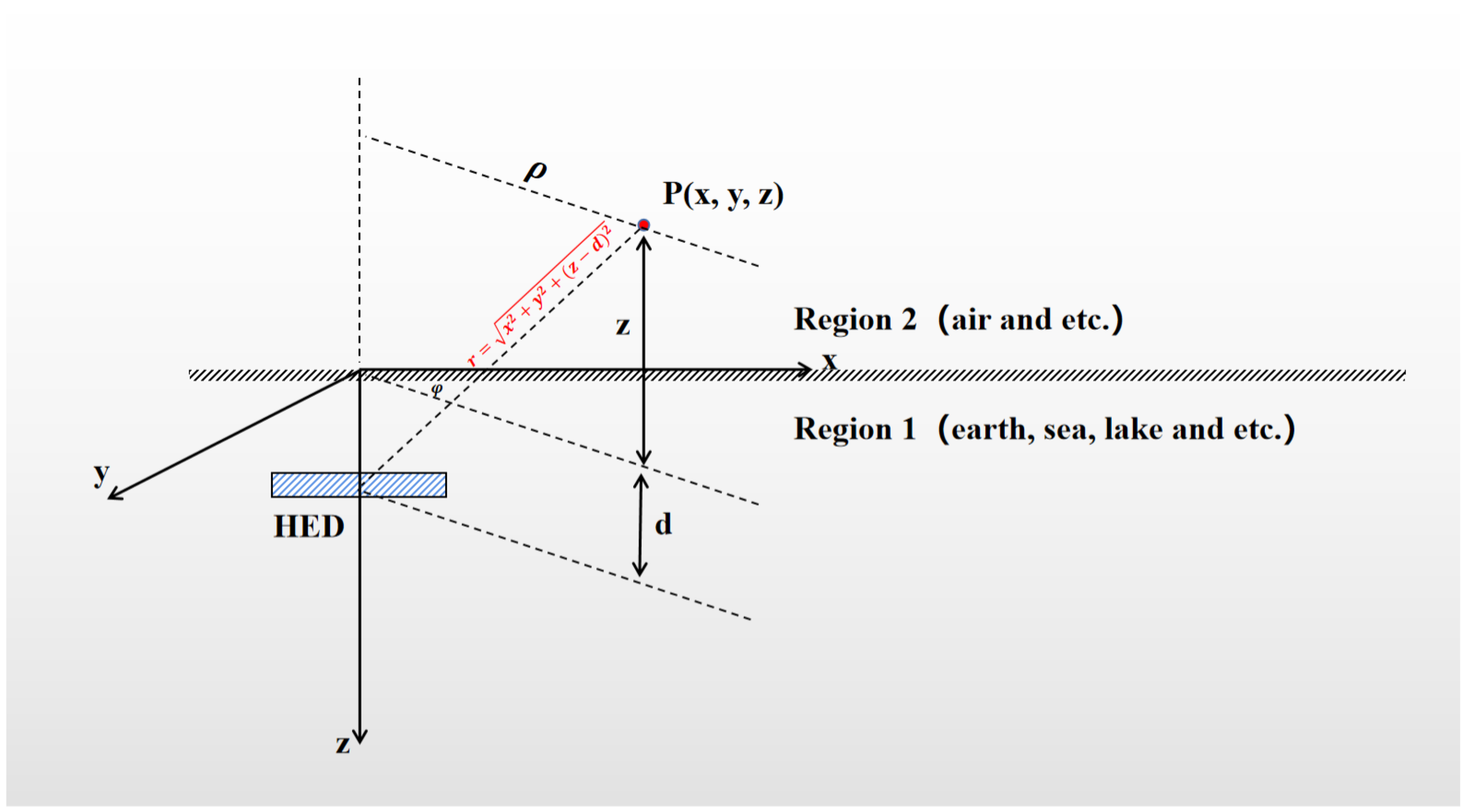
2. Theoretical Model

To save the space and to enhance performance, a horizontal line current is adopted in our study, which is approximated as a horizontal electric dipole source theoretically. Not losing generality, an x-directed horizontal electric dipole is investigated, as shown in Figure 1, which is placed at point $z=d$ on the downward-directed z-axis in the half-space where $z\ge 0$, which is region 1. Region 2 is the space where $z\le 0$. The wave number of each region is $k_j=\omega \sqrt{{\mu }_j{ϵ}_j}$, where ${ϵ}_j={ϵ}_0({ϵ}_{rj}-j{\sigma }_i/\omega {ϵ}_0)$, ${\mu }_j={\mu }_{ri}{\mu }_0$ and $j=1,2$. ${ϵ}_0$ and ${\mu }_0$ are the permittivity and permeability of free space. Since soil and rock are all non-magnetic, ${\mu }_{r1}={\mu }_{r2}=1$.

Therefore, the problem can be described as follows. Maxwell’s equation in the two region are as follows:

$$\begin{array}{cc}\hfill \nabla \times {\mathbf{E}}_j& =i\omega {\mathbf{B}}_j\hfill \\ \hfill \nabla \times {\mathbf{B}}_j& ={\mu }_0(-i\omega {ϵ}_j{\mathbf{E}}_j+\mathbf{J})\hfill \end{array}$$

(1)

where $\mathbf{J}=\widehat{\mathbf{x}}Il\delta \left(x\right)\delta \left(y\right)\delta (z-d)$ is the electric moment.

${\mathbf{E}}_j$ and ${\mathbf{B}}_j$ will be solved with the following boundary conditions.

$$\begin{array}{cc}\hfill E_{1x}(x,y,0)& =E_{2x}(x,y,0);\hfill \\ \hfill E_{1y}(x,y,0)& =E_{2y}(x,y,0);\hfill \\ \hfill k_1^2{E}_{1z}(x,y,0)& =k_2^2{E}_{2z}(x,y,0);\hfill \\ \hfill {\mathbf{B}}_1(x,y,0)& ={\mathbf{B}}_2(x,y,0)\hfill \end{array}$$

(2)

To investigate the performance of the wave, we usually measure the fields in region 2. Thus, the field components in it are solved and illustrated below [23]:

$$\begin{array}{cc}\hfill E_{2\rho }& =-\frac{Il\omega {\mu }_0}{4\pi }cos\varphi {\int }_0^{\infty }(\frac{[J_0\left(\lambda \rho \right)+J_2\left(\lambda \rho \right)]}{M}+\frac{{\gamma }_1{\gamma }_2[J_0\left(\lambda \rho \right)-J_2\left(\lambda \rho \right)]}{N})e^{i({\gamma }_{1}d-{\gamma }_{2}z)}\lambda d\lambda \hfill \\ \hfill E_{2\varphi }& =\frac{Il\omega {\mu }_0}{4\pi }sin\varphi {\int }_0^{\infty }(\frac{[J_0\left(\lambda \rho \right)-J_2\left(\lambda \rho \right)]}{M}+\frac{{\gamma }_1{\gamma }_2[J_0\left(\lambda \rho \right)+J_2\left(\lambda \rho \right)]}{N})e^{i({\gamma }_{1}d-{\gamma }_{2}z)}\lambda d\lambda \hfill \\ \hfill E_{2z}& =-\frac{Il\omega {\mu }_0}{2\pi }cos\varphi {\int }_0^{\infty }\frac{{\gamma }_1{J}_1\left(\lambda \rho \right)e^{i({\gamma }_{1}d-{\gamma }_{2}z){\lambda }^2}}{N}d\lambda \hfill \\ \hfill B_{2\rho }& =\frac{Il{\mu }_0}{4\pi }sin\varphi {\int }_0^{\infty }(\frac{{\gamma }_2[J_0\left(\lambda \rho \right)-J_2\left(\lambda \rho \right)]}{M}+\frac{k_2^2{\gamma }_1[J_0\left(\lambda \rho \right)+J_2\left(\lambda \rho \right)]}{N})e^{i({\gamma }_{1}d-{\gamma }_{2}z)}\lambda d\lambda \hfill \\ \hfill B_{2\varphi }& =\frac{Il{\mu }_0}{4\pi }cos\varphi {\int }_0^{\infty }(\frac{{\gamma }_2[J_0\left(\lambda \rho \right)+J_2\left(\lambda \rho \right)]}{M}+\frac{k_2^2{\gamma }_1[J_0\left(\lambda \rho \right)-J_2\left(\lambda \rho \right)]}{N})e^{i({\gamma }_{1}d-{\gamma }_{2}z)}\lambda d\lambda \hfill \\ \hfill B_{2z}& =\frac{iIl{\mu }_0}{2\pi }sin\varphi {\int }_0^{\infty }\frac{J_1\left(\lambda \rho \right)e^{i({\gamma }_{1}d-{\gamma }_{2}z){\lambda }^2}}{M}d\lambda \hfill \end{array}$$

(3)

where $M\equiv {\gamma }_1+{\gamma }_2$, $N\equiv k_1^2{\gamma }_2+k_2^2{\gamma }_1$ and $J_n$ is the Bessel function. ${\gamma }_j^2=k_j^2-{\xi }^2-{\eta }^2$, which is defined by the translational invariance $\mathbf{E}(x,y,z)=\frac{1}{{\left(2\pi \right)}^2}{\int }_{-\infty }^{\infty }d\xi {\int }_{-\infty }^{\infty }d\eta e\mathbf{E}(\xi ,\eta ,z)$ [23].

The calculation of Equation (3) would require the analysis of the Sommerfeld Integral, for which its general form is described as follows:

$$S={\int }_0^{\infty }f\left(\lambda \right)J_n\left(\lambda \rho \right)e^{-g\left(\lambda \right)}d\lambda$$

(4)

where $f\left(\lambda \right)$ and $g\left(\lambda \right)$ are the complex function of the frequency and medium properties. $J_n\left(\lambda \rho \right)$ is the first kind Bessel function of order n. To evaluate SI, numerous poles would appear in the integral path, which would make the numerical calculation divergent. To solve such problems, numerous techniques have been developed and a combined numerical method with the Gauss-Laguerre method and Romberg–Euler method is applied in the paper based on the current studies [24]. A brief introduction of both methods is illustrated as follows.

2.1. Gauss-Laguerre Method

The Gauss-Laguerre quadrature method can be expressed as follows:

$${\int }_0^{\infty }f\left(x\right)e^{-x}dx\approx \sum _{i=0}^n{A}_{i}f\left(x_i\right)$$

(5)

where $x_i$ is the ith null point of the Laguerre polynomial of order $N+1$, and $w_i$ is the corresponding weight; they can be easily obtained from the relevant literature. The approximation in Equation (5) is exact when $f\left(x\right)$ is a polynomial of a degree less than $2N+1$; thus, the Guass–Laguerre quadrature succeeds if $f\left(x\right)$ can be adequately represented by a polynomial of finite order for range $[0,\infty ]$. It is obvious that the higher order Laguerre polynomial can produce more accurate integral results but involves more computation time. For example, in Equation (3), by permitting the following, $B_{2z}$ can be evaluated by Equation (5).

$$f\left(x\right)=\frac{J_1\left(x\rho \right)e^{i({\gamma }_{1}d-{\gamma }_{2}z)x^2}{e}^x}{M}$$

(6)

Although more complicated than $B_{2z}$, the other components can also be evaluated in this manner.

This method is suitable for the case where the horizontal distance is less than the vertical distance, i.e., $\rho \le z$.

2.2. Romberg-Euler Method

The Romberg–Euler composite method can by expressed as follows:

$$S={\int }_0^{\infty }W\left(\lambda \right)J_n\left(\lambda \rho \right)e^{-g\left(\lambda \right)}d\lambda \approx \sum _{m=1}^{\infty }{\int }_{x_{m-1}}^{x_m}W\left(\lambda \right)J_n\left(\lambda \rho \right)e^{-g\left(\lambda \right)}d\lambda =\sum _{m=1}^{\infty }{B}_m=S_p$$

(7)

where $x_0=0$, and $x_m$ is the first root of the Bessel function $J_n\left(\lambda \rho \right)$. The value of the integral S is the limit to which sequence $S_p$ converges.

The termination condition of the iteration is stated as follows.

$$|\frac{\Delta S_p}{S_p}|=|\frac{(S_p-S_{p-1})}{S_p}|=|\frac{B_p}{S_p}|<ϵ$$

(8)

Take $B_z$ in Equation (3) as an example again; here, we can permit $W\left(\lambda \right)=\frac{1}{M}$ and $g\left(\lambda \right)=-i({\gamma }_{1}d-{\gamma }_{2}z){\lambda }^2$. Then, $B_{2z}$ can be evaluated by Equation (7).

The integration is performed between the zeros of the Bessel function, and the truncated infinite integral is expressed as a sum of integral between successive Bessel zeros. Since the envelope of $W\left(\lambda \right)$ decays more slowly than the rapidly oscillating Bessel function, especially for large values of the argument, the Euler transform can be used to speed up the converge of the piecewise integration sequence. The Romberg quadrature method is adopted for piecewise integration in $B_m$.

To evaluate the performance of the above methods, the calculation times are usually compared with different values of $\frac{\rho }{z}$. Studies shows that when $\rho >z$, the Romberg–Euler method outperforms the Gauss-Laguerre one [24] and when $\rho <z$, Gauss-Laguerre method performs better.

3. Experiments and Results Discussions

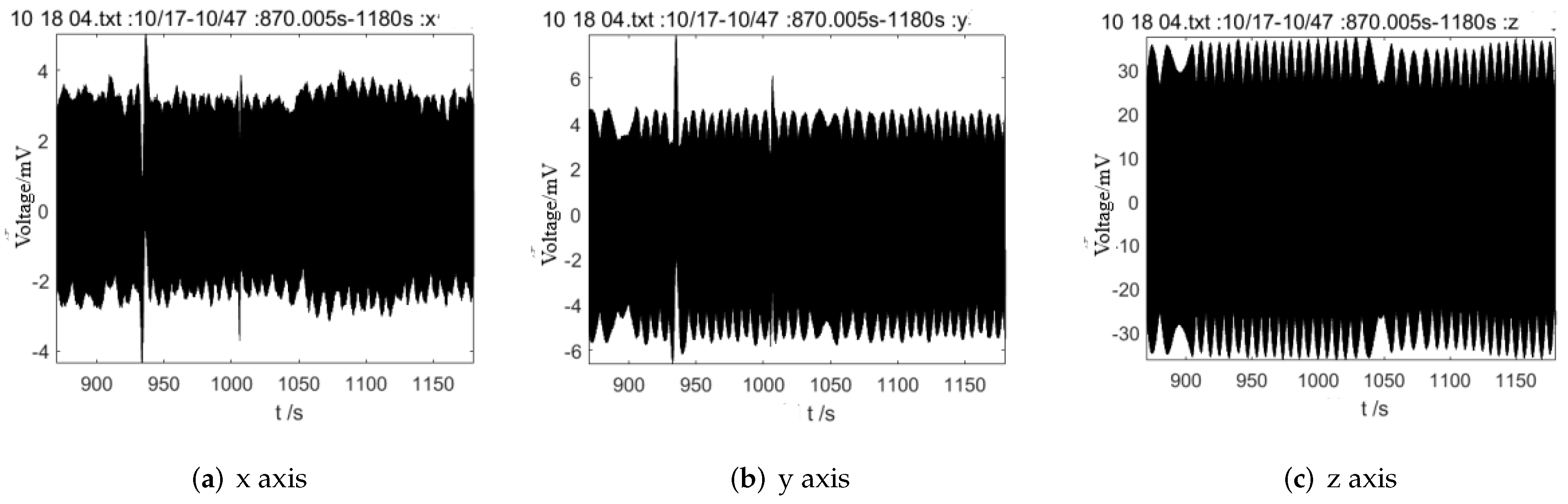
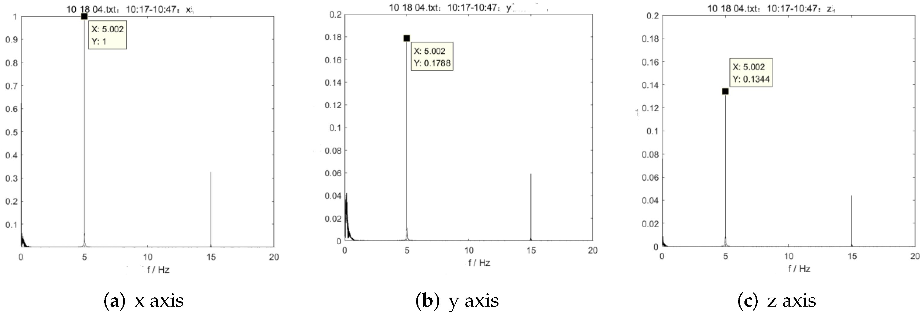
3.1. Experiments Description

An experiment has been conducted in a reservoir in the Qin Mountain in Northwestern China (109°49′ E, 33°42′ N), shown in Figure 2a, to study the radiation performances of the submerged line current and the wave diffusion along the Earth’s surface. The soil of the region was composed of mud, sand and crushed granite where conductivity is around 5 S/m. The line current source is buried around 1-m deep in a shallow horizontal layer and connected to a transmitter which would send ELF signals. The schematics of the source are shown in Figure 2b. In the experiment, the copper wire is around 200 m long, the radius is around 1 mm and the emission current is constantly 0.07 A. Thus, the emission intensity of the envisioned electric dipole is 14 Am. The emitting frequencies of the ELF signals are set at 3 Hz, 5 Hz and 9 Hz.

A commercial magnetic sensor produced by Huashun Ltd. (Xi’an, China) with a high sensitivity of 216 mV/nT and low noise level of 0.057 pT/$\sqrt{\mathrm{Hz}}$ at 1 Hz, shown in Figure 3a, is adopted to collect magnetic signals. The details of the ferrite rod sensor is shown in

Table 1. Parameters of the ferrite rod sensor.

Paramters	Values
Bandwith	0.1 Hz–200 Hz
Noise Level	0.057 pT/$\sqrt{\mathrm{Hz}}$@1 Hz
Measurement Range	±10 nT
Output Voltage	±10 V
NRP	≤0.35 W

. To investigate the magnetic fields’ complete performance, three sensors were perpendicularly assembled relative each other, shown in Figure 3b, which are placed as high as 20 cm away from the Earth’s surface. The three-axis magnetic collection system would transfer the collecting magnetic field into voltage with 24-bit sampling, which would be recorded in the data acquisition system based on NI modules with sampling rates of 200 Hz, as shown in Figure 3c. To obtain the field strength, the values at the frequency of interest would be collected and transferred by sensitivity. A 5 Hz square-wave signal collected by the system is shown in Figure 4 and Figure 5.

To check the source states, a reference point is fixed closely to the line current source, which records the received magnetic signal at 50 m. Other spots at 490 m, 632 m and 735 m away from the source are chosen according to the environment in the mountain. Figure 3c shows the receiver placed in a 5-m deep cave at an distance of 490 m.

3.2. Results Discussion

3.2.1. Validation of the Numerical Model

To investigate the performance of the proposed numerical model and the combined method, the measured magnetic fields strengths are compared with the numerical results of the submerged HED model. As shown in Figure 1, the source is selected as an HED with the electric moment of 14 Am, and it was located in a two-half homogeneous space. The HED is 1 m away from the interface and located in region 1 where ${ϵ}_r=10,{\mu }_r=1,\sigma =5$ S/m, which are the general parameters of the soil. Region 2 would be air with ${ϵ}_r=1,{\mu }_r=1,\sigma =0$ S/m, and the fields of interest are analyzed.

The comparison of the two field strengths is illustrated in Figure 6 with distance as the horizontal axis. From the figure, we can see that both data agree well but with some slight differences with 0.026 nT as the maximum (10%) at 9 Hz around 490 m. The errors are mainly caused by the ideal assumption of the ideal layered structures and the noise produced by the collection system and introduced by the environment. Thus, it can be easily concluded that the proposed model would be a promising substitute for the preliminary study of such channels at the ELF band, especially for locations that are hard to reach. At the same time, it can be easily observed that, in the ELF band, the influences of the frequency on field strength are limited, especially in the closer range.

3.2.2. Investigations on the Field Distribution

From the previous study, it can be clearly concluded that a magnetic ELF signals could be produced by a submerged line current and such signals can travel along the Earth’s surface. Although the signal strengths are at the level of $nT$, magnetic signals can be collected at least 1 km for all ELF bands up to 9 Hz due to the development of the current sensor technology, which would increase sensitivity to the level of $sub$-$pT$.

The electric field and magnetic field distributions at $xoy$-$plane$ ($z=1$ m) of the ELF wave at 5 Hz with an x-axis located HED as the source are shown in Figure 7. The electric moments is 14 Am, and the figure is illustrated in logarithm form. A typical distribution of an electric dipole can be observed and the magnetic field suffers less power loss than the electric field, which indicates the potential of the magnetic signals of ELF communication techniques.

The power loss of the signals is illustrated in Figure 8. To calculate path loss, the magnitude of the magnetic field was measured and recorded at 50 m, which was chosen as reference $B_o$. Then, the ratio of the field magnitude at ith point $B_i$ to the ones at reference point $B_o$ would be calculated and followed by a logarithmic operation, i.e., $PL=20lg\frac{B_i}{B_o}$. From the figure, it can be observed that path loss increases with an increase in the distance, but frequency would have limited impact.

Additionally, a modified Friis Model [25] is applied to model path loss:

$$PL=alg\frac{d}{d_0}+b\frac{d}{d_0}+c$$

(9)

where $d_0$ is 50 m, a is the spreading path loss index and b refers to the absorption index.

The corresponding parameters are shown in

Table 2. Parameters of modified path-loss models.

Freq.	a	b	c	SSE	RMSE
3 Hz	30.86	−0.87	0.46	4.43	0.22
5 Hz	39.56	−0.85	2.11	25.99	0.53
9 Hz	46.17	−0.63	3.43	4.83	0.23

. From the table, it can be easily observed that the spreading path loss index a and absorption index b would be at the same order for different frequencies, as indicated by the figure. The spreading path loss index is around 40, which indicates the appearance of other types of wave transmission in addition to traditional direct propagation, while the absorption index is close to zero because of the non-lossy properties of mountain rocks, which would render absorption loss negligible.

4. Conclusions

In the paper, the emission fields of a submerged line current source in the ground are theoretically and experimentally analyzed. The results showed that the submerged line current source can emit ELF signals and can be modeled as a submerged HED, which would simplify the process for the communication system’s design. In addition, the initial studies of the path loss models indicate the potential of the ELF techniques for super long-distance communication, which would pave the way for future studies. However, to render wide ELF bands available and usable, the antenna and transceiver techniques should be fully developed, and they are still in their early phases; thus, more research work should be conducted. As an initial study on such techniques, much work still needs to be performed, such as more experiments and complete theoretical analyses to enrich the database and to explain the peculiarities in detail.

References

1. Zenneck, J. Propagation of plane electromagnetic waves along a plane conducting surface and its bearing on the theory of transmission in wireless telegraphy. Ann. Phys. 1907, 23, 846–866. [Google Scholar] [CrossRef] [Green Version]
2. Sommerfeld, A. Propagation of waves in wireless telegraphy. Ann. Phys. 1909, 333, 665–736. [Google Scholar] [CrossRef] [Green Version]
3. Baños, A.J. Dipole Radiation in the Presence of a Conducting Half-Space; Pergamon Press: Oxford, UK, 1966. [Google Scholar]
4. Pappert, R.A.; Moler, W.F. Propagation theory and Calculations at Lower Extremely Low Frequencis (ELF). Commun. IEEE Trans. 1974, 22, 438–451. [Google Scholar] [CrossRef]
5. Chew, W.C. Waves and Fields in Inhomogeneous Media; IEEE Press: Piscataway, NJ, USA, 1995. [Google Scholar]
6. Al-Shamma, A.I.; Shaw, A.; Saman, S. Propagation of electromagnetic waves at MHz frequencies through seawater. IEEE Trans. Ant. Prop. 2004, 52, 2843–2849. [Google Scholar] [CrossRef]
7. Wang, H.; Zheng, K.; Yang, K.; Ma, Y. Electromagnetic field in air produced by a horizontal magnetic dipole immersed in sea: Theoretical analysis and experimental results. IEEE Trans. Ant. Prop. 2014, 62, 4647–4655. [Google Scholar] [CrossRef]
8. Pan, W.Y.; Li, K. Propagation of SLF/ELF Electromagnetic Waves; Springer: Berlin, Germany, 2014. [Google Scholar]
9. Zhima, Z.; Hu, Y.; Shen, X.; Chu, W.; Piersanti, M.; Parmentier, A.; Zhang, Z.; Wang, Q.; Huang, J.; Zhao, S.; et al. Storm-Time Features of the Ionospheric ELF/VLF Waves and Energetic Electron Fluxes Revealed by the China Seismo-Electromagnetic Satellite. Appl. Sci. 2021, 11, 2617. [Google Scholar] [CrossRef]
10. Chave, A.D.; Flosadottir, A.; Cox, C.S. Some Comments on Seabed Propagation of ULF/ELF Electromagnetic fields. Radio Sci. 2016, 25, 825–836. [Google Scholar] [CrossRef]
11. Wang, J.; Li, B. Electromagnetic Fields Generated above a Shallow Sea by a Submerged Horizontal Electric Dipole. IEEE Trans. Antenna Propag. 2017, 65, 2707–2712. [Google Scholar] [CrossRef]
12. Xiang, G.; Yan, S.; Li, B. Localisation of Ferromagnetic Target with Three Magnetic Sensors in the Movement Considering Angular Rotation. Sensors 2017, 17, 2079. [Google Scholar]
13. Wang, J.; Li, B.; Chen, L.; Li, L. A Novel Detection Method for Underwater Moving Targets by Measuring Their ELF Emissions with Inductive Sensors. Sensors 2017, 17, 1734. [Google Scholar] [CrossRef] [PubMed] [Green Version]
14. He, T.; He, L.N.; Li, K. Poynting vector of an ELF electromagnetic wave in three-layered ocean floor. J. Electromagn. Waves Appl. 2018, 32, 2339–2349. [Google Scholar] [CrossRef]
15. Li, F.; Yang, Z.; Fan, Y.; Li, Y.; Li, G. Application of a New Combination Algorithm in ELF-EM Processing. Symmetry 2020, 12, 337. [Google Scholar] [CrossRef] [Green Version]
16. King, R.W.P.; Wu, T.T. Lateral wave: Formulas for the magnetic field. J. Appl. Phys. 1983, 54, 507–514. [Google Scholar] [CrossRef]
17. King, R.W.P. Electromagnetic surface waves: New formulas and their application to determine the electrical properties of the sea bottom. J. Appl. Phys. 1985, 58, 3612–3624. [Google Scholar] [CrossRef]
18. King, R.W.P.; Wu, T.T. Properties of lateral electromagnetic fields and their application. Radio Sci. 1986, 21, 13–23. [Google Scholar] [CrossRef]
19. Dunn, J.M. Lateral wave propagation in a three-layered medium. Radio Sci. 1986, 21, 787–796. [Google Scholar] [CrossRef]
20. Bogie, S. Conduction and Magnetic Signaling in the Sea. Radio Electron. Eng. 1972, 42, 447–452. [Google Scholar] [CrossRef]
21. Diegel, M.; King, R.W.P. 1973: Electromagnetic propagation between antennas submerged in the ocean. IEEE Trans. Ant. Prop. 1973, 4, 507–513. [Google Scholar]
22. Hoh, Y.S. Propagation Prediction for the Navy Extremely Low Frequency Program. IEEE J. Ocean. Eng. 1984, 9, 164–178. [Google Scholar]
23. King, R.W.P.; Owen, M.; Wu, T.T. Lateral Electromagnteic Waves: Theory and Applications to Communications, Geophysical Exporation, and Remote Sensing; Springer: New York, NY, USA, 1992. [Google Scholar]
24. Li, K. Electromagnetic Fields in Stratified Media; Springer: Berlin, Germany, 2009. [Google Scholar]
25. Yang, K.; Pellegrini, A.; Munoz, M.; Brizzi, A.; Alomainy, A.; Hao, Y. Numerical Analysis and Characterisation of THz Propagation Channel for Body-Centric Nano-Communications. IEEE Trans. Thz Sci. Technol. 2015, 5, 419–426. [Google Scholar] [CrossRef]
Figure 1. Schematics of x-directed horizontal electric dipole at ( 0 , 0 , d ) and measuring point P at ( x , y , z ) or ( ρ , ϕ , z ) .
Electronics 11 01116 g001
Figure 2. Schematics of the experiment setup.
Electronics 11 01116 g002
Figure 3. Commercial sensors to collect magnetic signals.
Electronics 11 01116 g003
Figure 4. Original signal of a 5 Hz square wave collected by the system.
Electronics 11 01116 g004
Figure 5. Post-processed measured values vs. frequency of a 5 Hz square signal.
Electronics 11 01116 g005
Figure 6. Comparison of measured data with the theoretical values for ELF waves at 3 Hz, 5 Hz and 9 Hz.
Electronics 11 01116 g006
Figure 7. The electric field and magnetic field distributions at x o y p l a n e (z = 1 m) of the ELF wave at 5 Hz (HED source located at z = 1 m; values are in logarithm form).
Electronics 11 01116 g007
Figure 8. Power loss of the ELF wave at various frequencies at the mountain.
Electronics 11 01116 g008