Object Segmentation for Autonomous Driving Using iseAuto Data

Abstract

Object segmentation is still considered a challenging problem in autonomous driving, particularly in consideration of real-world conditions. Following this line of research, this paper approaches the problem of object segmentation using LiDAR–camera fusion and semi-supervised learning implemented in a fully convolutional neural network. Our method was tested on real-world data acquired using our custom vehicle iseAuto shuttle. The data include all weather scenarios, featuring night and rainy weather. In this work, it is shown that with LiDAR–camera fusion, with only a few annotated scenarios and semi-supervised learning, it is possible to achieve robust performance on real-world data in a multi-class object segmentation problem. The performance of our algorithm was measured in terms of intersection over union, precision, recall, and area-under-the-curve average precision. Our network achieves 82% IoU in vehicle detection in day fair scenarios and 64% IoU in vehicle segmentation in night rain scenarios.

1. Introduction

The ability to detect objects in different visibility conditions has caused wide interest in computer vision techniques, which are comprehensively integrated with modern autonomous vehicles. Being aware of any obstacles around the vehicle is a critical prerequisite to achieve effective autonomous driving to ensure safe and accurate motion planning. As a matter of fact, fully autonomous driving requires a detailed classification and segmentation of objects in different illumination and weather conditions. Currently, advanced driver assistance systems (ADASs) in many cars provide reliable collision warnings with the help of radar and sonar sensors. However, ADASs can only detect the presence of obstacles in the limited premises of the vehicle; they cannot recognize the types of objects and, particularly, assign a semantic meaning.

Many state-of-the-art methods to classify objects use convolutional neural networks (CNNs) to detect 2D objects [1,2], and semantic segmentation [3] of image data created by cameras. As a passive sensor with a long history of development, cameras have advantages such as reliability and texture-density under fair illumination. However, cameras are noticeably susceptible to changes in lighting conditions. To address the problem of cameras, light detection and ranging (LiDAR) sensors have attracted broad interest from researchers. Due to the development of LiDAR sensor manufacturing, the affordability and accuracy of LiDAR sensors have been improved significantly. Therefore, more LiDAR-data-based research [4,5] for object detection and segmentation has appeared in recent years. Unfortunately, LiDAR data is sparse and non-uniformly distributed. Furthermore, it lacks texture and color information compared to camera data. The drawbacks of LiDAR sensors make LiDAR-only-based object detection and segmentation tasks more challenging to carry out.

Considering all the benefits and downsides of camera and LiDAR sensors, the straightforward solution is to combine the information from both LiDAR point clouds and camera images. We choose to use a fully convolutional neural network (FCN), which was proposed by Caltagirone et al. [6], to perform 3D semantic segmentation. The integration of point clouds and images information was conducted at the last layers of the network, and this is can be described as a late-fusion strategy [7,8]. This choice is due to late-fusion strategies having a predefined depth level and thus being easier to build. More importantly, late-fusion systems incorporate single-modality detectors. Therefore, our method projects point clouds into the camera plane to create a three-channel tensor with the same width and height of the image, of which each channel encodes one of the 3D spatial coordinates [9].

An additional focus of this work is the domain adaptation analysis of the network from the public dataset to our custom dataset recorded during an extensive experimental campaign in the campus of TalTech. Today, open datasets available for autonomous driving have gained massive attention. For example, KITTI [10] is one of the most popular datasets that was used in deep learning research for real traffic semantic segmentation. Though successful for a very long period, KITTI is now outdated, and it no longer fulfills research needs as it includes only clear weather scenes. The latest open datasets, such as Waymo [11], Argoverse [12], and nuScenes [13], adopt state-of-the-art sensors and contain various weather scenarios.

A comprehensive dataset for fully autonomous driving tests covers most traffic cases, and different illumination and weather conditions. Collecting enough data requires a considerable amount of expense. As a result, most deep learning studies use a public dataset as the benchmark. Very little research focuses on evaluating the network for custom data. To fill this gap, this work analyzes an FCN comparing performance between the Waymo dataset and our custom dataset recorded by the iseAuto shuttle on the university campus. iseAuto is an autonomous vehicle (AV) shuttle that was designed and developed in the Autonomous Vehicles Lab in TalTech, Estonia [14,15,16]. This paper extends a work submitted to the IEEE International Conference on Intelligent Transportation Systems. In comparison, this paper exclusively reviews the relevant literature in the perspectives of open datasets, semi-supervised learning proposals, and deep-learning-based LiDAR–camera fusion algorithms. This version contains additional results and figures to describe many technical details, such as the sensor specifications of the iseAuto shuttle, the workflow of training procedures, and the description of data augmentation processes carried out in the data loader; furthermore, the metrics used in this paper to evaluate the models’ performance are described in detail in the methodology section. Therefore, the section containing results and discussion was presented from a different perspective.

The contributions of this work are summarized as follows:

• The development of a ResNet50 [17]-based FCN to carry out a late fusion of LiDAR point clouds and camera images for semantic segmentation.
• A custom dataset (https://autolab.taltech.ee/data/) (accessed on 27 February 2022) that was generated by the real-traffic-deployed iseAuto shuttle in different illumination and weather scenes. The dataset contains high-resolution RGB images and point clouds information that was projected into the camera plane. Furthermore, the dataset contains manual annotations for two classes: humans and vehicles.
• The performance evaluation for the domain adaptation of the neural network from the Waymo Open dataset to custom iseAuto dataset.
• The evaluation of the contribution of pseudo-annotated data to the performance on the iseAuto dataset.

The structure of the remainder of this paper is as follows: Section 2 reviews the open datasets, semi-supervised learning proposals, and deep-learning-based LiDAR–camera fusion algorithms for autonomous driving. Section 3 introduces the splits of the Waymo and iseAuto datasets that were used in this work. Specifically, there is also a brief introduction of the sensor configurations used to produce the iseAuto dataset. Methodologies including network structure, LiDAR projection, object segmentation, and metrics for model evaluation were described in Section 4. Section 5 reports the experimental results and discussion. Finally, a summary and conclusions were provided in Section 6.

2. Related Work

This section revisits literature on three aspects of LiDAR–camera fusion-based machine learning for object segmentation. The first part is the existing datasets specifically for autonomous driving research. The second part is the usage of semi-supervised learning to improve the overall performance of the models. The last aspect is the popular deep learning fusion algorithms to leverage the benefits of both camera and LiDAR sensors in autonomous driving.

In recent times, data is believed to be a valuable asset. Focusing on autonomous driving specifically, many research groups have dedicated themselves to producing datasets recorded by mainstream perceptive sensors and covering various scenarios. In [18,19], autonomous-driving-related datasets over the last 20 years were categorized by time of acquisition, sensor configuration, illumination, and weather conditions. As it happens, some datasets only contain sunny (including cloudy) and daytime scenes [20,21,22]. The datasets that possess illumination and weather diversity, such as Nuscenes [13], Waymo [11], and Argoverse [12], soon became the preferable option for training models. However, there is no consistency of the sensor configuration in all these datasets, which means it is difficult to merge the knowledge from different datasets together to improve the efficiency of the learning process. In addition, some experiment-oriented datasets were recorded by highly customized sensor modules on commercial cars. For example, in the ApolloScape [23] dataset, a particular acquisition system consisting of two laser scanners, up to six video cameras, and a combined IMU/GNSS system was mounted on top of a Toyota SUV. A platform like this requires intensive maintenance routines and is unsustainable for large-scale deployment. Very few works focus on the actual traffic pilot case considering finance and reliability. For most open datasets, enormous human effort was applied to data synchronizing, labeling, and denoising, which is not suitable for evaluating the models’ performance in extreme practical situations.

To reduce the amount of human work on the data processing task, several machine learning techniques have been conceived. Semi-supervised learning is a machine learning technique involving a small amount of labeled data and much unlabeled data. It provides the benefits of supervised learning while avoiding the slow process requiring humans to review samples one by one and give them the correct label. Recent survey papers [24,25] summarize both previous and new research on semi-supervised learning, presenting a full picture of the topic according to various taxonomies. The literature of semi-supervised learning can be explored in different ways, referring to the availability of labels and their relationship to the supervised learning algorithms. The classic methods include generative models [26,27], semi-supervised support vector machines [28], and graph-based methods [29]; all have a long research history. The method related to our work is pseudo-labeling, which relies on high-confidence pseudo-labels added to the training split as labeled data. There are two main patterns of the pseudo-labeling methods. The first one is based on using disagreeing views from multiple networks to improve performance. A typical example is co-training [30], a method to train two different models by using different data splits. It is an iterated process that passes the prediction from one model to the other; thus, each model is retrained with the additional unlabeled samples given by the other model. The pattern used in our work is self-training, which is one of the earliest semi-supervised learning ideas and can be dated back to the 1970s [31]. It starts by training on the labeled data first. Then, part of the unlabeled data is predicted according to the current decision function. The most confident prediction will be added to the training set for the supervised learning algorithm. This procedure is repeated in self-training methods until all the unlabeled examples have been predicted. The latest self-training research, for example [32], first trains a teacher model with a labeled dataset, then uses the teacher model to generate labels for an unlabeled dataset that is re-used to train a student model. The authors prove that the student model outperforms the teacher model with the Cityscapes [33], CamVid [34], and KITTI [10] datasets. Xie et al. [35] propose utilizing various techniques such as data augmentation, dropout, and stochastic depth to train the student models. Similar approaches can be found in [36]; in addition to data augmentations, extra cropping, rotating, horizontal mirroring, and color randomization were also used to improve the model performance.

Recent breakthroughs in deep learning have significantly improved the capability of LiDAR–camera fusion algorithms. The main applications that benefit from deep-learning-based LiDAR–camera fusion methods include depth computation, object detection (bounding box), and semantic segmentation. Although it is possible to extract the 3D geometry from vision-based systems, LiDAR sensors naturally have the accuracy advantage in long-range, textureless scenarios (such as nighttime scenes). The purpose of LiDAR–camera fusion for depth computation is to combine the two sensors’ merits to acquire a dense and accurate depth map. Ma et al. [37] propose a self-supervised learning model that requires only sequences of RGB and sparse depth images for training. The deep regression model learns a direct mapping from sparse depth input to dense depth prediction. In [8], early- and late-stage fusions were combined in an image-guided framework that consisted of a global and local network to process RGB data and depth information in parallel. The stereo-cameras system is also widely used for depth completion because of the rich 3D geometry in its disparity map. An example work is [38], which shows a two-stage CNN design that first produces fused disparity by LiDAR and stereo disparity, then computes the final disparity by fusing the fused disparity and left RGB image at the feature level. Three-dimensional object detection aims to recover the pose and the bounding box dimensions for all objects of interest in the scene. An example of early-stage fusion, [39] uses a ResNet [17] and a PointNet [40]-based network to process cropped image and raw point cloud data. Afterward, two fusion networks were used to regress the box corner locations and predict the spatial offset of each corner relative to an input point, respectively. Liang et al. [41] present a multi-task multi-sensor 3D object detection network. The authors exploit the fact that multiple complementary tasks such as 2D object detection, ground estimation, and depth completion are helpful for the network to learn better feature representations. In contrast to 3D object detection that classifies the bounding boxes of objects, semantic segmentation aims to predict per-pixel and per-class labels. Su et al. [42] employ bilateral convolution layers in their network to compute spatially aware features of point clouds data. Features from images and point clouds were fused to predict per-point labels. Another common semantic segmentation application for autonomous driving is road surface detection; related research includes [6,43,44].

3. Dataset

As mentioned in the introduction, the primary purpose of this work is to evaluate the model’s performance when adapting it from a public dataset to a realistic and coarser environment. To train the supervised learning baseline models, we use the Waymo Open dataset [11]. The dataset for semi-supervised learning and domain adaptation analysis is collected using our custom vehicle, the iseAuto shuttle.

3.1. Waymo Open Dataset

Waymo Open dataset is an open-source autonomous driving dataset captured by a high-quality camera and LiDAR sensors. The diversity across different weather and illumination conditions of Waymo Open dataset offers opportunities in the research for domain adaptation, which is one of the primary purposes in our work. Therefore, we manually partition a total of 22,000 frames of data into four sub-categories based on weather (fair or rain) and illumination (day or night) conditions. This includes a total of 14,940 frames in the day-fair subset, 4520 frames in the day-rain subset, 1640 frames in the night-fair subset, and 900 frames in the night-rain subset. Note that the proportions of different weather conditions are highly unbalanced in the Waymo dataset since more data was recorded under sunny daytime. Correspondingly, more frames (80%) were used for training in the day-fair subset, while 60% of total frames were used in training for the other three subsets.

Theoretically, K-fold cross-validation should be applied to reduce the performance-dependence from the specific data split. However, the focus of this paper is transferring the best knowledge gained in supervised learning to the new domain. Therefore, combining the holdout method and early-stopping validation is more suitable in our case and saves a large amount of training time. All frames were randomly shuffled before splitting them into the training, validation, and testing datasets. The proportion for early-stop validation is 10% of all four subsets, and the remaining data were used for testing.

3.2. iseAuto Dataset

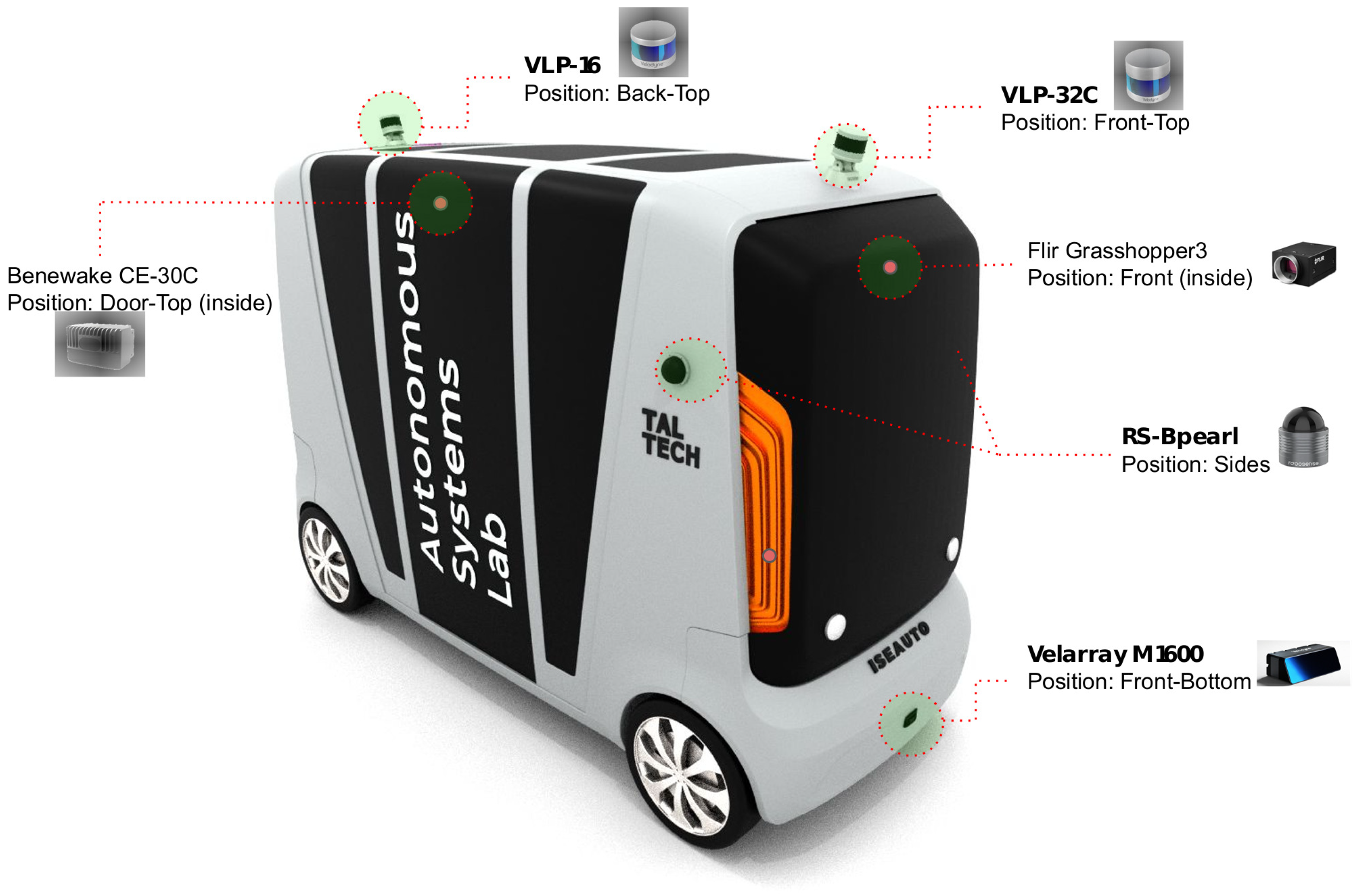
3.2.1. iseAuto Sensor Configuration

The sensor configurations of the iseAuto shuttle evolved along with the comprehensive practical tests [45]. The location of primary range sensors changed from two front-top corners to the middle of the front-top and back-top. Two 90${}^{\circ }$ vertical field-of-view (FoV) LiDARs on two sides of the shuttle were installed to cover the essential side-blind zones, especially in the proximity of door areas. Our latest upgrade is installing two solid-state LiDARs on the inside-door-top and outside-front-bottom for the door-movements safety and emergency brake, respectively. The main camera was installed inside the cabin, located in the front and behind the windshield. Figure 1 illustrates the positions and orientations of all perceptive sensors for the iseAuto shuttle.

In this work, the data collection was conducted by using the front-top Velodyne VLP-32C and front-inside FLIR Grasshopper3. As the two primary perceptive sensors for the iseAuto shuttle, the Velodyne VLP-32C has 32 channels that provide dense points clouds. The resolution of FLIR Grasshopper3 is up to 4240 × 2824 to guarantee a sharp vision of small objects such as traffic signs in the distance.

Table 1. Specifications of the primary camera and LiDAR sensors of the iseAuto shuttle.

	FoV (${}^{\circ }$)	Range (m)/Resolution	Update Rate (Hz)
Velodyne VLP-32C	40 (vertical)	200	20
Grasshopper3	89.3 (D) 77.3 (H) 61.7 (V)	4240 × 2824	7

contains detailed specifications of the camera and LiDAR sensors.

3.2.2. iseAuto Dataset Split

The environment of the iseAuto dataset is the TalTech campus, where the experimental campaign was conducted. Compared to the Waymo dataset used in the supervised learning baseline model, the night subset of the iseAuto data has a lower illumination condition. The ambient light of the campus is typically darker than the urban area where Waymo records their night data (shown in the first column of Figure 2). The partition of the iseAuto dataset follows the same principle as the Waymo dataset partitions, with four categories: day-fair, day-rain, night-fair, and night-rain. Both LiDAR and camera sensors were set to work at 7 Hz, which is the maximum frequency that the camera can shoot at 4k resolution. Correspondingly, one out of every seven frames of all point clouds and images were selected. To avoid the unbalanced data allocation that exists in the Waymon dataset (more data in day and fair conditions, less in night and rain), the total number of frames in each subset of the iseAuto dataset is 2000, to make sure that the same amount of knowledge can be gained from different weather and illumination conditions. For each subset, 600 frames were manually annotated with vehicle and human pixel-level classes. The data splits for training, early-stopping validation, and testing of all subsets have 300, 100, and 200 frames, respectively.

4. Methodology

Our work is an extension of the research presented in [9], where the authors differentiate the Waymo dataset by illumination (day/night) and weather (fair/rain) conditions to perform LiDAR–camera fusion and semi-supervised learning for semantic segmentation. We first follow the same principle to partition the Waymo dataset into four subsets (day-fair, day-rain, night-fair, and night-rain), then use them for the baseline model training. Secondly, we transfer the knowledge gained in the baseline supervised learning to the iseAuto dataset, in order to evaluate the network’s performance in new domains. At last, we conduct semi-supervised learning, which was expected to further improve the performance and domain adaptation. This section describes the data processing, model construction, and training procedures specifically designed for our work.

4.1. LiDAR Point Cloud Projection

One of the most common methods to process LiDAR data is converting 3D point clouds to 2D occupancy grids to efficiently exploit existing 2D convolutional networks. The late-fusion FCN used in this work requires both LiDAR and camera input as 2D images. Therefore, we apply perspective projection to project the point clouds into the camera plane for the Waymo and iseAuto datasets. This means that both LiDAR data and camera information need to be transformed into tensors. The usual procedure is to build n-2D tensors of a specific size (for instance, the input of the CNN); thus, the 3D LiDAR information should be projected into 2D tensors. For our case, the camera image tensor is $C_i\in {\mathbb{R}}^{h,w,3}$, where h is the height of the camera image, w is the width, and 3 is for the RGB color channels. Analogously, the LiDAR tensor is $L_i\in {\mathbb{R}}^{h,w,3}$, where h and w are the same height and width, and we use the three channels to represent the LiDAR data projection into the XY-YZ-ZX planes. The projection is carried out in a typical reference frame. For our case, the camera reference frame was chosen. Let $p_i^L={[x_i,y_i,z_i]}^T$ be the i-th point of the point cloud obtained as a LiDAR reading, in its own reference frame. Please observe that the reflective intensity value is ignored. The first step is to transform the point cloud from the LiDAR to the camera reference frame using a homogeneous transformation matrix, $p^C=T_C^L{p}^L$, where $p^C=[x,y,z,1]$ is a point represented in the camera reference frame, $p^L=[x,y,z]$ is a point represented in the LiDAR reference frame, and $T_C^L\in {\mathbb{R}}^{4,4}$ is the LiDAR–camera transformation matrix.

Now, it is possible to simply project each point in a 2D image, and thus each pixel value $(u,v)$ of a generic point $p_i$, where $u=1,\dots ,h$ is the row pixel coordinate, $v=1,\dots ,w$ is the column coordinate in pixels, and $h,w$ are the height and width of the camera image. Let R be the rectification matrix, and P the projection matrix; then, ${[u,v,1]}^T=PR{p}^C$.

The procedure above is applied to all points in the point clouds data. To ensure that the projected LiDAR plane has the same dimensions as the camera image, only the points within the field of view will be selected.

The Waymo dataset encodes the LiDAR data as range images with the same camera images format. Each pixel in the range image corresponds to a laser point reading. All the point information, such as range, vehicle pose, and camera projection, are included in the range image pixel. With the assistance of the toolkit, developers can directly extract point clouds images and well-overlaid camera projection from the Waymo dataset; thus, there no need to deal with the raw data.

For the iseAuto dataset, since the shuttle was operated upon by the robot operating system (ROS), LiDAR and camera data were captured as corresponding ROS formats and stored as the bag files. Pre-processes are needed to handle the point clouds and images. Extrinsic calibration of the LiDAR and camera first must be executed to compute the camera projection matrix and the LiDAR–camera transformation matrix. The rectification matrix was set to identity when projecting point clouds to images for the iseAuto dataset because rectification has been done internally by the camera. An example output of point clouds projection is shown in the second column of Figure 2. Note that the alignment of LiDAR points and image pixels is not ideal without extra operations to optimize the calibration and synchronization of LiDAR and camera sensors. Nevertheless, errors and interference always exist in the real world, which are the factors that we want to consider in this work through the iseAuto dataset.

4.2. Object Segmentation

Ground truth annotation is essential in machine learning and requires many labor costs. In the Waymo dataset, annotations were created separately for LiDAR and camera data. There are four kinds of objects (vehicles, pedestrians, signs, and cyclists) labeled in LiDAR sensor readings and three kinds of objects (vehicles, pedestrians, and cyclists) labeled in camera images. Both 3D and 2D annotations were represented by bounding boxes. Our process for the Waymo dataset is based on their LiDAR annotations. We select all LiDAR points within the 3D bounding box and project them into the image plane. Each projected point corresponds to a pixel in the image; the set of all projected points creates the semantic mask of the objects. Compared to the 2D annotations, the most important advantage of 3D annotations is that they provide a contour of the objects at a close distance. Correspondingly, the drawback of using 3D annotation is that some pixels in the semantic mask do not have labels because no LiDAR points fall into this area (see the third column of Figure 2).

The annotations of the iseAuto dataset were created based on camera images, as our high-resolution images contain more details of small objects (or objects that are far away). We develop a labeling tool that allows human annotators to draw objects’ contours in images and save the segmented area with its corresponding label. Semantic masks in the iseAuto dataset are flood-filled, which means all pixels in the mask have a unique label. Moreover, our annotations have an awareness of the contour of objects. It is a fact that human error is inevitable in manual labeling work. For scenarios with poor illumination conditions, point cloud projection was also used to identify possible objects that are not clearly visible in the camera image. For the scope of this work, the resolution of annotation images in the iseAuto dataset is 1920 × 1280; only vehicles and humans were masked out. Further work includes labeling higher-resolution images and more object classes. More objects and label verification are also needed.

Figure 2 shows some extracts of both datasets. The first row corresponds to the iseAuto dataset, while the second row shows the Waymo dataset. The comparison of the illumination condition in night scenarios is shown in the first column. Please note that, in similar scenes, the iseAuto dataset is typically darker than the Waymo dataset due to the external illumination and light source from the vehicle itself. The second column contains an example of the point clouds projection. The camera coordinate of points was used to pick out the corresponding pixels in the image. The colors of the pixels were assigned using the HSV palette, based on the depth information of the point. An upsampling process was used to make the iseAuto projection, as the point projection into a 4k resolution image is visually sparse. The third column illustrates the annotations of two datasets. As discussed above, no-label-zones exist in the Waymo dataset annotations because of the nature of LiDAR sensors. These areas must be excluded from the metrics calculation. The annotation of the iseAuto dataset is based on the camera image, in which the object masks are solid-filled and contain contour information.

4.3. Model

The model implemented in this work can be considered the composition of three different submodels. All of them are based on a well-known pre-trained ResNet50 [17] model. The first model works only on camera images with their respective labels. The second model has LiDAR data input instead. Lastly, the fusion model works as a joint combination of feature maps coming from the camera images and the LiDAR point clouds, which can be considered a late-fusion strategy. For each step, the loss function can be calculated at the output of each submodel. This strategy is further described in [9].

4.4. Training

There are three training procedures for transfer learning experiments. The first step is training supervised learning baseline models with only the Waymo dataset. The saved models in this step were tested separately by the Waymo and iseAuto datasets. The second procedure is the transfer learning experiment. Supervised learning baseline models of the Waymo were continuously trained by the iseAuto dataset. To assess the contribution of the knowledge attained from the Waymo dataset in the transfer learning process, there is also a training process to get iseAuto baseline models (trained by only the iseAuto dataset from scratch) in this step. The last procedure is semi-supervised learning (SSL). The literature is rich for SSL methods, such as the teacher-student model, co-training, or pseudo-labeling. Machine-made annotations of the unlabeled dataset were made by the transfer learning models from the Waymo to iseAuto dataset. Then unlabeled and labeled iseAuto data were mixed to continuously train the transfer learning models, and to train the iseAuto baseline model from scratch. Figure 3 summarily illustrates the training procedures that were mentioned above.

Cross-entropy loss fusion and Adam optimization [46] were used in this work. The hardware used for training is an Nvidia RTX2070 Super GPU. The batch size is 16. An early stopping mechanism was applied to all training processes. The learning rate decay follows the equation:

$$n(i)=n_0(1-\frac{i}{N}{)}^a$$

(1)

where the $n_0$ is the starting learning rate, a is 0.9, and N was denoted as the total iterations. Data augmentation was composed of random crop, random rotate, color jitter, and random horizontal and vertical flip. Figure 4 shows an example of the data augmentation. The output size of the random crop is 128 × 128. The random rotate range is (−20${}^{\circ }$, 20${}^{\circ }$), referring to the center of the images. The probability of executing the random vertical and horizontal is 50%. To maximize the diversity of the data augmentation, the order of the five augmentation processes was shuffled in every iteration. Remarkably, data normalization plays a vital role in this work, especially for the LiDAR data. Given the significant differences in specifications of the LiDAR sensors used in the Waymo and iseAuto datasets, the normalization of point clouds data of the two datasets has different factors. The $x,y,z$ coordinates of all points were appended together to compute mean and standard deviation values. Further fine-tuning to the normalization parameters was conducted to ensure the best performance.

4.5. Metrics

The measurements that were used to evaluate the performance of models include intersection over union (IoU), precision, recall, and area-under-curve average precision (auc-AP) [47].

IoU, also known as Jaccard index, is a measure to compare the similarity between two sample sets. The practical applications of IoU are mainly related to object detection, especially in the field of machine learning, to train a model to output boxes that fit around the objects. In this case, the ground-truth boxes (the hand-labeled bounding boxes that specify the location of the objects in the image) are needed to compute the IoU. The calculation is as follows:

$$\mathrm{IoU}=\frac{A_I}{A_U}$$

(2)

where $A_I$ is the overlap area, and $A_U$ is the union area of predicted and ground-truth boxes. The overlap and union area calculation is based on the image coordinates of the bounding box corners. However, our model produces instance segmentation of objects (per-pixel labeling), instead of bounding boxes. Therefore, we adopt a pixel-wise multi-class IoU algorithm to evaluate the model. Two object classes (vehicles and humans) were detected in this work. It was assumed that V represents the vehicle class and H represents the human class. The total number of pixels inferred as vehicle class (or human class) in both prediction and ground-truth was denoted as $V_p{V}_g$ (or $H_p{H}_g$). $V_p{H}_g$ represents the number of pixels indicated as a vehicle in prediction, but human in ground-truth. Similarly, $H_p{V}_g$ is the number of pixels labeled as human in prediction, but a vehicle in ground-truth. The IoU of two classes is attained by:

$${\mathrm{IoU}}_V=\frac{V_p{V}_g}{V_p{V}_g+V_p{H}_g+H_p{V}_g}$$

(3)

$${\mathrm{IoU}}_H=\frac{H_p{H}_g}{H_p{H}_g+H_p{V}_g+V_p{H}_g}.$$

(4)

Precision is a metric to reflect the model’s reliability in classifying samples as positive. It is defined as the ratio between the number of positive samples correctly classified and the total number of samples classified as positive (either correctly or incorrectly). In our case, the total number of pixels detected as vehicle or human by the model is the denominator of the precision calculation. Therefore, the precision of the two classes is given by the following equations:

$$\mathrm{Precision}\mathrm{of}\mathrm{vehicle}=\frac{V_p{V}_g}{V_p{V}_g+V_p{H}_g}$$

(5)

$$\mathrm{Precision}\mathrm{of}\mathrm{human}=\frac{H_p{H}_g}{H_p{H}_g+H_p{V}_g}$$

(6)

Recall indicates the capability of the model to detect the positive result. It is the ratio between the number of positive samples correctly classified as positive and the total number of positive samples. In our work, the recall of two classes is calculated by:

$$\mathrm{Recall}\mathrm{of}\mathrm{vehicle}=\frac{V_p{V}_g}{V_p{V}_g+H_p{V}_g}$$

(7)

$$\mathrm{Recall}\mathrm{of}\mathrm{human}=\frac{H_p{H}_g}{H_p{H}_g+V_p{H}_g}$$

(8)

In general, precision measures the capability of the model to classify the positive samples, but it does not consider correctly classifying all positive samples. On the contrary, recall measures the number of positive samples that the model correctly classified, but it neglects if the negative samples were classified as positive. High-precision-and-low-recall means that the model is reliable if it classifies a sample as positive, but only a few positive samples were classified. By contrast, low-precision-and-high-recall means most positive samples were correctly classified, but there are also many negative samples classified as positive by the model.

Plotting precision (y-axis) against recall (x-axis), named the precision-recall curve, is an efficient way to analyze the tradeoff between precision and recall at various thresholds. Average precision (AP) summarizes the information of a precision-recall curve into a single value. Typically, AP is defined as the area under the precision-recall curve between 0 and 1. In practice, the integral is simplified as the sum over the precision of different thresholds multiplied by the corresponding change in the recall. The auc-AP that was used in this work was proposed by PASCAL VOC 2010 [47], and it computes the AP as a numerical integration, with precision monotonically decreasing, by setting the precision for recall r to the maximum precision obtained for any recall $r^{\prime }\ge r$. The equation for computing auc-AP is:

$$\mathrm{auc}\text{\_}\mathrm{AP}=\sum _{k=1}^N\Delta r(k)\underset{\tilde{k}\ge k}{\max }p(\tilde{k})$$

(9)

5. Results and Discussion

As mentioned in Section 4.4, we conduct three training procedures in this work, which are described in this section and structured in the following way. We first evaluate the supervised learning baseline model of the Waymo dataset. Next, we analyze the transfer learning from the Waymo dataset to the iseAuto dataset. Finally, semi-supervised learning was applied for both iseAuto baseline and transfer learning models to assess its performance.

5.1. Waymo Supervised Learning Baseline

The Waymo supervised learning baseline models were trained by using all weather and illumination sequences of the Waymo dataset. As described in Section 3.1, the holdout method was used in the Waymo dataset to create the testing splits.

Table 2. Performance of supervised learning Waymo baseline models tested by the Waymo dataset.

		IoU (%)		Precision (%)		Recall (%)		auc-AP (%)
		Vehicle	Human	Vehicle	Human	Vehicle	Human	Vehicle	Human
Day-Fair	camera	88.08	55.57	91.21	59.77	96.25	88.77	92.60	71.13
	LiDAR	88.58	53.04	91.23	55.94	96.82	91.08	93.23	69.89
	fusion	91.07	62.50	93.05	65.16	97.72	93.87	94.35	76.05
Day-Rain	camera	88.54	52.13	91.14	57.43	96.88	84.97	94.04	76.12
	LiDAR	89.47	50.06	91.38	53.04	97.73	89.92	94.83	73.63
	fusion	92.77	64.66	94.35	68.53	98.23	91.97	95.80	84.55
Night-Fair	camera	81.16	42.87	86.77	49.33	92.62	76.60	86.74	61.10
	LiDAR	86.16	48.83	89.35	52.51	96.02	87.46	92.38	68.98
	fusion	89.41	60.33	91.96	65.08	97.00	89.22	92.18	73.02
Night-Rain	camera	74.49	43.14	83.39	51.91	87.47	71.87	85.83	53.04
	LiDAR	87.51	46.68	90.72	48.44	96.11	92.77	92.90	53.87
	fusion	89.90	56.70	92.86	60.84	96.58	89.28	94.52	66.81

refers to the result of the models trained and tested using the Waymo dataset only, corresponding to RGB, LiDAR, and fusion modes. This first test shows that our network compares well with other state-of-the-art works in terms of instance segmentation for the Waymo dataset [48,49]. Please note that this paper does not aim to outperform the Waymo benchmarks, but rather to analyze how much knowledge gained from the Waymo dataset can be transferred to a custom dataset to achieve good performance with only a limited amount of labeling work. Therefore, the same model trained by the Waymo dataset was tested by the iseAuto data without any additional training; the result is shown in

Table 3. Performance of supervised learning Waymo baseline models tested by the iseAuto dataset.

		IoU (%)		Precision (%)		Recall (%)		auc-AP (%)
		Vehicle	Human	Vehicle	Human	Vehicle	Human	Vehicle	Human
Day-Fair	camera	63.64	64.39	84.15	66.74	72.07	94.81	83.04	71.30
	LiDAR	40.56	0.06	63.19	57.87	53.12	0.06	49.68	0.35
	fusion	60.07	12.68	81.48	76.20	69.57	13.20	72.45	24.98
Day-Rain	camera	51.51	13.66	54.28	16.60	91.00	43.58	68.11	27.39
	LiDAR	43.56	2.86	67.96	11.96	54.81	3.62	51.98	7.62
	fusion	69.19	14.75	81.86	40.28	81.73	18.89	75.84	35.33
Night-Fair	camera	45.06	29.42	73.21	63.85	53.96	35.30	62.84	55.86
	LiDAR	41.75	0.54	56.92	20.72	61.04	0.55	48.20	1.61
	fusion	55.68	5.07	75.33	69.82	68.09	5.18	68.26	13.36
Night-Rain	camera	17.34	5.64	19.34	13.71	62.72	8.74	24.43	20.33
	LiDAR	33.55	0.01	48.09	0.33	52.59	0.01	41.26	0.08
	fusion	44.90	7.72	59.60	55.61	64.53	8.23	51.83	56.41

.

As the most represented class in the two datasets, the IoU and auc-AP of vehicles detection in the Waymo dataset reaches 93% and 96%, respectively. In the iseAuto dataset, the fusion model’s performance in vehicles detection is acceptable, ranging from 45% to 56% for IoU, and from 52% to 68% for auc-AP in challenging nighttime scenarios. By contrast, humans, which are smaller than vehicles in size and less represented in both datasets, show a lower segmentation accuracy than vehicles in the iseAuto dataset. Particularly for the LiDAR model, the performance degrades, as shown in Table 3. The knowledge gained from the Waymo LiDAR data seems to be less effective in detecting humans in the iseAuto dataset. This was expected due to the different LiDAR sensors used to capture the two datasets. It is not easy to compare data from various sensor technologies.

Specifically, in Table 2, precision values are lower than recall values (more significant difference for human class), which means that most of the objects were correctly classified. However, models also recognize some pixels belonging to other classes (e.g., background) as humans. In Table 3, it is the opposite: recall values are typically lower than precision values, which means that models cannot classify most of the objects correctly, but detection is relatively reliable. This shows that models trained by only the Waymo dataset realize the locations of the objects in the iseAuto dataset, but cannot draw out the whole object’s contour.

5.2. Transfer Learning to iseAuto

In the transfer learning experiment, supervised learning baseline models of Waymo were continuously trained using 1200 frames of iseAuto data that included different illumination and weather scenarios.

Table 4. Performance of the iseAuto transfer learning models from the Waymo dataset.

		IoU (%)		Precision (%)		Recall (%)		auc-AP (%)
		Vehicle	Human	Vehicle	Human	Vehicle	Human	Vehicle	Human
Day-Fair	camera	77.10	75.87	85.02	79.40	89.22	94.46	84.59	81.67
	LiDAR	72.14	55.71	81.07	57.48	86.75	94.75	80.65	61.08
	fusion	83.27	74.24	89.41	76.46	92.38	96.24	88.34	82.91
Day-Rain	camera	80.26	48.11	85.82	67.13	92.53	62.93	84.15	72.22
	LiDAR	77.33	40.27	82.35	45.06	92.70	79.11	81.48	63.36
	fusion	84.92	57.61	88.75	65.08	95.16	83.37	87.99	73.99
Night-Fair	camera	66.07	52.38	75.02	61.38	84.71	78.13	77.61	74.58
	LiDAR	74.50	45.38	80.58	47.78	90.79	90.04	82.93	60.75
	fusion	80.43	64.03	86.55	73.18	91.92	83.67	87.66	76.88
Night-Rain	camera	51.70	41.39	63.11	47.21	74.09	77.06	61.50	63.29
	LiDAR	62.51	26.46	68.24	27.05	88.15	92.38	73.02	50.79
	fusion	67.89	45.68	75.26	49.48	87.40	85.61	79.46	74.34

provides the metric results of the Waymo-to-iseAuto transfer learning models. For comparison, the same amount of iseAuto data was also used to train the iseAuto baseline models. The models’ performances are shown in

Table 5. Performance of the supervised learning iseAuto baseline models.

		IoU (%)		Precision (%)		Recall (%)		auc-AP (%)
		Vehicle	Human	Vehicle	Human	Vehicle	Human	Vehicle	Human
Day-Fair	camera	75.97	71.31	86.43	74.10	86.26	94.99	84.26	79.01
	LiDAR	71.19	56.87	78.74	59.01	88.14	94.03	78.00	66.99
	fusion	80.39	74.56	87.26	77.63	91.08	94.97	86.40	83.10
Day-Rain	camera	77.71	39.87	81.15	51.82	94.82	63.35	82.28	66.49
	LiDAR	76.00	42.10	81.44	46.52	91.93	81.58	80.43	59.12
	fusion	83.20	56.24	87.37	65.16	94.58	80.43	87.52	75.12
Night-Fair	camera	68.89	54.98	76.04	62.79	87.99	81.54	79.27	73.55
	LiDAR	74.25	47.19	80.03	50.52	91.13	87.75	82.96	54.16
	fusion	76.79	62.48	85.75	75.66	88.02	78.19	87.11	77.40
Night-Rain	camera	52.17	29.40	60.88	32.26	78.49	76.81	66.67	54.27
	LiDAR	59.49	36.76	64.82	37.91	87.85	92.33	82.30	62.08
	fusion	64.68	46.09	74.42	50.30	83.17	84.64	78.96	76.59

.

By comparing Table 4 and Table 5, one can note that, with the exception of human segmentation in the LiDAR model, all other metric results increase with transfer learning, as expected, even in challenging conditions such as night and rain. However, compared to the iseAuto baseline model, the transfer learning camera model significantly improves human segmentation, which results in the fusion model in the transfer learning process also generally performing better than the baseline. Please note that the amount of iseAuto data for training, 1200 frames in total, is much smaller than the Waymo data (16,188 frames) used for transfer learning and domain adaptation. The transfer learning fusion model has the best accuracy at this stage and is used to generate the machine-made labels for the unlabeled iseAuto data.

5.3. Semi-Supervised Learning with Pseudo-Labeled Data

Semi-supervised learning uses the unlabeled iseAuto dataset, applied to the iseAuto baseline models and Waymo-to-iseAuto transfer learning models. For each subset, there are 1400 frames of data labeled by the Waymo-to-iseAuto transfer learning fusion model (the best-performing model in earlier experiments). The machine-labeled data was mixed with human-labeled frames to perform the semi-supervised training. The same iseAuto data was used in all testing processes to ensure a parallel comparison. The evaluation of semi-supervised learning models is illustrated in

Table 6. Performance of the semi-supervised learning iseAuto baseline models.

		IoU (%)		Precision (%)		Recall (%)		auc-AP (%)
		Vehicle	Human	Vehicle	Human	Vehicle	Human	Vehicle	Human
Day-Fair	camera	79.85	67.06	85.27	68.18	92.63	97.62	85.86	75.88
	LiDAR	73.69	58.05	81.61	59.37	88.37	96.32	80.55	64.68
	fusion	82.38	68.98	87.24	69.98	93.67	97.96	87.72	76.36
Day-Rain	camera	80.27	53.61	82.57	56.91	96.64	90.24	84.41	67.23
	LiDAR	80.58	44.09	84.84	48.41	94.13	83.14	84.25	59.23
	fusion	83.98	54.28	87.13	56.95	95.87	92.06	88.63	66.87
Night-Fair	camera	73.14	55.07	78.67	61.71	91.23	83.66	81.74	69.23
	LiDAR	75.75	49.59	79.99	52.96	93.46	88.63	84.24	60.42
	fusion	79.28	56.32	82.34	59.81	95.52	90.61	86.68	71.81
Night-Rain	camera	60.42	42.06	66.33	43.80	87.16	91.37	69.26	68.97
	LiDAR	64.89	41.32	70.75	42.21	88.69	95.15	75.68	67.30
	fusion	63.97	43.63	69.38	44.74	89.13	94.59	75.67	67.84

and

Table 7. Performance of the semi-supervised transfer learning iseAuto models.

		IoU (%)		Precision (%)		Recall (%)		auc-AP (%)
		Vehicle	Human	Vehicle	Human	Vehicle	Human	Vehicle	Human
Day-Fair	camera	80.32	69.25	87.41	70.53	90.83	97.45	85.04	76.99
	LiDAR	76.10	61.81	83.28	63.30	89.83	96.34	81.32	71.22
	fusion	82.85	71.09	87.93	72.55	93.49	97.24	87.91	78.48
Day-Rain	camera	82.49	57.12	86.33	60.85	94.87	90.31	87.75	69.98
	LiDAR	81.00	44.85	85.03	49.57	94.48	82.50	85.05	60.68
	fusion	85.04	54.84	88.16	61.61	96.00	83.32	88.36	70.4
Night-Fair	camera	75.97	55.46	83.13	65.45	89.81	78.41	84.64	71.00
	LiDAR	76.01	51.63	80.16	55.07	93.63	89.20	84.01	64.51
	fusion	79.82	60.21	83.88	67.71	94.28	84.46	88.20	73.43
Night-Rain	camera	60.79	48.30	69.38	51.45	83.07	88.76	71.65	72.03
	LiDAR	64.40	41.15	69.95	42.17	89.04	94.45	73.63	64.49
	fusion	66.92	48.36	73.19	50.64	88.65	91.49	77.76	72.81

.

Referring to Table 6, the semi-supervised learning iseAuto baseline models show 84% IoU and 89% auc-AP for vehicle segmentation in fair illumination and weather conditions. By comparing Table 5 and Table 6, it is possible to see that the vehicle segmentation shows robust performance improvement even in more challenging scenarios with the help of the semi-supervised learning. The human segmentation is a weak point in this stage, which can be explained by the fact that the humans class is less represented in the dataset; too few human samples are being recorded in the iseAuto dataset. Please note that recall shows an effective increase in semi-supervised learning baseline models, which means that there is an improvement of the models’ capability to detect the positive human samples. This corresponds to the general principle in machine learning that more data can bring higher performance. While there is a minor decline in precision, which means models detect more negative samples as the human class, it proves the extra unlabeled data increases the model’s uncertainty about the human class in semi-supervised learning.

Table 7 evaluates the semi-supervised learning iseAuto models with the transfer learning knowledge from the Waymo dataset. The best-performing Waymo supervised learning baseline models were continuously trained by full-annotated iseAuto dataset. Comparing the results to Table 6, major improvement can be seen in all modalities and domains, which means the knowledge gained from the Waymo dataset is still valuable for the semi-supervised learning stage. Compared to the transfer learning iseAuto models without semi-supervised learning (Table 4), the individual RGB and LiDAR networks have a maximum of 10% increase in some cases. At the same time, the fusion model does not show further improvement with additional machine-annotated data in training. This effect is more evident in challenging scenarios with the human class. The reason might be attributed to a lack of accuracy in the labels, particularly in the semi-supervised learning mode, and a scarcity of data points for smaller objects, such as a human.

In summary, through all the above scenarios, it is possible to say that domain adaptation and semi-supervised learning can lead to an average increase between 2 to 5 percentage points in vehicle segmentation. Specifically, in the average of all above scenarios, vehicle segmentation in fusion mode improves from 76% in the iseAuto baseline to 79% in the semi-supervised transfer learning mode, an increase of three percentage points. However, accurately segmenting less-represented classes with fewer points in the scenario, such as the human class, remains a challenge due to the scarcity of data and inaccurate machine labeling.

6. Conclusions

In this paper, the results of our machine learning algorithm involving LiDAR–camera fusion, transfer learning, and semi-supervised learning on our custom dataset are shown. The data used in this work are acquired using our custom autonomous shuttle, iseAuto. This work extends the results presented in a previous conference paper by giving a deep insight and analysis of the performance of our machine learning algorithm. Our algorithm’s performance is first shown on a publicly available dataset, the Waymo data, used as a benchmark to show that this algorithm is aligned with the state of the art. As the main focus of this paper is to show that it is possible to achieve reasonable performance on a custom dataset with only a limited amount of annotation, we have trained the network with little data (only 10% of Waymo), showing an already reasonable performance. The baseline was compared against a network trained on Waymo and combining iseAuto data in transfer learning, providing over 80% performance in IoU in day-fair conditions and using the fusion algorithm. In the future, this work can be extended by adding more labeled and unlabeled data to the iseAuto dataset with more diversity for different weather conditions and traffic scenarios, and including more classes. The performance of the fusion model has enormous potential to be further improved. A different line of work could be adaptation research of our algorithms for different dataset sources to improve the networks’ capability in domain adaptation and detecting more challenging object classes.

References

1. Liu, W.; Anguelov, D.; Erhan, D.; Szegedy, C.; Reed, S.; Fu, C.Y.; Berg, A.C. Ssd: Single shot multibox detector. In European Conference on Computer Vision; Springer: Berlin/Heidelberg, Germany, 2016; pp. 21–37. [Google Scholar]
2. Ren, S.; He, K.; Girshick, R.; Sun, J. Faster r-cnn: Towards real-time object detection with region proposal networks. IEEE Trans. Pattern Anal. Mach. Intell. 2015, 39, 1137–1149. [Google Scholar] [CrossRef] [PubMed] [Green Version]
3. He, K.; Gkioxari, G.; Dollár, P.; Girshick, R. Mask r-cnn. In Proceedings of the 2017 IEEE Transactions on Pattern Analysis and Machine Intelligence, Venice, Italy, 22–29 October 2017; pp. 386–397. [Google Scholar]
4. Milioto, A.; Vizzo, I.; Behley, J.; Stachniss, C. Rangenet++: Fast and accurate lidar semantic segmentation. In Proceedings of the 2019 IEEE/RSJ International Conference on Intelligent Robots and Systems (IROS), Macau, China, 3–8 November 2019; pp. 4213–4220. [Google Scholar]
5. Qi, C.R.; Yi, L.; Su, H.; Guibas, L.J. Pointnet++: Deep hierarchical feature learning on point sets in a metric space. In Proceedings of the 31st International Conference on Neural Information Processing Systems, Red Hook, NY, USA, 4–9 December 2017. [Google Scholar]
6. Caltagirone, L.; Bellone, M.; Svensson, L.; Wahde, M. LIDAR-Camera fusion for road detection using fully convolutional neural networks. Robot. Auton. Syst. 2019, 111, 125–131. [Google Scholar] [CrossRef] [Green Version]
7. Pang, S.; Morris, D.; Radha, H. CLOCs: Camera-LiDAR object candidates fusion for 3D object detection. In Proceedings of the 2020 IEEE/RSJ International Conference on Intelligent Robots and Systems (IROS), Las Vegas, NV, USA, 24 October–24 January 2021; pp. 10386–10393. [Google Scholar]
8. Van Gansbeke, W.; Neven, D.; De Brabandere, B.; Van Gool, L. Sparse and noisy lidar completion with rgb guidance and uncertainty. In Proceedings of the 2019 16th International Conference on Machine Vision Applications (MVA), Tokyo, Japan, 27–31 May 2019; pp. 1–6. [Google Scholar]
9. Caltagirone, L.; Bellone, M.; Svensson, L.; Wahde, M.; Sell, R. LiDAR-Camera Semi-Supervised Learning for Semantic Segmentation. Sensors 2021, 21, 4813. [Google Scholar] [CrossRef] [PubMed]
10. Geiger, A.; Lenz, P.; Stiller, C.; Urtasun, R. Vision meets robotics: The kitti dataset. Int. J. Robot. Res. 2013, 32, 1231–1237. [Google Scholar] [CrossRef] [Green Version]
11. Sun, P.; Kretzschmar, H.; Dotiwalla, X.; Chouard, A.; Patnaik, V.; Tsui, P.; Guo, J.; Zhou, Y.; Chai, Y.; Caine, B.; et al. Scalability in perception for autonomous driving: Waymo open dataset. In Proceedings of the 2020 IEEE/CVF Conference on Computer Vision and Pattern Recognition (CVPR), Seattle, WA, USA, 16–18 June 2020; pp. 2443–2451. [Google Scholar]
12. Chang, M.F.; Lambert, J.; Sangkloy, P.; Singh, J.; Bak, S.; Hartnett, A.; Wang, D.; Carr, P.; Lucey, S.; Ramanan, D.; et al. Argoverse: 3D Tracking and Forecasting with Rich Maps. In Proceedings of the 2019 IEEE/CVF Conference on Computer Vision and Pattern Recognition (CVPR), Long Beach, CA, USA, 15–20 June 2019; pp. 8740–8749. [Google Scholar]
13. Caesar, H.; Bankiti, V.; Lang, A.H.; Vora, S.; Liong, V.E.; Xu, Q.; Krishnan, A.; Pan, Y.; Baldan, G.; Beijbom, O. Nuscenes: A multimodal dataset for autonomous driving. In Proceedings of the 2020 IEEE/CVF Conference on Computer Vision and Pattern Recognition (CVPR), Seattle, WA, USA, 16–18 June 2020; pp. 11621–11631. [Google Scholar]
14. Sell, R.; Leier, M.; Rassõlkin, A.; Ernits, J.P. Self-driving car ISEAUTO for research and education. In Proceedings of the 2018 19th International Conference on Research and Education in Mechatronics (REM), Delft, The Netherlands, 7–8 June 2018; pp. 111–116. [Google Scholar]
15. Rassõlkin, A.; Gevorkov, L.; Vaimann, T.; Kallaste, A.; Sell, R. Calculation of the traction effort of ISEAUTO self-driving vehicle. In Proceedings of the 2018 25th International Workshop on Electric Drives: Optimization in Control of Electric Drives (IWED), Moscow, Russia, 31 January–2 February 2018; pp. 1–5. [Google Scholar]
16. Sell, R.; Rassõlkin, A.; Wang, R.; Otto, T. Integration of autonomous vehicles and Industry 4.0. Proc. Est. Acad. Sci. 2019, 68, 389–394. [Google Scholar] [CrossRef]
17. He, K.; Zhang, X.; Ren, S.; Sun, J. Deep residual learning for image recognition. In Proceedings of the 2016 IEEE Conference on Computer Vision and Pattern Recognition (CVPR), Las Vegas, NV, USA, 27–30 June 2016; pp. 770–778. [Google Scholar]
18. Bellone, M.; Ismailogullari, A.; Müür, J.; Nissin, O.; Sell, R.; Soe, R.M. Autonomous driving in the real-world: The weather challenge in the Sohjoa Baltic project. In Towards Connected and Autonomous Vehicle Highways; Springer: Berlin/Heidelberg, Germany, 2021; pp. 229–255. [Google Scholar]
19. Brostow, G.J.; Fauqueur, J.; Cipolla, R. Semantic object classes in video: A high-definition ground truth database. Pattern Recognit. Lett. 2009, 30, 88–97. [Google Scholar] [CrossRef]
20. Geyer, J.; Kassahun, Y.; Mahmudi, M.; Ricou, X.; Durgesh, R.; Chung, A.S.; Hauswald, L.; Pham, V.H.; Mühlegg, M.; Dorn, S.; et al. A2d2: Audi autonomous driving dataset. arXiv 2004, arXiv:2004.06320. [Google Scholar]
21. Jeong, J.; Cho, Y.; Shin, Y.S.; Roh, H.; Kim, A. Complex urban dataset with multi-level sensors from highly diverse urban environments. Int. J. Robot. Res. 2019, 38, 642–657. [Google Scholar] [CrossRef] [Green Version]
22. Behrendt, K.; Soussan, R. Unsupervised labeled lane markers using maps. In Proceedings of the 2019 IEEE/CVF International Conference on Computer Vision Workshop (ICCVW), Seoul, Korea, 27 October–2 November 2019; pp. 832–839. [Google Scholar]
23. Huang, X.; Wang, P.; Cheng, X.; Zhou, D.; Geng, Q.; Yang, R. The apolloscape open dataset for autonomous driving and its application. IEEE Trans. Pattern Anal. Mach. Intell. 2019, 42, 2702–2719. [Google Scholar] [CrossRef] [PubMed] [Green Version]
24. Van Engelen, J.E.; Hoos, H.H. A survey on semi-supervised learning. Mach. Learn. 2020, 109, 373–440. [Google Scholar] [CrossRef] [Green Version]
25. Yang, X.; Song, Z.; King, I.; Xu, Z. A survey on deep semi-supervised learning. arXiv 2021, arXiv:2103.00550. [Google Scholar]
26. Miller, D.J.; Uyar, H. A mixture of experts classifier with learning based on both labelled and unlabelled data. In Proceedings of the 9th International Conference on Neural Information Processing Systems, Cambridge, MA, USA, 3–5 December 1996. [Google Scholar]
27. Shahshahani, B.M.; Landgrebe, D.A. The effect of unlabeled samples in reducing the small sample size problem and mitigating the Hughes phenomenon. IEEE Trans. Geosci. Remote Sens. 1994, 32, 1087–1095. [Google Scholar] [CrossRef] [Green Version]
28. Joachims, T. Transductive inference for text classification using support vector machines. In Proceedings of the Sixteenth International Conference on Machine Learning (ICML), Bled, Slovenia, 27–30 June 1999; Volume 99, pp. 200–209. [Google Scholar]
29. Belkin, M.; Niyogi, P.; Sindhwani, V. Manifold regularization: A geometric framework for learning from labeled and unlabeled examples. J. Mach. Learn. Res. 2006, 7, 2399–2434. [Google Scholar]
30. Blum, A.; Mitchell, T. Combining labeled and unlabeled data with co-training. In Proceedings of the Eleventh Annual Conference on Computational Learning Theory, Madison, WI, USA, 24–26 July 1998; pp. 92–100. [Google Scholar]
31. Agrawala, A. Learning with a probabilistic teacher. IEEE Trans. Inf. Theory 1970, 16, 373–379. [Google Scholar] [CrossRef] [Green Version]
32. Zhu, Y.; Zhang, Z.; Wu, C.; Zhang, Z.; He, T.; Zhang, H.; Manmatha, R.; Li, M.; Smola, A. Improving semantic segmentation via self-training. arXiv 2020, arXiv:2004.14960. [Google Scholar] [CrossRef]
33. Cordts, M.; Omran, M.; Ramos, S.; Rehfeld, T.; Enzweiler, M.; Benenson, R.; Franke, U.; Roth, S.; Schiele, B. The cityscapes dataset for semantic urban scene understanding. In Proceedings of the IEEE Conference on Computer Vision and Pattern Recognition, Las Vegas, NV, USA, 27–30 June 2016; pp. 3213–3223. [Google Scholar]
34. Brostow, G.J.; Shotton, J.; Fauqueur, J.; Cipolla, R. Segmentation and recognition using structure from motion point clouds. In European Conference on Computer Vision; Springer: Berlin/Heidelberg, Germany, 2008; pp. 44–57. [Google Scholar]
35. Xie, Q.; Luong, M.T.; Hovy, E.; Le, Q.V. Self-training with noisy student improves imagenet classification. In Proceedings of the 2020 IEEE/CVF Conference on Computer Vision and Pattern Recognition (CVPR), Seattle, WA, USA, 16–18 June 2020; pp. 10684–10695. [Google Scholar]
36. Zhai, X.; Oliver, A.; Kolesnikov, A.; Beyer, L. S4l: Self-supervised semi-supervised learning. In Proceedings of the 2019 IEEE/CVF International Conference on Computer Vision (ICCV), Seoul, Korea, 27 October–2 November 2019; pp. 1476–1485. [Google Scholar]
37. Ma, F.; Cavalheiro, G.V.; Karaman, S. Self-supervised sparse-to-dense: Self-supervised depth completion from lidar and monocular camera. In Proceedings of the 2019 International Conference on Robotics and Automation (ICRA), Montreal, QC, Canada, 20–24 May 2019; pp. 3288–3295. [Google Scholar]
38. Park, K.; Kim, S.; Sohn, K. High-precision depth estimation using uncalibrated LiDAR and stereo fusion. IEEE Trans. Intell. Transp. Syst. 2019, 21, 321–335. [Google Scholar] [CrossRef]
39. Xu, D.; Anguelov, D.; Jain, A. Pointfusion: Deep sensor fusion for 3d bounding box estimation. In Proceedings of the 2018 IEEE/CVF Conference on Computer Vision and Pattern Recognition, Salt Lake City, UT, USA, 18–23 June 2018; pp. 244–253. [Google Scholar]
40. Qi, C.R.; Su, H.; Mo, K.; Guibas, L.J. Pointnet: Deep learning on point sets for 3d classification and segmentation. In Proceedings of the 2017 IEEE Conference on Computer Vision and Pattern Recognition (CVPR), Honolulu, HI, USA, 21–26 June 2017; pp. 77–85. [Google Scholar]
41. Liang, M.; Yang, B.; Chen, Y.; Hu, R.; Urtasun, R. Multi-task multi-sensor fusion for 3d object detection. In Proceedings of the 2019 IEEE/CVF Conference on Computer Vision and Pattern Recognition (CVPR), Long Beach, CA, USA, 16–20 June 2019; pp. 7337–7345. [Google Scholar]
42. Su, H.; Jampani, V.; Sun, D.; Maji, S.; Kalogerakis, E.; Yang, M.H.; Kautz, J. Splatnet: Sparse lattice networks for point cloud processing. In Proceedings of the 2018 IEEE/CVF Conference on Computer Vision and Pattern Recognition, Salt Lake City, UT, USA, 18–23 June 2018; pp. 2530–2539. [Google Scholar]
43. Bai, M.; Mattyus, G.; Homayounfar, N.; Wang, S.; Lakshmikanth, S.K.; Urtasun, R. Deep multi-sensor lane detection. In Proceedings of the 2018 IEEE/RSJ International Conference on Intelligent Robots and Systems (IROS), Madrid, Spain, 1–5 October 2018; pp. 3102–3109. [Google Scholar]
44. Chen, Z.; Zhang, J.; Tao, D. Progressive lidar adaptation for road detection. IEEE/CAA J. Autom. Sin. 2019, 6, 693–702. [Google Scholar] [CrossRef] [Green Version]
45. Gu, J.; Chhetri, T.R. Range Sensor Overview and Blind-Zone Reduction of Autonomous Vehicle Shuttles. In IOP Conference Series: Materials Science and Engineering; IOP Publishing: Bristol, UK, 2021; Volume 1140, p. 012006. [Google Scholar]
46. Kingma, D.P.; Ba, J. Adam: A method for stochastic optimization. arXiv 2014, arXiv:1412.6980. [Google Scholar]
47. Everingham, M.; Van Gool, L.; Williams, C.K.I.; Winn, J.; Zisserman, A. The PASCAL Visual Object Classes Challenge 2010 (VOC2010) Results. Available online: http://www.pascal-network.org/challenges/VOC/voc2010/workshop/index.html (accessed on 17 December 2021).
48. Jiang, C.; Xu, H.; Zhang, W.; Liang, X.; Li, Z. Sp-nas: Serial-to-parallel backbone search for object detection. Proceedings of 2020 IEEE/CVF Conference on Computer Vision and Pattern Recognition (CVPR), Seattle, WA, USA, 16–18 June 2020; pp. 11860–11869. [Google Scholar]
49. Zhang, Y.; Song, X.; Bai, B.; Xing, T.; Liu, C.; Gao, X.; Wang, Z.; Wen, Y.; Liao, H.; Zhang, G.; et al. 2nd Place Solution for Waymo Open Dataset Challenge–Real-time 2D Object Detection. arXiv 2021, arXiv:2106.08713. [Google Scholar]
Figure 1. Perceptive sensors layout. The Benewake CE-30C LiDAR is located inside the shuttle and attached on top of the door.
Electronics 11 01119 g001
Figure 2. Extract from the iseAuto dataset (ac) on the first row; the second row represents the Waymo dataset (df). For additional details, please refer to Section 4.
Electronics 11 01119 g002
Figure 3. The workflow of the training procedures. ‘TL’ and ‘SSL’ stand for transfer learning and semi-supervised learning, respectively. ‘Waymo labeled splits’ and ‘iseAuto labeled splits’ represent the Waymo and iseAuto manual-labeled data. ‘iseAuto unlabeled splits’ means the iseAuto machine-labeled data produced by the iseAuto transfer learning fusion model. ‘Waymo baseline models’ and ‘iseAuto baseline models’ stand for supervised learning baseline models of the the Waymo and iseAuto dataset. ‘iseAuto TL models’ means the Waymo-to-iseAuto transfer learning models. ‘iseAuto SSL-TL models’ and ‘iseAuto SSL models’ are iseAuto semi-supervised learning models with and without knowledge adapted from the Waymo dataset, respectively. Please refer to Section 4.4 for further details.
Electronics 11 01119 g003
Figure 4. Data augmentation processes: (a) is the original image, (b) is color jitter, (c) is horizontal flip, (d) is random rotate in the range (−20 , 20 ), (e) is the random crop of dimension 128 × 128.
Electronics 11 01119 g004