
Maximizing Channel Capacity of 3D MIMO System via Antenna Downtilt Angle Adaptation Using a Q-Learning Algorithm


Abstract
:1. Introduction
2. System Model and Q-Learning Algorithm
2.1. MIMO System Architecture
2.2. Maximum Channel Entropy
2.3. Calculation of 3D MIMO Channel Capacity
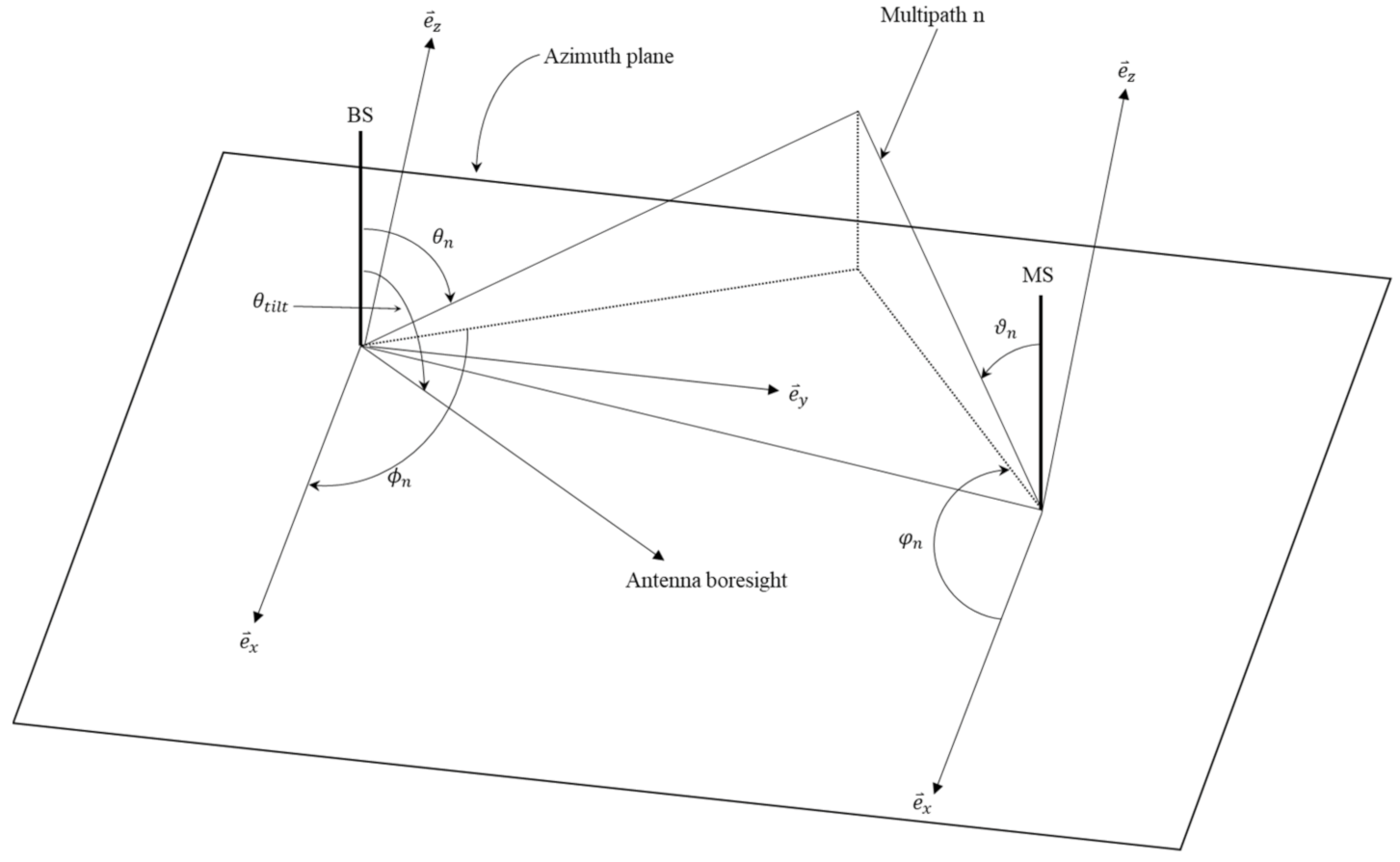
2.3.1. Elevation Angle between Transmitting and Receiving Path (AoDs, AoAs)
2.3.2. Antenna Downtilt Angle and Elevation Angle of Line of Sight
2.3.3. Channel Capacity
2.4. The Effect of Antenna Downtilt Angle on Channel Capacity
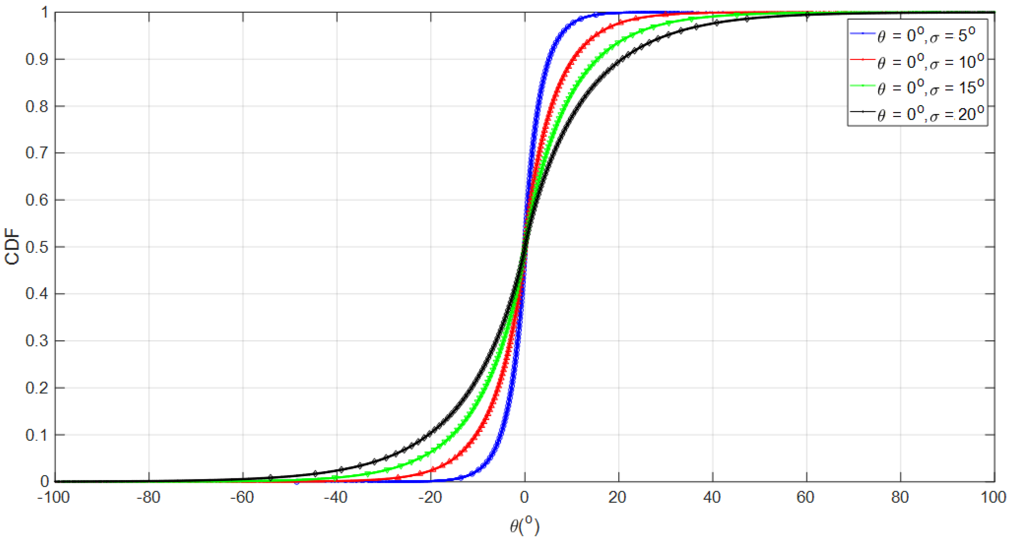
2.4.1. Distributions of EAoDs and EAoAs
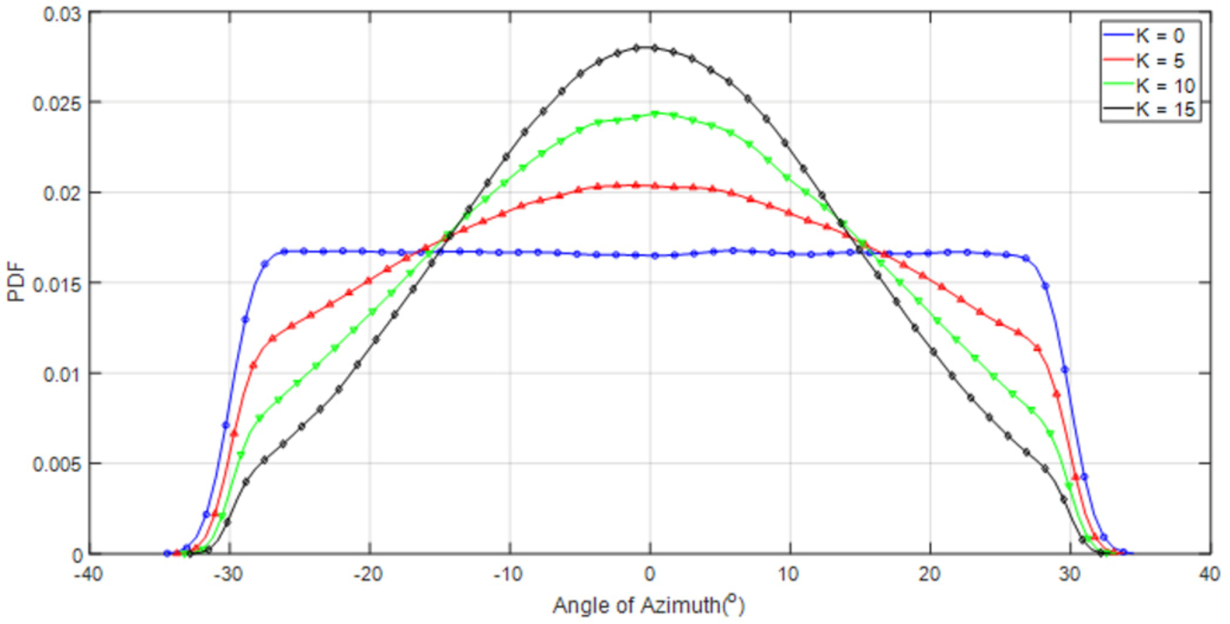
2.4.2. Distributions of AAoDs and AAoAs
2.4.3. Simulation Parameters with Different Antenna Downtilt Angles
2.5. Q-Learning Algorithm
3. Adaptive Optimization of Antenna Downtilt Angle Based on the Q-Learning Algorithm
3.1. Simulation Procedure with the Q-Learning Algorithm
- 1.
- In order to understand all states first and then set the reward value, the search angle is between 90°–125°, and the interval is 0.5 degrees, so a total of 71 angles need to be searched.
- 1.
- Calculate the channel capacity at each angle.
- 1.
- Set the parameters in Equation (24).
- 4.
- The initial environment is unknown and the initial Q matrix is a 71 × 71 zero matrix because it has not been iterated,
- 5.
- Build R (reward matrix), cn: channel capacity at the nth angle.
- 6.
- of all possible actions in Angle (state, ) moving to the next Angle (state, ): select the action () that can obtain the maximum Q value after performing, and multiply the maximum Q value by γ.
- 7.
- Iterative process: randomly select the angle (state, ) to perform the action (), obtain the reward value (R(, )), and then move from the angle (state, ) to the next angle (state, ). Among all possible actions , the maximum Q value is multiplied by γ to iterate, and the Q table can be obtained after the iteration.
- 8.
- The angle (state) corresponding to the optimal Q value in the search Q matrix is the optimal antenna downtilt angle.
3.2. Ideal Optimal Channel Capacity Based on Ideal Condition
3.2.1. Channel Capacity of 20 × 1 Antenna Configuration at
3.2.2. Channel Capacity of 60 × 4 Antenna Configuration at
4. Results and Discussion
4.1. Optimized Channel Capacity of 20 × 1 Antenna Configuration Based on
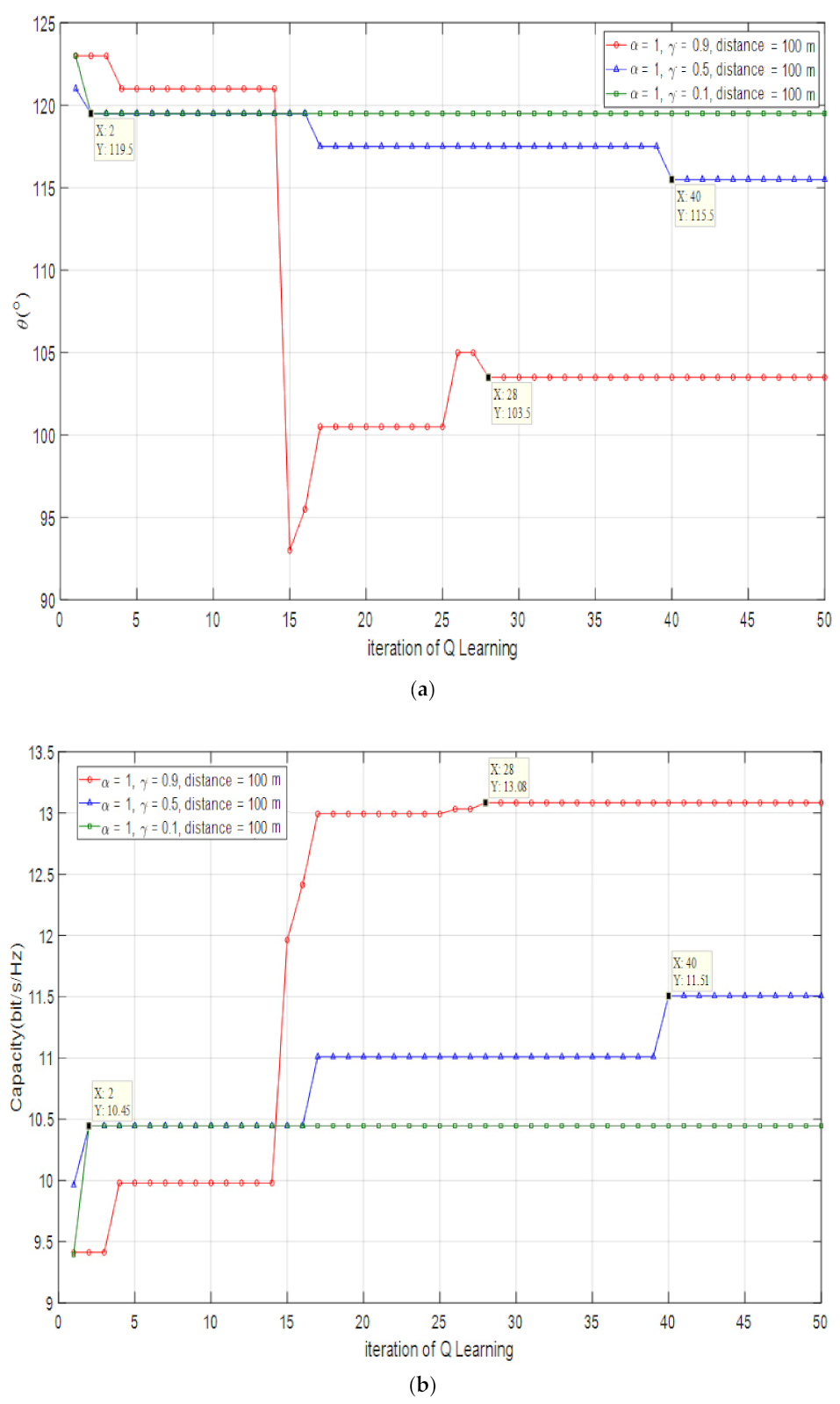
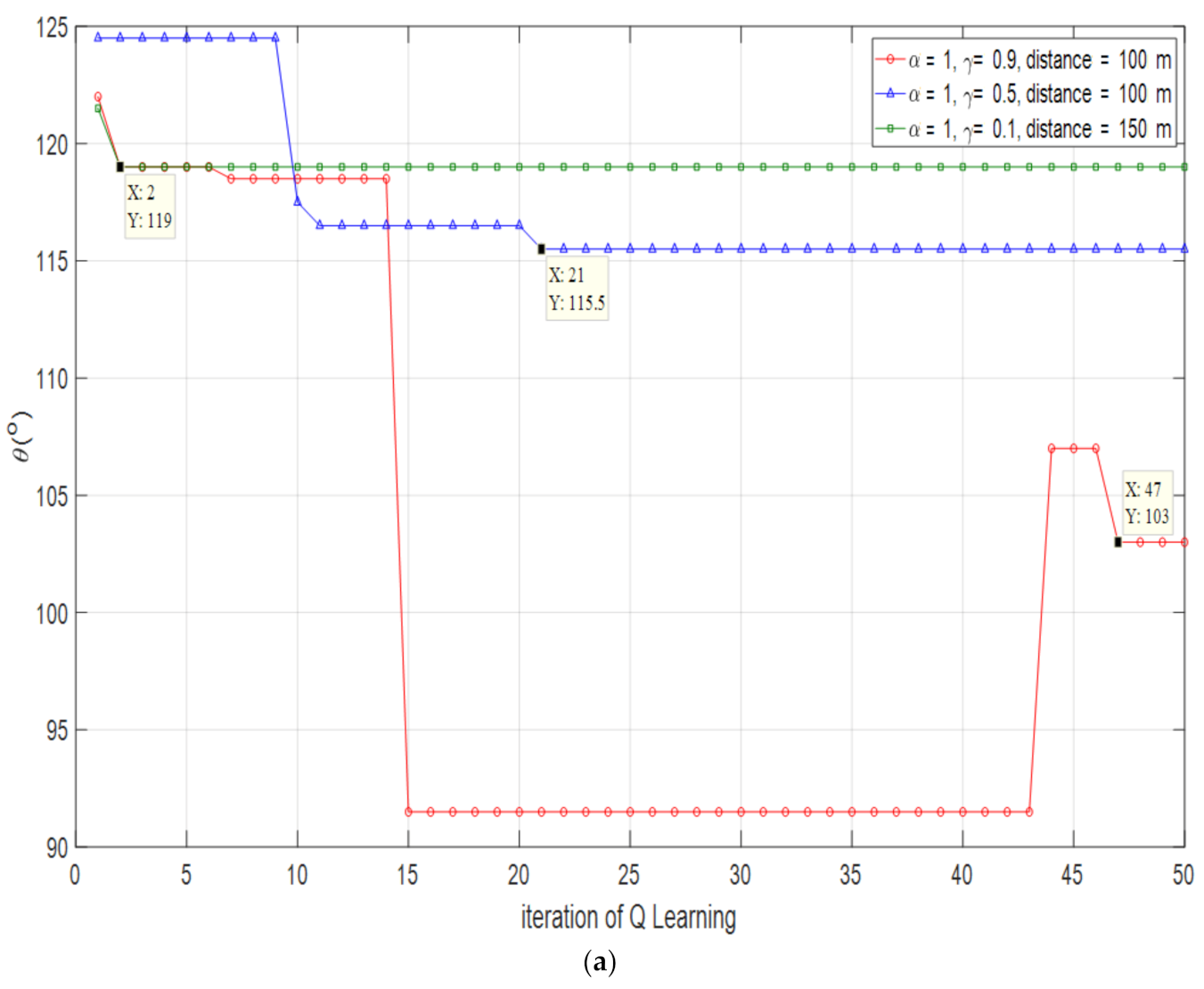
4.1.1. Optimized Channel Capacity and Optimized at D = 100 m
4.1.2. Optimized Channel Capacity and Optimized at D = 150 m
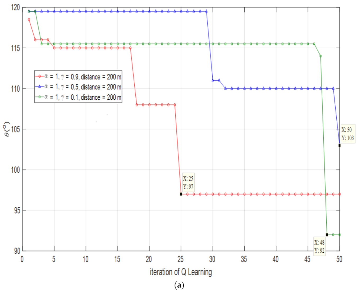
4.1.3. Optimized Channel Capacity and Optimized at D = 200 m
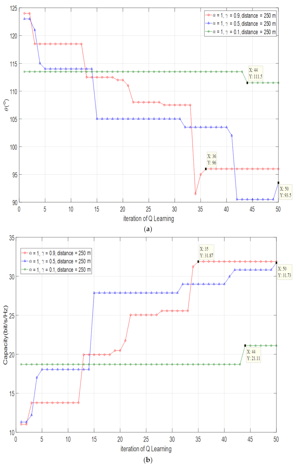
4.1.4. Optimized Channel Capacity and Optimized at D = 250 m
4.2. Optimized Channel Capacity of 60 × 4 Antenna Configuration Based on Adaptive
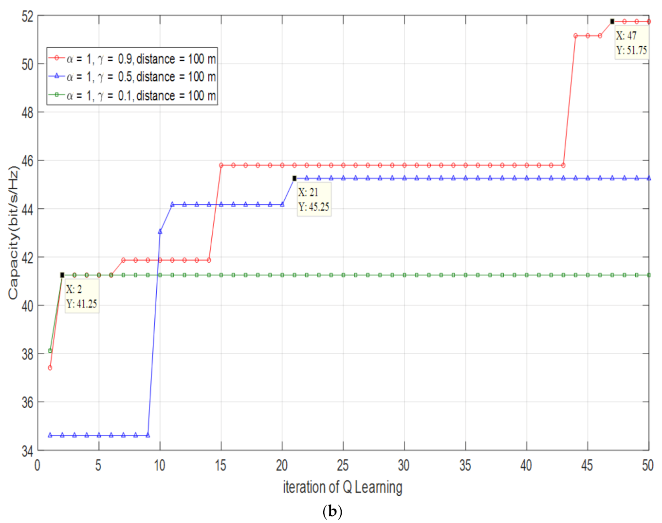
4.2.1. Optimized Channel Capacity and Optimized at D = 100 m
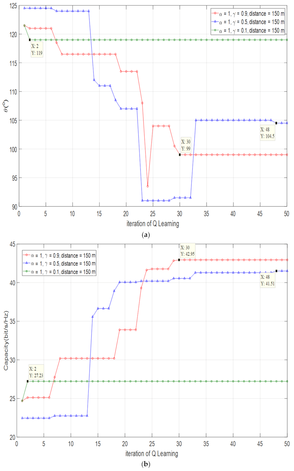
4.2.2. Optimized Channel Capacity and Optimized at D = 150 m
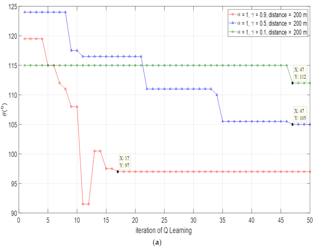
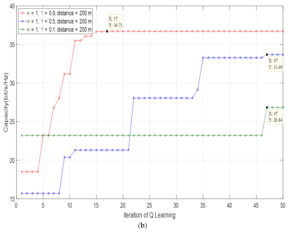
4.2.3. Optimized Channel Capacity and Optimized at D = 200 m
4.2.4. Optimized Channel Capacity and Optimized at D = 250 m
5. Conclusions
Author Contributions
Funding
Conflicts of Interest
References
- Chen, J.; Qian, Z.; Wang, T.; Li, X. Analysis on the protection distance for spectrum sharing between IMT-2020(5G) and EESS systems in 25.5–27GHz band. In Proceedings of the 2017 IEEE 2nd Information Technology, Networking, Electronic and Automation Control Conference (ITNEC), Chengdu, China, 15–17 December 2017; pp. 970–975. [Google Scholar] [CrossRef]
- Tanveer, J.; Haider, A.; Ali, R.; Kim, A. Machine Learning for Physical Layer in 5G and beyond Wireless Networks: A Survey. Electronics 2022, 11, 121. [Google Scholar] [CrossRef]
- Roshanzamir, A.; Bastani, M.H.; Roshanzamir, M. Analysing of 3D beamforming in MIMO radars. In Proceedings of the 2012 World Congress on Information and Communication Technologies, Trivandrum, India, 30 October–2 November 2012; pp. 745–749. [Google Scholar] [CrossRef]
- Qurrat-Ul-Ain, N.; Abla, K.; Mérouane, D. Design of 5G Full Dimension Massive MIMO Systems. IEEE Trans. Commun. 2017, 66, 726–740. [Google Scholar]
- Zhang, W.; Wang, Y.; Peng, F.; Yuan, Y. Interference Coordination with Vertical Beamforming in 3D MIMO-OFDMA Networks. IEEE Commun. Lett. 2014, 18, 34–37. [Google Scholar] [CrossRef]
- Kulin, M.; Kazaz, T.; De Poorter, E.; Moerman, I. A Survey on Machine Learning-Based Performance Improvement of Wireless Networks: PHY, MAC and Network Layer. Electronics 2021, 10, 318. [Google Scholar] [CrossRef]
- Huang, Y.-F.; Lin, C.-B.; Chung, C.-M.; Chen, C.-M. Research on QoS Classification of Network Encrypted Traffic Behavior Based on Machine Learning. Electronics 2021, 10, 1376. [Google Scholar] [CrossRef]
- Shen, H.; Zhang, Y.; Mao, J.; Yan, Z.; Wu, L. Energy Management of Hybrid UAV Based on Reinforcement Learning. Electronics 2021, 10, 1929. [Google Scholar] [CrossRef]
- Sutton, R.S.; Barto, A.G. Reinforcement Learning: An Introduction, 2nd ed.; The MIT Press: Cambridge, MA, USA, 2017. [Google Scholar]
- Watkins, C.J.C.H.; Dayan, P. Q-learning. Mach. Learn. 1992, 8, 279–292. [Google Scholar] [CrossRef]
- Nadeem, Q.-U.; Kammoun, A.; Debbah, M.; Alouini, M.-S. 3D Massive MIMO Systems: Modeling and Performance Analysis. IEEE Trans. Wirel. Commun. 2015, 14, 6926–6939. [Google Scholar] [CrossRef] [Green Version]
- Zhang, J.; Pan, C.; Pei, F.; Liu, G.; Cheng, X. Three-dimensional fading channel models: A survey of elevation angle research. IEEE Commun. Mag. 2014, 52, 218–226. [Google Scholar] [CrossRef]
- GPP. Study on 3D Channel Model for Elevation Beamforming and FD-MIMO Studies for LTE; 3GPP: Sophia Antipolis, France, 2012. [Google Scholar]
- HUAWEI. White Paper. 4.5G, Opening Giga Mobile World, Empowering Vertical Markets; Huawei Technologies: Shenzhen, China, 2016. [Google Scholar]
- Baum, D.; Hansen, J.; Salo, J.; Galdo, G.; Milojevic, M.; Kyosti, P. An Interim Channel Model for Beyond-3G Systems Extending the 3GPP Spatial Channel Model (SCM). In Proceedings of the IEEE 61st Vehicular Technology Conference, Stockholm, Sweden, 30 May–1 June 2005. [Google Scholar] [CrossRef]
- Döttling, M.; Mohr, W.; Osseiran, A. WINNER II Channel Models. In Radio Technologies and Concepts for IMT-Advanced; Wiley Telecom: Oxford, UK, 2010; pp. 39–92. [Google Scholar] [CrossRef]
- International Telecommunication Union. Guidelines for Evaluation of Radio Interface Technologies for IMT-Advanced; Report ITU-R M.2135; International Telecommunication Union: Geneva, Switzerland, 2008. [Google Scholar]
- Petrus, P.; Reed, J.H.; Rappaport, T. Geometrical-based statistical macrocell channel model for mobile environments. IEEE Trans. Commun. 2002, 50, 495–502. [Google Scholar] [CrossRef] [Green Version]
- Oestges, C.; Erceg, V.; Paulraj, A. A physical scattering model for MIMO macrocellular broadband wireless channels. IEEE J. Sel. Areas Commun. 2003, 21, 721–729. [Google Scholar] [CrossRef] [Green Version]
- Molisch, F.; Kuchar, A.; Laurila, J. Geometry-based Directional Model for Mobile Radio Channels–Principles and Implementation. Euro. Trans. Telecommun. 2003, 14, 351–359. [Google Scholar] [CrossRef]
- Almers, P.; Bonek, E.; Burr, A.; Czink, N.; Debbah, M.; Degli-Esposti, V.; Hofstetter, H.; Kyosti, P.; Laurenson, D.; Matz, G.; et al. Survey of Channel and Radio Propagation Models for Wireless MIMO Systems. Eur. Assoc. Signal Processing J. Wirel. Commun. Netw. 2007, 2007, 19070. [Google Scholar] [CrossRef] [Green Version]
- GPP. Spatial Channel Model for Multiple Input Multiple Output (MIMO) Simulations; Techincal Report 25.996 V6.1.0; 3GPP: Sophia Antipolis, France, 2003. [Google Scholar]
- Athley, F.; Johansson, M.N. Impact of Electrical and Mechanical Antenna Tilt on LTE Downlink System Performance. In Proceedings of the IEEE 71st Vehicular Technology Conference, Taipei, Taiwan, 16–19 May 2010; pp. 1–5. [Google Scholar] [CrossRef]
- Debbah, M.; Muller, R.R. MIMO Channel Modeling and the Principle of Maximum Entropy. IEEE Trans. Inf. Theory 2005, 51, 1667–1690. [Google Scholar] [CrossRef]
- Arar, M.; Yongacoglu, A. Contribution of Multiplexing and Diversity to Ergodic Capacity of Spatial Multiplexing MIMO Channels at Finite SNR. In Proceedings of the 2011 12th Canadian Workshop on Information Theory, Kelowna, BC, Canada, 17–20 May 2011. [Google Scholar]
- Shore, J.; Johnson, R. Axiomatic derivation of the principle of maximum entropy and the principle of minimum cross-entropy. IEEE Trans. Inf. Theory 1980, 26, 26–37. [Google Scholar] [CrossRef] [Green Version]
- Queiroz, W.J.L.; Madeiro, F.; Lopes, W.T.A.; Alencar, M.S. Spatial Correlation for DoA Characterization Using Von Mises, Cosine, and Gaussian Distributions. Int. J. Antennas Propag. 2011, 2011, 540275. [Google Scholar] [CrossRef]
- Mammasis, K.; Stewart, R.W.; Thompson, J.S. Spatial Fading Correlation Model Using Mixtures of Von Mises Fisher Distribu-tions. IEEE Trans. Wirel. Commun. 2009, 8, 2046–2055. [Google Scholar] [CrossRef]
- Ren, J.; Vaughan, R.G. Spaced Antenna Design in Directional Scenarios Using the Von Mises Distribution. In Proceedings of the IEEE 70th Vehicular Technology Conference, Anchorage, AK, USA, 20–23 September 2009; pp. 1–5. [Google Scholar] [CrossRef]


| Parameter | Value |
|---|---|
| Base Station (BS) Height (m) | 25 |
| Mobile Station (MS) Height (m) | 1.5 |
| Distance (m) | 250 |
| Carrier Frequency | 2.65 GHz |
| Transmission Power | 20 dBm |
| Bandwidth | 20 MHz |
| Noise Power | −174 dBm/Hz |
| Number of Base Station (BS) Transmitting Antenna | 20 |
| Number of Mobile Station (MS) Receiving Antenna | 1 |
| Number of Paths | 40 |
| Path Attenuation | |
| Vertical Half Beam Width ) | 15° |
| Horizontal Half Beam Width ) | 70° |
| Emission Angle Spread ) | 7° |
| Incidence Angle Spread ) | 10° |
| Transmitting Path Divergence Degree () | 5 |
| Receiving Path Divergence Degree () | 5 |
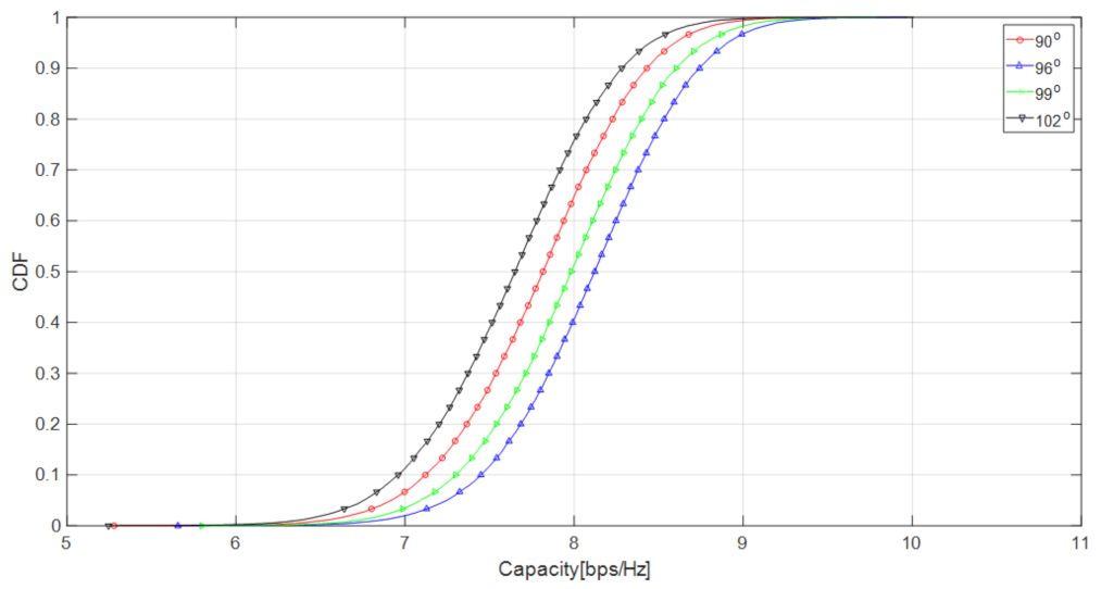
| Line-of-Sight Axis Elevation ) | 95.37° (Distance: 250 m) |
| Antenna Downtilt Angle ) | 90° 96° 99° 102° |
| Parameter | Value |
|---|---|
| Base Station (BS) Height (m) | 25 |
| Mobile Station (MS) Height (m) | 1.5 |
| Distance (m) | 100, 150, 200, 250 |
| Carrier Frequency | 2.65 GHz |
| Transmission Power | 20 dBm |
| Bandwidth | 20 MHz |
| Noise Power | −174 dBm/Hz |
| Number of Base Station (BS) Transmitting Antenna | 20 |
| Number of Mobile Station (MS) Receiving Antenna | 1 |
| Number of Paths | 40 |
| Path Attenuation | |
| Vertical Half Beam Width ) | 15° |
| Horizontal Half Beam Width ) | 70° |
| Emission Angle Spread ) | 7° |
| Incidence Angle Spread ) | 10° |
| Transmitting Path Divergence Degree ) | 5 |
| Receiving Path Divergence Degree () | 5 |
| Line-of-Sight Axis Elevation () | 103.2246° (Distance: 100 m) 98.9040° (Distance: 150 m) 96.7015° (Distance: 200 m) 95.3700° (Distance: 250 m) |
| Antenna Downtilt Angle ) | for ideal condition 90°–125° for adaptive adjustment |
| Parameter | Value |
|---|---|
| Base Station (BS) Height (m) | 25 |
| Mobile Station (MS) Height (m) | 1.5 |
| Distance (m) | 100, 150, 200, 250 |
| Carrier Frequency | 2.65 GHz |
| Transmission Power | 20 dBm |
| Bandwidth | 20 MHz |
| Noise Power | −174 dBm/Hz |
| Number of Base Station (BS) Transmitting Antenna | 60 |
| Number of Mobile Station (MS) Receiving Antenna | 4 |
| Number of Paths | 40 |
| Path Attenuation | |
| Vertical Half Beam width () | 15° |
| Horizontal Half Beam Width () | 70° |
| Emission Angle Spread () | 7° |
| Incidence Angle Spread () | 10° |
| Transmitting Path Divergence Degree () | 5 |
| Receiving Path Divergence Degree () | 5 |
| Line-of-Sight Axis Elevation () | 103.2246° (Distance: 100 m) 98.9040° (Distance: 150 m) 96.7015° (Distance: 200 m) 95.3700° (Distance: 250 m) |
| Antenna Downtilt Angle () | for ideal condition 90°–125° for adaptive adjustment |
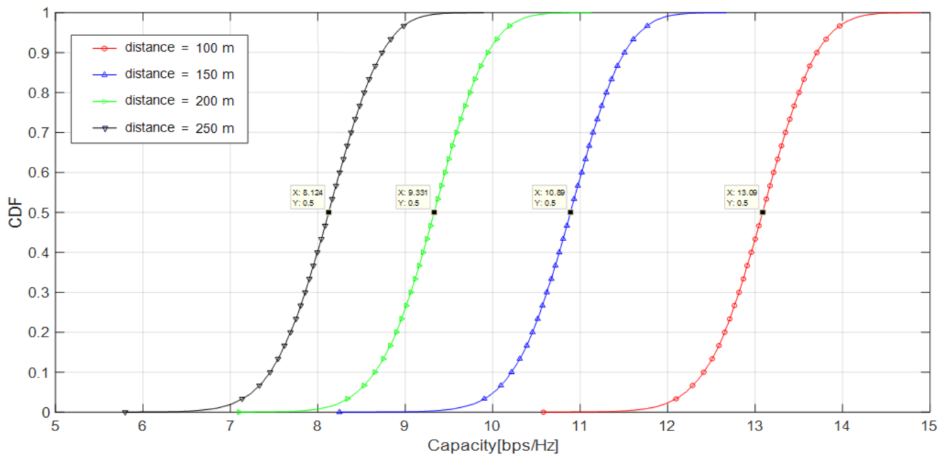
| Distance (m) | Receiver SNR | Channel Capacity |
|---|---|---|
| 100 | 39.6 dB | 13.09 bps/Hz |
| 150 | 33 dB | 10.89 bps/Hz |
| 200 | 28.3 dB | 9.331 bps/Hz |
| 250 | 24.6 dB | 8.124 bps/Hz |
| Distance (m) | Receiver SNR | Channel Capacity |
|---|---|---|
| 100 | 157.6 dB | 51.80 bps/Hz |
| 150 | 131 dB | 43.03 bps/Hz |
| 200 | 112.3 dB | 36.78 bps/Hz |
| 250 | 7.8 dB | 31.95 bps/Hz |
| Optimization Angle | Error Rate | Optimized Capacity | Capacity Efficiency | |
|---|---|---|---|---|
| 0.9 | 103° | 0.22% | 13.08 bps/Hz | 99.92% |
| 0.5 | 115.5° | 11.89% | 11.51 bps/Hz | 87.93% |
| 0.1 | 119.5° | 16.77% | 10.45 bps/Hz | 79.83% |
| Optimization Angle | Error Rate | Optimized Capacity | Capacity Efficiency | |
|---|---|---|---|---|
| 0.9 | 99° | 0.10% | 10.89 bps/Hz | 100% |
| 0.5 | 104.5° | 5.66% | 10.53 bps/Hz | 96.69% |
| 0.1 | 116.5° | 17.79% | 7.86bps/Hz | 72.18% |
| Optimization Angle | Error Rate | Optimized Capacity | Capacity Efficiency | |
|---|---|---|---|---|
| 0.9 | 97° | 0.31% | 9.313 bps/Hz | 99.81% |
| 0.5 | 103° | 6.51% | 8.883bps/Hz | 95.2% |
| 0.1 | 92° | 4.86% | 9.064 bps/Hz | 97.14% |
| Optimization Angle | Error Rate | Optimized Capacity | Capacity Efficiency | |
|---|---|---|---|---|
| 0.9 | 95° | 0.39% | 8.109 bps/Hz | 99.82% |
| 0.5 | 91° | 4.58% | 7.885 bps/Hz | 97.06% |
| 0.1 | 107° | 4.86% | 6.702 bps/Hz | 82.50% |
| Optimization Angle | Error Rate | Optimized Capacity | Capacity Efficiency | |
|---|---|---|---|---|
| 0.9 | 103° | 0.22% | 51.75 bps/Hz | 99.90% |
| 0.5 | 115.5° | 11.89% | 45.25 bps/Hz | 87.36% |
| 0.1 | 119° | 15.23% | 41.25 bps/Hz | 79.63% |
| Optimization Angle | Error Rate | Optimized Capacity | Capacity Efficiency | |
|---|---|---|---|---|
| 0.9 | 99° | 0.90% | 42.95 bps/Hz | 99.81% |
| 0.5 | 104.5° | 4.60% | 41.51 bps/Hz | 96.47% |
| 0.1 | 119° | 19.11% | 27.23 bps/Hz | 63.28% |
| Optimization Angle | Error Rate | Optimized Capacity | Capacity Efficiency | |
|---|---|---|---|---|
| 0.9 | 97° | 0.31% | 36.71 bps/Hz | 99.81% |
| 0.5 | 105° | 8.58% | 33.69 bps/Hz | 91.60% |
| 0.1 | 112° | 15.82% | 26.84 bps/Hz | 72.97% |
| Optimization Angle | Error Rate | Optimized Capacity | Capacity Efficiency | |
|---|---|---|---|---|
| 0.9 | 96° | 0.66% | 31.87 bps/Hz | 99.75% |
| 0.5 | 93.5° | 1.96% | 31.73 bps/Hz | 99.37% |
| 0.1 | 111.5° | 16.91% | 21.11 bps/Hz | 66.07% |
Publisher’s Note: MDPI stays neutral with regard to jurisdictional claims in published maps and institutional affiliations. |
© 2022 by the authors. Licensee MDPI, Basel, Switzerland. This article is an open access article distributed under the terms and conditions of the Creative Commons Attribution (CC BY) license (https://creativecommons.org/licenses/by/4.0/).
Share and Cite
Lee, S.-H.; Shi, X.-P.; Tan, T.-H.; Tung, Y.-C.; Huang, Y.-F. Maximizing Channel Capacity of 3D MIMO System via Antenna Downtilt Angle Adaptation Using a Q-Learning Algorithm. Electronics 2022, 11, 1189. https://doi.org/10.3390/electronics11081189
Lee S-H, Shi X-P, Tan T-H, Tung Y-C, Huang Y-F. Maximizing Channel Capacity of 3D MIMO System via Antenna Downtilt Angle Adaptation Using a Q-Learning Algorithm. Electronics. 2022; 11(8):1189. https://doi.org/10.3390/electronics11081189
Chicago/Turabian StyleLee, Shu-Hung, Xiao-Pei Shi, Tan-Hsu Tan, Yu-Che Tung, and Yung-Fa Huang. 2022. "Maximizing Channel Capacity of 3D MIMO System via Antenna Downtilt Angle Adaptation Using a Q-Learning Algorithm" Electronics 11, no. 8: 1189. https://doi.org/10.3390/electronics11081189
APA StyleLee, S.-H., Shi, X.-P., Tan, T.-H., Tung, Y.-C., & Huang, Y.-F. (2022). Maximizing Channel Capacity of 3D MIMO System via Antenna Downtilt Angle Adaptation Using a Q-Learning Algorithm. Electronics, 11(8), 1189. https://doi.org/10.3390/electronics11081189