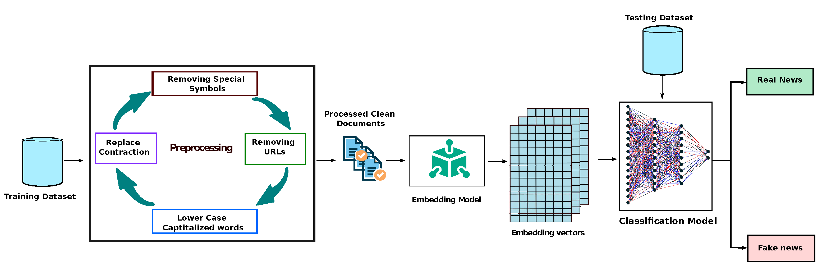
3.2. Word Embedding
Word embedding is a methodology that is used to transform textual data (words) into vectors. The main concept behind the word embedding is that words that are similar to each other will be close in the dimension space. Consequently, each word is characterized through an n-dimensional dense vector. Unlike other embedding methods like Word2vec, GloVe obtains word vectors by including global data (word co-occurrence).
We adopted the GloVe model (Global Vectors) in our model since it was created to examine the local context and global statistics of words before embedding them. The GloVe model’s central notion is that it emphasizes the co-occurrence probabilities of words within a corpus of texts in order to embed them in meaningful vectors, as indicated in Equation (
2). In other words, we are interested in the frequency with which a word
j occurs in the context of a word
i across our corpus of texts.
where
X is a word-word co-occurrence matrix,
is the frequency that word
j emerges in the context of word
i.
The GloVe model’s objective is to construct a function
F that can predict such ratios given two-word vectors word
i and word
j and a context word vector for word
k as parameters, as shown in Equation (
3).
Subsequently, GloVe will demonstrate the appropriate word vectors
and
throughout the training in order to reduce this weighted least squares issue. Furthermore, a weight function
must be employed to limit the significance of very frequent co-occurrences (such as “this is”) and to avoid uncommon co-occurrences from having the same significance as common ones.
In conclusion, the GloVe model takes advantage of a relevant source of information to fulfill the requested word resemblance task: co-occurrence probability ratios. Following that, it constructs an objective function J that maps word vectors to text statistics. Finally, GloVe minimizes the J function by learning incentive for word vectors.
Accordingly, to generate the embedding matrix for all words, we relied on the Golve embedding [
29]. The Golve is an unsupervised learning approach that creates representations for words in the form of vectors. The resultant representations emphasized fascinating linear substructures of the word vector space, which are trained using aggregated global word-word co-occurrence information extracted from a corpus. In our model, we used glove.840B.300d, which has a 300-dimensional vector embedding.
3.3. Classification Model
In the classification model, we implemented three experiments. In the first experiment, we applied machine learning algorithms, such as support vector machine (SVM), random forest (RF), and decision tree (DT). In the second experiment, we experimented with our dataset with long short-term memory (LSTM) and gated recurrent units (GRU) models. These models are considered the most popular deep learning models that deal with sequences. However, in the third experiment, we experimented with the BERT transformer to predict fake news.
LSTM and GRU are methodologies for deep learning that rely on recurrent neural networks (RNNs). Due to the ineffectiveness of RNN for long-term learning, LSTM and GRU were developed. GRU may also be regarded as a variant of the LSTM, since both are constructed similarly and give similar outstanding outcomes in certain circumstances. Using the LSTM or GRU architecture, any long-term interdependence may be retained and taught at random intervals. Additionally, LSTM or GRU are not dependent on any vectorization method, like
tfidf [
30].
LSTM outperformed RNN by including a module called constant error carousel (CEC). CEC spreads constant error signals across time, leveraging a well-designed “gate” structure to prevent backpropagated faults from fading or rising. As it switches to control data flow and memory, the “gate” structure calculates the internal value of CEC depending on the current input values and previous context.
Therefore, for any given sequence of words,
, the input gate, forget gate, and output gate in the LSTM structure, are notated as
,
, and
, respectively. The weight and bias values associated to the above gates are
,
,
,
,
,
, respectively. Through every step, LSTM updates two states: the hidden state
, and the cell state
, and
denotes the sigmoid function. The above parameters are presented as follows:
GRU was intended to address the long-short dependence issue with disappearing and inflating gradients, which is another well-known use of LSTM [
31]. Accordingly, GRU is purpose-built to work with sequential data that exhibits patterns across time steps, such as time-series data. The construction of GRU is more simpler than that of LSTM, which comprises three gates: an input gate, a forget gate, and an output gate. As a result, the training speed of GRU is somewhat quicker than that of the LSTM.
The update gate specifies the amount of data that should be added to the next state cell. When the update gate value is greater, more information is sent to the next state cell. The reset gate specifies how much prior data should be erased.
Therefore, some information generated from the previous cell might be ignored or forgotten when the value of the reset gate evolves. Therefore, some information generated from the previous cell might be ignored or forgotten when the value of the reset gate is higher [
31]. The following equation describes the update gate
, and the reset gate
.
The hidden state associated with the specific time step t is calculated using a linear interpolation of the prior activation function at step and the candidate hidden state .
Both the concealed state and the prospective concealed state are defined as follows:
where
,
, and
denote the input weighted matrices. Moreover, the parameters
,
, and
are the recurrent weight matrices. The vectors
and
denote the bias vectors. Finally, the function
denotes the activation function.
Our model examines the possible stacking of LSTM layers or GRU layers. Therefore, we experimented with a single LSTM or GRU layer, double LSTM or GRU layers, and finally triple LSTM or GRU layers. During our first experiment, we set our LSTM or GRU models to have a number of neurons of 128. In our second experiment, we stack another LSTM/GRU layer with a number of neurons set to 64. Finally, in our third experiment, we stacked another LSTM/GRU layer with a number of neurons set to 32.
During our experimentation, we fit our task to be a binary classification. Accordingly, we trained our LSTM and GRU models to return zero for real news and one for fake news. We used the ADAM optimizer with an early stopping condition to avoid the training overfitting. In addition, we use a learning rate of 0.001 and a batch size of 64.
Recently, most natural language processing applications have employed the use of Transformers [
32]. Transformers is a two-part design that enables the transformation of one sequence into another (Encoder and Decoder). Nonetheless, it is distinct from the sequence-to-sequence mentioned in the above models in that it does not refer to recurrent networks (GRU, LSTM, etc.). The Bidirectional Encoder Representations from Transformers (BERT) is a Google-developed transformer-based machine learning approach for pre-training natural language processing (NLP) [
33,
34]. Unlike traditional directional models that scan incoming text input sequentially either (left-to-right or right-to-left), the Transformer encoder reads the full sequence of words simultaneously. This property enables the model to infer the context of a word from its surroundings (left and right of the word). As a result, it is classified as bidirectional. However, it is more proper to describe it as non-directional [
35,
36].


