Global Formulation of the Synthetic Storm Technique Oriented to Satellite Link–Budget Design

Abstract

We have updated the global Synthetic Storm Technique (referred to as the global SST) by reformulating it according to a larger database of rain rate time series collected in several sites in different climatic regions. For each site, the average annual probability distribution of rain attenuation obtained with the global SST, $P_{SST,glo}\left(A\right),$ in a slant path, was compared with that given by the full SST, $P_{SST}\left(A\right),$ which we have considered as experimental data. The test was performed for frequency ranging from 10 to 100 GHz, for elevation angle $\theta$ ranging from 20° to 60° and for annual probabilities 10% to 0.01%. The global SST tends to underestimate the attenuation by approximately $10\%$ for elevation angle $\theta \le 30°$ and about $20\%$ for $30°<\theta <60°$ in the probability range 10% to 0.1%, and approximately $15\%$ in the probability range 0.1% to 0.01%. For any probability, the error is zero for $\theta =90°$ because at the zenith, the global SST coincides with the full SST.

1. Introduction

Satellite communication links at centimeter and millimeter wave frequencies can be affected by large rain attenuation. For a reliable link budget design, we need to know the annual probability distribution function, $P\left(A\right),$ of rain attenuation $A$ (dB) measured/predicted in the up- or down-link to the satellite. Instead of long and expensive measurements of beacon attenuation, prediction models are used for estimating $P\left(A\right)$ from a locally measured or estimated annual probability distributions function, $P\left(R\right),$ of 1-min rain rate $R$. However, after more than 40 years of modeling experimental results, there is no consensus on which prediction model is the most accurate and reliable. The Synthetic Storm Technique (SST) [1] is a powerful and accurate tool, as is now recognized, that can produce all the necessary statistics of rain attenuation, not only $P\left(A\right)$, but also fade durations and rate of change of attenuation because it provides reliable rain attenuation time series $A\left(t\right)$ [2]. From knowing rain rate time series $R\left(t\right)$ (mm/h, averaged in 1 min intervals), recorded at a site, the SST can generate $A\left(t\right)$, at any frequency and polarization, and for any slant path above about 10°. Because it reproduces reliable $A\left(t\right)$, it has been used in the last 30 years for many purposes, by several researchers [3,4,5,6,7,8,9,10,11,12,13,14,15,16,17,18,19,20,21,22,23,24,25,26,27,28,29,30,31,32,33], as Table 1 summarizes.

Table 1. References and applications of the Synthetic Storm Technique (SST).

Reference, Year	SST Application
1996 [1]	Mathematical theory of the Synthetic Storm Technique (SST), with two vertical layers of precipitation: 0 °C (melting layer), 20 °C (rainfall)
2005 [2]	SST-derived $A\left(t\right)$ can substitute missing experimental data (Italsat).
1994 [3]	The power spectrum of experimental $A\left(t\right)$ falls off as $-20 \mathrm{dB}/\mathrm{dec}$ (anticipation of the SST theory).
1997 [4]	Fade durations.
1998 [5]	Satellite communications with mobile transmitters/receivers.
1998 [6]	Diurnal distribution of rain attenuation in communication and broadcasting satellite systems.
1998 [7]	Wide area joint probability of rain attenuation in satellite systems with a common on-board resource.
1998 [8]	Worst-month statistics of rain attenuation.
1999 [9]	Large distance site diversity.
2000 [10]	Matching service quality and system design to the time of the day.
2003 [11]	Small scale (“micro”) site diversity.
2003 [12]	Statistics of interruption time due to rain attenuation.
2004 [13]	Service oriented statistics of interruption time.
2006 [14]	Annual and diurnal satellite rain attenuation statistics in Athens.
2006 [15]	Low elevation angle (5°) terrestrial paths.
2006 [16]	Time diversity as a rain attenuation countermeasure.
2007 [17]	Rain storms speed and temporal properties of precipitation.
2007 [18]	Time diversity gain in satellite links.
2007 [19]	SST as part of a time series generator.
2008 [20]	Tropical attenuation statistics.
2009 [21]	Phase delay and attenuation in deep-space tracking.
2011 [22]	Phase delay and differential attenuation in phased array antennas for deep-space communications.
2013 [23]	Small scale site diversity in Guam.
2013 [24]	Efficiency of satellite channels and ideal fade-countermeasure.
2016 [25]	Space communications to the Sun–Earth Lagrangian point L1 from Spino d’Adda.
2016 [26]	Space communications to the Sun–Earth Lagrangian point L1 from Madrid.
2016 [27]	A method to achieve clear-sky data-volume download in satellite links affected by tropospheric attenuation.
2016 [28]	Rain Attenuation Statistics at Ka and Q band in Athens.
2017 [29]	Linear combining techniques using time diversity.
2018 [30]	Rain attenuation statistics for micro and millimeter wavelengths.
2018 [31]	Fade dynamics in equatorial Malaysia.
2019 [32]	Space diversity in Attica, Greece.
2021 [33]	Time series of rain attenuation in a tropical location.

However, 1-min rain rate time series $R\left(t\right)$ are seldom available at a site. At most, at satellite ground stations, only the $P\left(R\right)$ of 1-min $R$ might be available. When these on–site measurements are not available, the ITU-R worldwide model can be used [34], although now it is possible to estimate the $P\left(R\right)$ of 1-min $R$ from historical (long term) rainfall averaged in much longer intervals, up to 24 h [35,36]. Therefore, based on the full SST, the previous version of the global SST model was studied many years ago [37]. From locally measured/estimated $P\left(R\right)$ it calculates $P\left(A\right)$ in a slant path, according to a simple relationship and variable transformation. The relationship was derived by studying how the rain attenuation time series $A\left(t\right)$ calculated with the SST, in a slant path of precipitation path length L, is built up by partial values $\Delta A\left(t\right)$ in partial precipitation path lengths $\Delta L$ [38].

The purpose of this paper is to update the global SST according to the results obtained from a larger database of rain rate time series collected at several sites in different climatic regions than those used many years ago. For each site, the average annual probability distribution of rain attenuation obtained with the global SST, $P_{SST,glo}\left(A\right),$ is compared with that given by the full SST, $P_{SST}\left(A\right),$ which we consider as experimental data. The test is conducted for frequencies ranging from 10 to 100 GHz, for elevation angle $\theta$ ranging from 20° to 90°, and for all annual probabilities 10% to 0.01%.

Finally, we recommend that whenever 1-min rain rate time series $R\left(t\right)$ are available at a site the full SST [1] be used.

After this Introduction, Section 2 describes the full SST and the global SST, Section 3 models the fundamental parameter $m$ of the global SST, Section 4 reports the results of the comparison between the full SST and the global SST, Section 5 reports the overall error and a discussion on the results. Finally, Section 6 draws some conclusions. In Appendix A, we show the scatter plots of the error for each site considered.

2. The Full SST and the Global SST

In this section we first sketch a brief summary of the theory of the full SST [1] and then recall the global SST [37,38].

2.1. The Full SST

A synthetic storm is obtained by converting a rain rate time series $R\left(t\right)$, recorded at a site by a rain gauge and averaged over 1 min, to a rain rate space series $R\left(x\right)$ along a line ($x-\mathrm{axis})$, by using an estimate of the storm translation speed $v$ to transform time to distance. Then, the specific rain attenuation $Y\left(x,t\right)$ (dB/km), calculated from the rain rate time series, is integrated along the path to obtain the rain attenuation time series $A_{SST}\left(t\right)$. The mathematical operation to obtain $A_{SST}\left(t\right)$ is a convolution from which, through Fourier transforms, useful theorems and conservation properties have been derived [1].

The SST can generate rain attenuation time series at any frequency and polarization, and for any slant path above about $10°$, as long as the hypothesis of isotropy of the rainfall spatial field holds, in the long term. The statistical properties of rain attenuation derived from a large sample of rain rate time series closely agree with those of the actual measured rain attenuation, and the predictions are significantly insensitive to a very precise value of $v$. If the motion of the rain storm is along the satellite path, then the measured $A\left(t\right)$ practically coincides with $A_{SST}\left(t\right)$, as shown for the ITALSAT experiment [39].

Rain attenuation time series can be simulated by using the value of v obtainable from measurements of wind speed, e.g., at 700 mbar height, extracted from the database of the European Centre for Medium-Range Weather Forecast [40]. The average horizontal rain–storm speed at Spino d’Adda is about 10.6 m/s, estimated directly from a meteorological radar [1], and in 1 min the rain storm moves a linear distance of 636 m.

The vertical (zenith) structure of precipitation is modelled with two layers of precipitation of different depths, a model taken from [41]. Starting from the ground there is rain (hydrometeors in the form of raindrops, water temperature of $20 °\mathrm{C}$, called layer A), followed by a melting layer, i.e., melting hydrometeors at $0 °\mathrm{C}$, layer B. The vertical rain rate R (mm/h) in layer A is assumed to be uniform and given by that measured at the ground, i.e., by the rain gauge, $R_A=R$. By assuming simple physical hypotheses, calculations show that the vertical precipitation rate in the melting layer, termed “apparent rain rate”, can also be supposed to be uniform and given by $R_B=3.134\times R_A$ [41]. The height of the precipitation (rain and melting layer, $H_R$) above sea level to be used in the simulation is the latest estimate of the ITU-R [42]. The layer B depth is 0.40 km, regardless of the latitude [41].

Let $H_S$ be the altitude of the site, $\theta$ be the elevation angle of the slant path, then the precipitation path length $L$ (km) is given by

$$L=\frac{H_R-H_S}{\sin \theta }=\frac{H_R-0.4-H_S}{\sin \theta }+\frac{0.4}{\sin \theta }=L_A+L_B$$

(1)

For example, at Spino d’Adda ($H_S=0.084$ km), $H_R=3.341$ km (see Table 2), therefore the length of the rainy path is $L=L_A+L_B=8.353+1.170=9.523$ km at $\theta =20°$, $L=5.714+0.800=6.514$ km at $\theta =30°$, $L=3.299+0.462=3.761$ km at $\theta =60°$, and, of course, $L=\left[\left(3.341-0.084\right)-0.4\right]+0.4=L_A+L_B=2.857+0.4=3257$ km at $\theta =90°$. In the zenith path ($\theta =90°)$, the rain rate is uniform, see Equation (29) of [1].

Table 2. Geographical coordinates, altitude (m), rain height $H_R$ (km) [42], number of years $n_Y$ of continuous rain rate measurements and wind speed $v$ (m/s) at 700 mbar altitude [40], except for Spino d’Adda whose rain storm speed was estimated from radar measurements [1].

Site	Lat. N (°)	Long. E (°)	Altitude ${\mathit{H}}_{\mathit{S}}$ (m)	Precipitation Height ${\mathit{H}}_{\mathit{R}}$ (km)	Years of Rain Rate Measurements ${\mathit{n}}_{\mathit{Y}}$	Wind Speed at 700 Mbar $\mathit{v}$ (m/s)
Spino d’Adda (Italy)	45.4	9.5	84	3.341	8	10.6
Gera Lario (Italy)	46.2	9.4	210	3.483	5	8.2
Fucino (Italy)	42.0	13.6	680	2.905	5	10.4
Madrid (Spain)	40.4	356.3	630	3.001	8	10.9
Prague (Czech Republic)	50.0	14.5	250	3.051	5	12.6
Tampa (Florida)	28.1	277.6	50	4.528	4	9.6
Norman (Oklahoma)	35.2	262.6	420	4.145	4	12.4
White Sands (New Mexico)	32.5	253.4	1463	4.744	5	9.1
Vancouver (British Columbia)	49.3	236.8	80	2.612	1	8.9
Fairbanks (Alaska)	64.9	212.2	184	2.688	3	12.4

2.2. The Global SST

Let us recall the first version of the global SST. In [37], we found that the $P_{SST}\left(A\right)$ generated by the SST can be approximately reproduced by calculating rain attenuation as

$$A=\left[C_o{k}_A{R}^{{\alpha }_A}+\left(1-C_o\right)k_B{\left(3.134\times R\right)}^{{\alpha }_B}\right]L^m$$

(2)

where $k$ and $\alpha$ are the constants that give the specific rain attenuation in the two layers from the rain rate R measured at the ground, calculated at $20 °\mathrm{C}$ in layer A and at $0 °\mathrm{C}$ in layer B [1]; values obtained from [43]. The constant $C_o$ is given by

$$C_o=\frac{L_A}{L}$$

(3)

For example, at Spino d’Adda $C_o=0.877$ at $\theta =20°$, therefore, a fraction $0.877$ of the attenuation is given by layer A and a fraction $1-C_o=0.123$ by layer B. Finally, notice that $L$ is not an equivalent path length because it does not depend on radio electrical parameters but it is calculated from Equation (1). The parameter $m$ is referred to as the average exponent of the global SST.

Now, by knowing the annual probability exceeded by R, $P\left(R\right),$ from (2) we can calculate the rain attenuation exceeded with the same probability and, therefore, $P\left(A\right)$, because of the simple transformation of the variable.

Of course, there are significant differences between $P_{SST}\left(A\right),$ obtained with the full SST, and $P_{SST,glo}\left(A\right)$, obtained from Equation (2), as shown in the previous version of the global SST [37]. In particular, the value $P_{SST,glo}\left(A>0\right)=P(R>0)$, is smaller than that calculated with the full SST, i.e., $P_{SST}\left(A>0\right)>P_{SST,glo}\left(A>0\right),$ because of the physical relationship described by Equation (18) of [1].

The aim of this paper is to estimate more reliable and global values of the exponent $m$ as a function of the elevation angle (in 5° steps) and frequency (in 5 GHz steps). Our actual estimates refer to the sites listed in Table 2, for which we have calculated the average value of $m$ and modelled it as reported in the next section.

3. Model of the Average Exponent of the Global SST

Following the observations and calculations reported in [37,38], and based on the rain attenuation time series $A_{SST}\left(t\right)$ obtained from the rain rate time series of the database recorded at the sites listed in Table 2, we have derived the following model of the average value of the parameter $m$, approximately valid in the range $20°\le \theta \le 90°$ and in the range $10\le f\le 100$ GHz. In the following, we have further distinguished three ranges of the elevation angle. The base of the logarithm is 10, the angle is in degrees, and frequency is in GHz.

Range (a): $70°\le \theta \le 90°$, $m=1$. No other action is required.

Range (b): $30<\theta <70°$.

• Calculate the value at 10 GHz, $m_{f10}\left(\theta \right)$

  $$m_{f10}\left(\theta \right)=2.34\times {10}^{-4}{\theta }^2-2.21\times {10}^{-2}\theta +1.38$$

  (4)
• Calculate the value at 100 GHz $m_{f100}\left(\theta \right)$

  $$m_{f100}\left(\theta \right)=1.22\times {10}^{-4}{\theta }^2-1.15\times {10}^{-2}\theta +1.2$$

  (5)
• Calculate the normalized average value $m_n\left(f\right)$ see Figure 1

  $$m_n\left(f\right)=-7.07\times {\left(\log f\right)}^4+44.73\times {\left(\log f\right)}^2-104.57\times {\left(\log f\right)}^2+107.69\times \log f-40.77$$

  (6)
• Calculate, finally, the denormalized value $m\left(f,\theta \right)$ to use in Equation (2)

  $$m\left(f,\theta \right)=m_n\left(f\right)\left[m_{f100}\left(\theta \right)-m_{f10}\left(\theta \right)\right]+m_{f10}\left(\theta \right)$$

  (7)

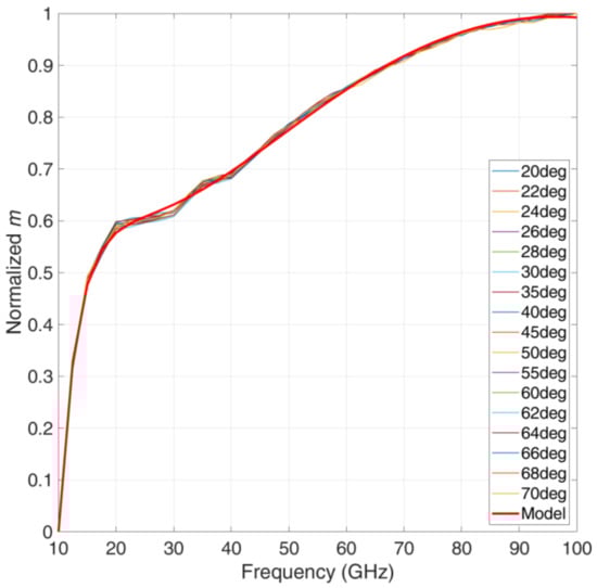Figure 1. Normalized value of the $\mathrm{average} \mathrm{exponent} \mathrm{of} \mathrm{the} \mathrm{global} \mathrm{SST}$, between 10 GHz and 100 GHz. The thin lines give the average value for each elevation angle. The thick red line gives the model $m_n\left(f\right)$. Notice that the normalized value of each elevation angle is practically the same, regardless of frequency and locality, a fundamental result that allows the modelling reported in step (3) of range (b). The superposition of the thin colored lines indicates that the global SST model can be applied to every site.

Range (c): $20°\le \theta <30°$.

• Calculate the probability (%)

  $$p=\left[0.1+0.005\times \left(f-20\right)\right]$$

  (8)
  This probability ranges between $p=0.1$ at $f=20$ GHz, and $p=0.5$ at $f=100$ GHz.
• For $p\le \left[0.1+0.005\times \left(f-20\right)\right]$, calculate $m\left(f,\theta \right)$

  $$m\left(f,\theta \right)=d_2{\left[\log \left(p\right)\right]}^2+d_1\log \left(p\right)+d_0$$

  (9)

  with

  $$d_2=\frac{m_1\times \log \left(0.8\right)+0.99\times \left(b+2\right)-2-a}{4\times \log \left(0.8\right)+2\left(a^2-b^2\right)+a^{2}b-a{b}^2}$$

  $$d_1=\frac{m_1\left(b^2-a^2\right)+0.99\times \left(4-b^2\right)+a^2-4}{4\times \log \left(0.8\right)+2\left(a^2-b^2\right)+a^{2}b-a{b}^2}$$

  $$d_0=\frac{m_{1}ab\left(a-b\right)-1.98\times b\left(b+2\right)+4a+2a^2}{4\times \log \left(0.8\right)+2\left(a^2-b^2\right)+a^{2}b-a{b}^2}$$

  $$m_1=2.30\times \left(1.71\times {10}^{-3}f+8.46\times {10}^{-2}\right)\times \log \left(\theta \right)-9.11\times {10}^{-3}f+0.643$$

  $$a=\log \left\{0.8\times \left[0.1+0.005\times \left(f-20\right)\right] \right\}$$

  $$b=\log \left[0.1+0.005\times \left(f-20\right)\right]$$
• For $p>\left[0.1+0.005\times \left(f-20\right)\right]$, no correction is required.

4. Results

Because of its reliability, we assume $A_{SST}\left(t\right)$ as experimental, calculate its annual average probability $P_{SST}\left(A\right)$ and compare (test) to it the probability $P_{SST,glo}\left(A\right)$, calculated according to the modelling of Section 3. The test is explicitly conducted for the elevation angle in the range $20°\le \theta \le 60°$ (5° steps) and for the frequency (5° GHz steps) in the range $10\le f\le 100$ GHz (5 GHz steps). At the boundary between any two ranges modelled in Section 3, we suggest considering the average of the two limit values.

Figure 2 and Figure 3 show $P_{SST}\left(A\right)$ and $P_{SST,glo}\left(A\right)$ obtained at Spino d’Adda, for different elevation angles and frequencies (circular polarization in the following). We can see that the global SST tends to underestimate the full SST.

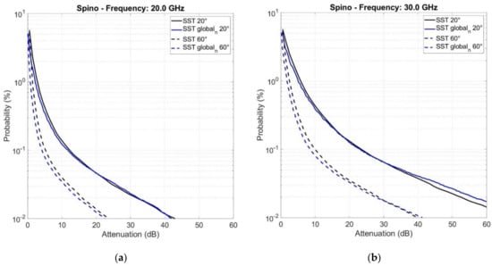
Figure 2. $P_{SST}\left(A\right)$ (black lines) and $P_{SST,glo}\left(A\right)$ (blue lines) at 20 GHz (a) and at 30 GHz (b) at Spino d’Adda, for $\theta =20°$ (continuous lines) and $\theta =60°$ (dashed lines).

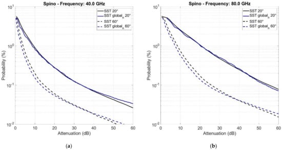
Figure 3. $P_{SST}\left(A\right)$ (black lines) and $P_{SST,glo}\left(A\right)$ (blue lines) at 40 GHz (a) and at 80 GHz (b) at Spino d’Adda, for $\theta =20°$ (continuous lines) and $\theta =60°$ (dashed lines).

We define a synthetic index of the test the error $\epsilon \left(\mathrm{dB}\right)$, defined at equal average annual probability $P$

$$\epsilon \left(P\right)=A_{SST,glo}\left(P\right)-A_{SST}\left(P\right)$$

(10)

The relative error is given by

$${\mathit{\epsilon }}_{\mathit{r}}\left(\mathit{P}\right)=\mathbf{100}\times \frac{{\mathit{A}}_{\mathit{S}\mathit{S}\mathit{T},\mathit{g}\mathit{l}\mathit{o}}\left(\mathit{P}\right)-{\mathit{A}}_{\mathit{S}\mathit{S}\mathit{T}}\left(\mathit{P}\right)}{{\mathit{A}}_{\mathit{S}\mathit{S}\mathit{T}}\left(\mathit{P}\right)}$$

(11)

For Spino d’Adda, Figure 4 shows the scatter plots of $\mathit{\epsilon }$, in the indicated range of elevation angles $\theta \le 30°$ and $\theta >30°$ without distinguishing frequency, probability and elevation angle. In Appendix A, we report the scatter plots for the other sites.

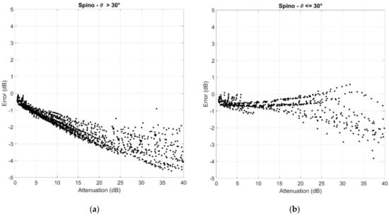
Figure 4. Scatter plots of the error $\epsilon =A_{SST,glo}-A_{SST}$ versus $A_{SST}$: (a) $\theta >30°$; (b) $\theta \le 30°$. Spino d’Adda.

In the next section we calculate and discuss the overall error.

5. Overall Error and Discussion

From the scatter plots shown in Figure 4 for Spino d’Adda and in Appendix A for the other sites, it is useful to calculate the average value and standard deviation of the error versus attenuation, in two disjoint ranges of probability, namely 10% to 0.1% and 0.1% to 0.01%, and in two disjoint ranges of elevation angle, $\theta \le 30°$ and $30<\theta \le 60°$, without distinguishing frequency, which plays a very minor role in error statistics, as the parameter $m$ depends very little on frequency (see the modelling in Section 3, or [38]).

These different ranges are useful because communication systems may be designed in the upper range (10% to 0.1%) instead of the more common lower range (0.1% to 0.01%), or with low elevation angles (in low satellite orbits, such as in LEO constellations). Our choice is due to the extremely large values of rain attenuation found at low probabilities or in low elevation angles, which would require, therefore, unavailable system power margins, if site diversity or other fade countermeasures are not used.

Figure 5 (probability range 10% to 0.1%) and Figure 6 (probability range 0.1% to 0.01%) show these statistics, calculated by considering all sites, in the range $0<A_{SST}\le 40$ dB, which should be a realistic range of tolerable attenuations and therefore power margins to provide to the link budget. From these results, we can derive the following conclusions.

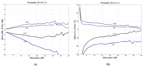
Figure 5. (a) Average (continuous lines) and standard deviation (dashed lines) of the error $\epsilon$ versus $A_{SST}$; (b) ${\epsilon }_r$. Probability range 10% to 0.1%.

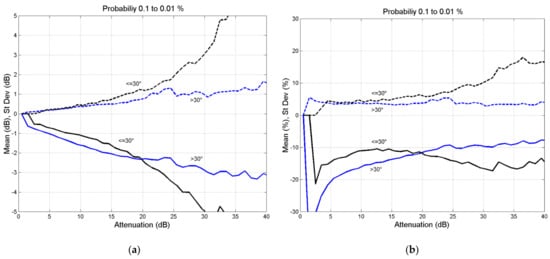
Figure 6. (a) Average (continuous lines) and standard deviation (dashed lines) of the error $\epsilon$ versus $A_{SST}$; (b) ${\epsilon }_r$. Probability range 0.1% to 0.01%.

In the probability range 10% to 0.1% (Figure 5):

• The error is always negative; in other words, the global SST tends to underestimate the attenuation.
• There is a significant difference between the elevation angle ranges, with the lower elevation angle range more accurate.
• The relative error is approximately $-10\%$ for $\theta \le 30°$ and about $-20\%$ for $\theta >30°$.
• The standard deviation is about 5% for both elevation angle ranges.

In the probability range 0.1% to 0.01% (Figure 5):

• The error is always negative; the global SST tends to underestimate the attenuation.
• There is not a significant difference between the two elevation angle ranges.
• The relative error is approximately $-15\%$.
• The standard deviation is about 5% for $\theta >30°$ and reaches 15% for $\theta \le 30°$.

Finally, notice that, for any probability, the error is negligible in the range $70°\le \theta <90°$ and it is zero for $\theta =90°$ because at the zenith, the global SST coincides with the full SST [1].

6. Conclusions

We have updated the global SST by reformulating it according to a larger database of rain rate time series collected in several sites in different climatic regions (Table 2). For each site, the average annual probability distribution of rain attenuation obtained with the global SST, $P_{SST,glo}\left(A\right),$ has been compared with that given by the full SST, $P_{SST}\left(A\right),$ which we have considered as experimental data. The test has been conducted for frequencies ranging from 10 to 100 GHz, for elevation angles $\theta$ ranging from 20° to 60° and for annual probabilities 10% to 0.01%.

To present the results oriented specifically to the link budget design, we have studied the probability ranges 10% to 0.1% and 0.1% to 0.01% separately because of the extremely large values of rain attenuation at high frequencies, which would require unavailable system power margins, if site diversity or other fade countermeasures are not used.

The global SST tends to underestimate the attenuation by approximately $10\%$ for elevation angle $\theta \le 30°$ and about $20\%$ for $30°<\theta <60°$ in the probability range 10% to 0.1%, and approximately $15\%$ in the probability range 0.1% to 0.01%.

For any probability, the error is zero for $\theta =90°$ because at the zenith the global SST coincides with the full SST.

References

- Matricciani, E. Physical–mathematical model of the dynamics of rain attenuation based on rain rate time series and a two–layer vertical structure of precipitation. Radio Sci. 1996, 31, 281–295. [Google Scholar] [CrossRef]
- Matricciani, E.; Riva, C. The search for the most reliable long–term rain attenuation cdf of a slant path and the impact on pre-diction models. IEEE Trans. Antennas Propag. 2005, 53, 3075–3079. [Google Scholar] [CrossRef]
- Matricciani, E. Physical–mathematical model of dynamics of rain attenuation with application to power spectrum. Electron. Lett. 1994, 30, 522–524. [Google Scholar] [CrossRef]
- Matricciani, E. Prediction of fade durations due to rain in satellite communication systems. Radio Sci. 1997, 32, 935–941. [Google Scholar] [CrossRef]
- Matricciani, E.; Moretti, S. Rain attenuation statistics useful for the design of mobile satellite communication systems. IEEE Trans. Veh. Technol. 1998, 47, 637–648. [Google Scholar] [CrossRef]
- Matricciani, E. Diurnal distribution of rain attenuation in communication and broadcasting satellite systems at 11.6 GHz in Italy. IEEE Trans. Broadcast. 1998, 44, 250–258. [Google Scholar] [CrossRef]
- Matricciani, E. Wide area joint probability of rain attenuation useful to design satellite systems with a common onboard resource: Experimental results obtained with the synthetic storm technique in Italy. In Proceedings of the Fourth Ka Band Utilization Conference, Venice, Italy, 2–4 November 1998; pp. 271–277. [Google Scholar]
- Matricciani, E. Worst–month statistics of rain attenuation in a satellite link at 19.77 GHz: Experimental results derived with the synthetic storm technique for the station of Gera Lario. In Proceedings of the Fourth Ka Band Utilization Conference, Venice, Italy, 2–4 November 1998; pp. 287–292. [Google Scholar]
- Matricciani, E.; Ordano, L.; Iorio, L. Large Distance Site Diversity in Satellite Communication Systems: Long Term Experimental Results obtained in Italy with the Synthetic Storm Technique. In Proceedings of the Fifth International Mobile Satellite Conference, Ottawa, ON, Canada, 16–18 June 1999; pp. 150–156. [Google Scholar]
- Matricciani, E. An assessment of rain attenuation impact on satellite communication: Matching service quality and system design to the time of the day. Space Commun. 2000, 16, 195–205. [Google Scholar]
- Matricciani, E. Micro Scale Site Diversity In satellite and Troposphere Communication Systems Affected By Rain Attenuation. Space Commun. 2003, 19, 83–90. [Google Scholar]
- Matricciani, E.; Riva, C. Statistics of Interruption Time Due to Rainfall in Satellite Communication Systems. In Proceedings of the 9th Ka Band Communications Conference, Ischia, Italy, 5–7 November 2003; pp. 207–214. [Google Scholar]
- Matricciani, E. Service Oriented Statistics of Interruption Time Due to Rainfall in Earth–Space Communication Systems. IEEE Trans. Antennas Propag. 2004, 52, 2083–2090. [Google Scholar] [CrossRef]
- Kanellopoulos, S.; Panagopoulos, A.; Matricciani, E.; Kanellopoulos, J. Annual and Diurnal Slant Path Rain Attenuation Statistics in Athens Obtained With the Synthetic Storm Technique. IEEE Trans. Antennas Propag. 2006, 54, 2357–2364. [Google Scholar] [CrossRef]
- Matricciani, E.; Riva, C.; Castanet, L. Performance of the Synthetic Storm Technique in a Low Elevation 5° Slant Path at 44.5 GHz in the French Pyrénées. In Proceedings of the EuCAP 2006, Nice, France, 6–10 November 2006. [Google Scholar]
- Matricciani, E. Time diversity as a rain attenuation countermeasure in satellite links in the 10–100 GHz frequency bands. In Proceedings of the EuCAP 2006, Nice, France, 6–10 November 2006; pp. 1–6. [Google Scholar] [CrossRef]
- Matricciani, E. Correlation between speed of rain storms and temporal properties of precipitation: Applications to the synthetic storm technique. In Proceedings of the EuCAP 2007, Edinburgh, UK, 11–16 November 2007. [Google Scholar] [CrossRef]
- Matricciani, E. Time diversity in satellite links affected by rain: Prediction of the gain at different localities. In Proceedings of the EuCAP 2007, Edinburgh, UK, 11–16 November 2007. [Google Scholar] [CrossRef]
- Sánchez-Lago, I.; Fontán, F.P.; Mariño, P.; Fiebig, U.C. Validation of the Synthetic Storm Technique as Part of a Time–Series Generator for Satellite Links. IEEE Antennas Wirel. Propag. Lett. 2007, 6, 372–375. [Google Scholar] [CrossRef]
- Mahmudah, H.; Wijayanti, A.; Mauludiyanto, A.; Hendrantoro, G.; Matsushima, A. Analysis of Tropical Attenuation Statistics using Synthetic Storm for Millimeter–Wave Wireless Network Design. In Proceedings of the 5th IFIP International Conference on Wireless and Optical Communications Networks (WOCN ’08), Surabaya, East Java, Indonesia, 5–7 May 2008. [Google Scholar]
- Matricciani, E. A Relationship between Phase Delay and Attenuation Due to Rain and Its Applications to Satellite and Deep-Space Tracking. IEEE Trans. Antennas Propag. 2009, 57, 3602–3611. [Google Scholar] [CrossRef]
- Matricciani, E. Phase delay and differential attenuation due to rain in large phased array antennas for deep-space communications at 32 GHz. In Proceedings of the EuCAP 2011, Rome, Italy, 11–15 April 2011; pp. 1–4. [Google Scholar]
- Acosta, R.; Matricciani, E.; Riva, C. Slant Path Attenuation and Microscale Site Diversity Gain Measured and Predicted in Guam with the Synthetic Storm Technique at 20.7 GHz. In Proceedings of the EuCAP 2013, Gothenburg, Sweden, 8–12 April 2013; pp. 1–4. [Google Scholar]
- Matricciani, E. Efficiency of Satellite Channels affected by Rain attenuation and Ideal Fade-Countermeasure Method. In Proceedings of the 20th Ka and Broadband Communications, Navigation and Earth Observation Conference, Florence, Italy, 14–17 October 2013. [Google Scholar]
- Matricciani, E. Space communications with variable elevation angle faded by rain: Radio links to the Sun–Earth first Lagrangian point L1. Int. J. Satell. Commun. Netw. 2016, 34, 809–831. [Google Scholar] [CrossRef][Green Version]
- Matricciani, E.; Riera, J.M. Variable elevation–angle radio links faded by rain at Ka Band from Madrid to the Sun–Earth La-grangian point L1. In Proceedings of the 22th Ka and Broadband Communications Conference, Cleveland, OH, USA, 17–20 October 2016. [Google Scholar]
- Matricciani, E. A method to achieve clear-sky data-volume download in satellite links affected by tropospheric attenuation. Int. J. Satell. Commun. Netw. 2016, 34, 713–723. [Google Scholar] [CrossRef]
- Lyras, N.K.; Kourogiorgas, C.I.; Panagopoulos, A.D.; Ventouras, S. Rain Attenuation Statistics at Ka and Q band in Athens using SST and Short Scale Dynamic Diversity Gain Evaluation. In Proceedings of the 2016 Loughborough Antennas & Propagation Conference (LAPC), Loughborough, UK, 14–15 November 2016. [Google Scholar]
- Matricciani, E. Probability distributions of rain attenuation obtainable with linear combining techniques in space-to-Earth links using time diversity. Int. J. Satell. Commun. Netw. 2017, 36, 220–237. [Google Scholar] [CrossRef]
- Nandi, A. Prediction of Rain Attenuation Statistics from Measured Rain Rate Statistics using Synthetic Storm Technique for Micro and Millimeter Wave Communication Systems. In Proceedings of the 2018 IEEE MTT–S International Microwave and RF Conference (IMaRC), Kolkata, India, 28–30 November 2018. [Google Scholar]
- Jong, S.L.; Riva, C.; D’Amico, M.; Lam, H.Y.; Yunus, M.M.; Din, J. Performance of synthetic storm technique in estimating fade dynamics in equatorial Malaysia. Int. J. Satell. Commun. Netw. 2018, 36, 416–426. [Google Scholar] [CrossRef]
- Papafragkakis, A.Z.; Kourogiorgas, C.I.; Panagopoulos, A.D. Performance Evaluation of Ka- and Q-band Earth–Space Diversity Systems in Attica, Greece using the Synthetic Storm Technique. In Proceedings of the 13th European Conference on Antennas and Propagation (EuCAP 2019), Krakow, Poland, 31 March–5 April 2019. [Google Scholar]
- Das, D.; Animesh Maitra, A. Application of Synthetic Storm Technique to Predict Time Series of Rain Attenuation from Rain Rate Measurement for a Tropical Location. In Proceedings of the 5th International Conference on Computers and Devices for Communication (CODEC), Kolkata, India, 17–19 December 2021. [Google Scholar]
- Recommendation ITU-R P.837-7. Characteristics of Precipitation for Propagation Modelling; ITU: Geneva, Switzerland, 2017. [Google Scholar]
- Matricciani, E. A mathematical theory of de-integrating long-time integrated rainfall and its application for predicting 1-min rain rate statistics. Int. J. Satell. Commun. Netw. 2011, 29, 501–530. [Google Scholar] [CrossRef]
- Matricciani, E. A mathematical theory of de–integrating long–time integrated rainfall statistics. Part II: From 1 day to 1 minute. Int. J. Satell. Commun. Netw. 2013, 31, 77–102. [Google Scholar] [CrossRef]
- Matricciani, E. Global formulation of the Synthetic Storm Technique to calculate rain attenuation only from rain rate probability distributions. In Proceedings of the 2008 IEEE International Symposium on Antennas and Propagation, San Diego, CA, USA, 5–11 July 2008. [Google Scholar] [CrossRef]
- Matricciani, E. A fundamental differential equation that links rain attenuation to the rain rate measured at one point, and its applications in slant paths. In Proceedings of the EuCAP 2006, Nice, France, 6–10 November 2006. [Google Scholar] [CrossRef]
- Matricciani, E.; Mauri, M.; Riva, C. A Rain Rate Data Base Useful to Simulate Reliable Rain Attenuation Time Series for Ap-plications to Satellite and Tropospheric Communication Systems. In Proceedings of the 2002 European Conference on Wireless Technology (ECWT 2002), Milan, Italy, 26–27 September 2002; pp. 265–268. [Google Scholar]
- ECMWF. Available online: https://www.ecmwf.int/en/forecasts/dataset/ecmwf-reanalysis-v5 (accessed on 28 March 2022).
- Matricciani, E. Rain attenuation predicted with a two-layer rain model. Eur. Trans. Telecommun. 1991, 2, 715–727. [Google Scholar] [CrossRef]
- Recommendation ITU-R P.839-4. Rain Height Model for Prediction Methods; ITU: Geneva, Switzerland, 2013. [Google Scholar]
- Maggiori, D. Computed transmission through rain in the 1–400 GHz frequency range for spherical and elliptical drops and any polarization. Alta Freq. 1981, 50, 262–273. [Google Scholar]
Publisher’s Note: MDPI stays neutral with regard to jurisdictional claims in published maps and institutional affiliations. |
© 2022 by the authors. Licensee MDPI, Basel, Switzerland. This article is an open access article distributed under the terms and conditions of the Creative Commons Attribution (CC BY) license (https://creativecommons.org/licenses/by/4.0/).