
Part-Aware Refinement Network for Occlusion Vehicle Detection


Abstract
:1. Introduction
- We propose a part-aware refinement network for occlusion vehicle detection, which optimizes the model with the component confidence strategy, and uses the confidence of the visible vehicle parts to correct the final detection confidence. Our proposed method can automatically extract the vehicle features, it has solved the problems of larger error when locating vehicles in traditional approaches, and improved the vehicle detection recall.
- we adopt the K-means clustering algorithm to generate a suitable anchor box size, adapt to the scale change of the dataset and improve the detection accuracy.
- we relabel the KITTI dataset, adding the detailed occlusion information of the vehicles. The new dataset can provide better supervision for occluded vehicle detection.
2. Proposed Method
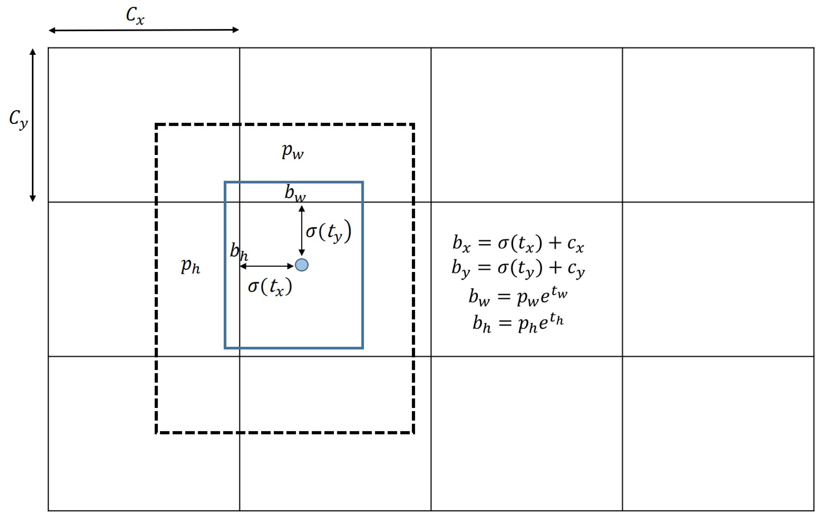
2.1. Preliminary Knowledge on Single-Stage Object Detection
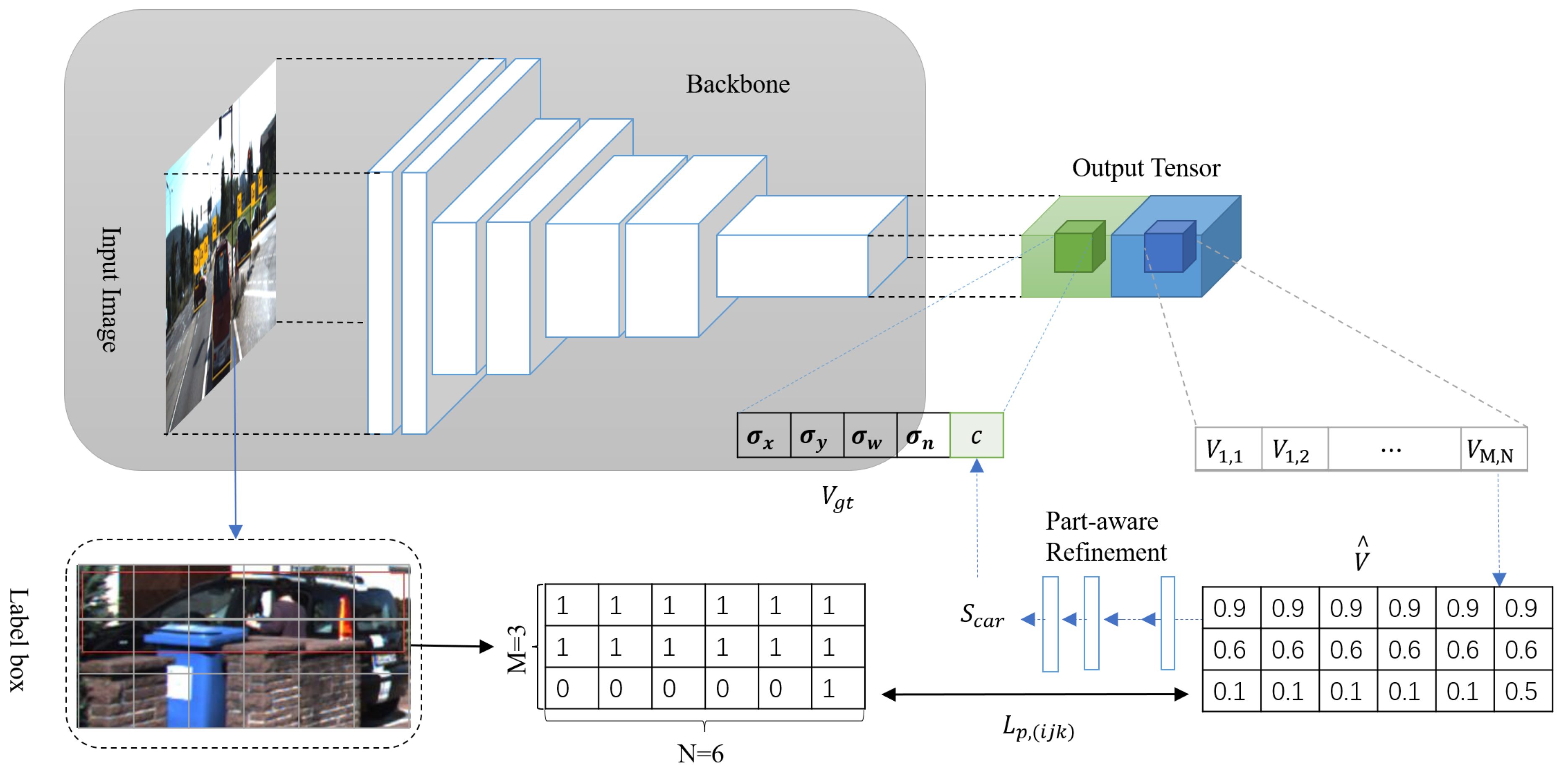
2.2. Part-Aware Refinement Network
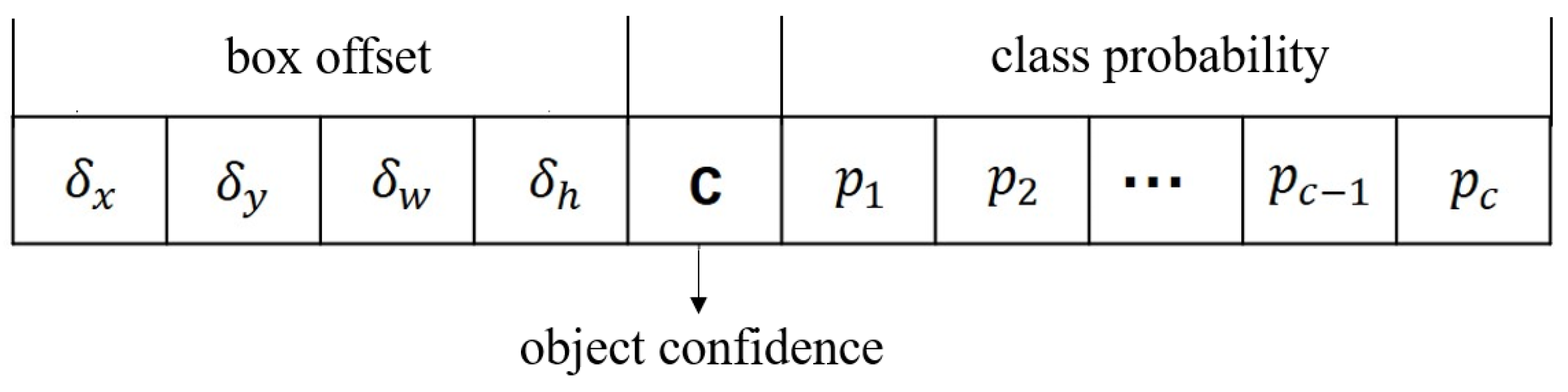
2.2.1. Output Tensor Overview
2.2.2. Part-Aware Refinement Network
2.2.3. Loss Function
3. Experimental Results
3.1. KITTI Dataset
3.2. Implementation Details
3.3. Multi-Scale Anchor Box Design
3.4. Ablation Studies
3.5. Compare the Detection Performance of the Two Algorithms in the Same Scene
3.6. Comparison with SOTA Methods
4. Conclusions
Author Contributions
Funding
Data Availability Statement
Acknowledgments
Conflicts of Interest
References
- Chang, L.; Chen, Y.T.; Wang, J.H.; Chang, Y.L. Modified YOLOv3 for Ship Detection with Visible and Infrared Images. Electronics 2022, 11, 739. [Google Scholar] [CrossRef]
- Jiang, X.; Gao, T.; Zhu, Z.; Zhao, Y. Real-time face mask detection method based on YOLOv3. Electronics 2021, 10, 837. [Google Scholar] [CrossRef]
- Liu, C.; Wu, Y.; Liu, J.; Sun, Z. Improved YOLOV3 network for insulator detection in aerial images with diverse background interference. Electronics 2021, 10, 771. [Google Scholar] [CrossRef]
- Wang, G.; Wang, Z.; Gu, K.; Jiang, K.; He, Z. Reference-free dibr-synthesized video quality metric in spatial and temporal domains. IEEE Trans. Circuits Syst. Video Technol. 2021, 32, 1119–1132. [Google Scholar] [CrossRef]
- Jiang, K.; Wang, Z.; Yi, P.; Chen, C.; Han, Z.; Lu, T.; Huang, B.; Jiang, J. Decomposition makes better rain removal: An improved attention-guided deraining network. IEEE Trans. Circuits Syst. Video Technol. 2020, 31, 3981–3995. [Google Scholar] [CrossRef]
- Jiang, K.; Wang, Z.; Yi, P.; Chen, C.; Wang, Z.; Wang, X.; Jiang, J.; Lin, C.W. Rain-free and residue hand-in-hand: A progressive coupled network for real-time image deraining. IEEE Trans. Image Process. 2021, 30, 7404–7418. [Google Scholar] [CrossRef]
- Jiang, K.; Wang, Z.; Yi, P.; Lu, T.; Jiang, J.; Xiong, Z. Dual-path deep fusion network for face image hallucination. IEEE Trans. Neural Netw. Learn. Syst. 2020, 33, 378–391. [Google Scholar] [CrossRef]
- Jiang, K.; Wang, Z.; Yi, P.; Wang, G.; Gu, K.; Jiang, J. ATMFN: Adaptive-threshold-based multi-model fusion network for compressed face hallucination. IEEE Trans. Multimed. 2019, 22, 2734–2747. [Google Scholar] [CrossRef]
- Wang, Z.; Jiang, J.; Yu, Y.; Satoh, S. Incremental re-identification by cross-direction and cross-ranking adaption. IEEE Trans. Multimed. 2019, 21, 2376–2386. [Google Scholar] [CrossRef]
- Wang, Z.; Jiang, J.; Wu, Y.; Ye, M.; Bai, X.; Satoh, S. Learning sparse and identity-preserved hidden attributes for person re-identification. IEEE Trans. Image Process. 2019, 29, 2013–2025. [Google Scholar] [CrossRef]
- Wang, Z.; Hu, R.; Chen, C.; Yu, Y.; Jiang, J.; Liang, C.; Satoh, S. Person reidentification via discrepancy matrix and matrix metric. IEEE Trans. Cybern. 2017, 48, 3006–3020. [Google Scholar] [CrossRef] [PubMed]
- Lienhart, R.; Maydt, J. An extended set of Haar-like features for rapid object detection. In Proceedings of the International Conference on Image Processing, Rochester, NY, USA, 22–25 September 2002; Volume 1, pp. 900–903. [Google Scholar]
- Negri, P.; Clady, X.; Hanif, S.M.; Prevost, L. A cascade of boosted generative and discriminative classifiers for vehicle detection. EURASIP J. Adv. Signal Process. 2008, 2008, 782432. [Google Scholar] [CrossRef] [Green Version]
- Ma, X.; Grimson, W.E.L. Edge-based rich representation for vehicle classification. In Proceedings of the Tenth IEEE International Conference on Computer Vision (ICCV’05) Volume 1, Beijing, China, 17–21 October 2005; Volume 2, pp. 1185–1192. [Google Scholar]
- Ahonen, T.; Hadid, A.; Pietikäinen, M. Face recognition with local binary patterns. In Proceedings of the European Conference on Computer Vision, Prague, Czech Republic, 11–14 May 2004; pp. 469–481. [Google Scholar]
- Teoh, S.S.; Bräunl, T. Symmetry-based monocular vehicle detection system. Mach. Vis. Appl. 2012, 23, 831–842. [Google Scholar] [CrossRef]
- Cao, X.; Wu, C.; Yan, P.; Li, X. Linear SVM classification using boosting HOG features for vehicle detection in low-altitude airborne videos. In Proceedings of the 2011 18th IEEE International Conference on Image Processing, Brussels, Belgium, 11–14 September 2011; pp. 2421–2424. [Google Scholar]
- Girshick, R.; Donahue, J.; Darrell, T.; Malik, J. Rich feature hierarchies for accurate object detection and semantic segmentation. In Proceedings of the IEEE Conference on Computer Vision and Pattern Recognition, Columbus, OH, USA, 23–28 June 2014; pp. 580–587. [Google Scholar]
- Girshick, R. Fast r-cnn. In Proceedings of the IEEE International Conference on Computer Vision, Santiago, Chile, 7–13 December 2015; pp. 1440–1448. [Google Scholar]
- Ren, S.; He, K.; Girshick, R.; Sun, J. Faster r-cnn: Towards real-time object detection with region proposal networks. In Proceedings of the Annual Conference on Neural Information Processing Systems 2015, Montreal, QC, USA, 7–12 December 2015; Volume 28. [Google Scholar]
- Uijlings, J.R.; Van De Sande, K.E.; Gevers, T.; Smeulders, A.W. Selective search for object recognition. Int. J. Comput. Vis. 2013, 104, 154–171. [Google Scholar] [CrossRef] [Green Version]
- Redmon, J.; Divvala, S.; Girshick, R.; Farhadi, A. You only look once: Unified, real-time object detection. In Proceedings of the IEEE Conference on Computer Vision and Pattern Recognition, Las Vegas, NV, USA, 27–30 June 2016; pp. 779–788. [Google Scholar]
- Redmon, J.; Farhadi, A. YOLO9000: Better, faster, stronger. In Proceedings of the IEEE Conference on Computer Vision and Pattern Recognition, Honolulu, HI, USA, 21–26 July 2017; pp. 7263–7271. [Google Scholar]
- Redmon, J.; Farhadi, A. YOLOv3: An incremental improvement. arXiv 2018, arXiv:1804.02767. [Google Scholar]
- Qiu, L.; Zhang, D.; Tian, Y.; Al-Nabhan, N. Deep learning-based algorithm for vehicle detection in intelligent transportation systems. J. Supercomput. 2021, 77, 11083–11098. [Google Scholar] [CrossRef]
- Luo, J.Q.; Fang, H.S.; Shao, F.M.; Zhong, Y.; Hua, X. Multi-scale traffic vehicle detection based on faster R–CNN with NAS optimization and feature enrichment. Def. Technol. 2021, 17, 1542–1554. [Google Scholar] [CrossRef]
- Li, Y.; Li, S.; Du, H.; Chen, L.; Zhang, D.; Li, Y. YOLO-ACN: Focusing on small target and occluded object detection. IEEE Access 2020, 8, 227288–227303. [Google Scholar] [CrossRef]
- Du, S.; Zhang, B.; Zhang, P.; Xiang, P.; Xue, H. FA-YOLO: An Improved YOLO Model for Infrared Occlusion Object Detection under Confusing Background. Wirel. Commun. Mob. Comput. 2021, 2021, 1896029. [Google Scholar] [CrossRef]
- Ryu, S.E.; Chung, K.Y. Detection Model of Occluded Object Based on YOLO Using Hard-Example Mining and Augmentation Policy Optimization. Appl. Sci. 2021, 11, 7093. [Google Scholar] [CrossRef]
- Neubeck, A.; Van Gool, L. Efficient non-maximum suppression. In Proceedings of the 18th International Conference on Pattern Recognition (ICPR’06), Hong Kong, China, 20–24 August 2006; Volume 3, pp. 850–855. [Google Scholar]
- Rosebrock, A. Intersection over Union (IoU) for Object Detection. Diambil Kembali Dari PYImageSearch. 2016. Available online: https://www.pyimagesearch.com/2016/11/07/intersection-over-union-iou-for-object-detection (accessed on 1 July 2021).
- Lin, T.Y.; Goyal, P.; Girshick, R.; He, K.; Dollár, P. Focal loss for dense object detection. In Proceedings of the IEEE International Conference on Computer Vision, Venice, Italy, 22–29 October 2017; pp. 2980–2988. [Google Scholar]
- Mathias, M.; Benenson, R.; Timofte, R.; Van Gool, L. Handling occlusions with franken-classifiers. In Proceedings of the IEEE International Conference on Computer Vision, Sydney, Australia, 1–8 December 2013; pp. 1505–1512. [Google Scholar]
- Tian, Y.; Luo, P.; Wang, X.; Tang, X. Deep learning strong parts for pedestrian detection. In Proceedings of the IEEE International Conference on Computer Vision, Santiago, Chile, 7–13 December 2015; pp. 1904–1912. [Google Scholar]
- Noh, J.; Lee, S.; Kim, B.; Kim, G. Improving occlusion and hard negative handling for single-stage pedestrian detectors. In Proceedings of the IEEE Conference on Computer Vision and Pattern Recognition, Salt Lake City, UT, USA, 18–23 June 2018; pp. 966–974. [Google Scholar]
- Fan, Q.; Brown, L.; Smith, J. A closer look at Faster R-CNN for vehicle detection. In Proceedings of the 2016 IEEE Intelligent Vehicles Symposium (IV), Gothenburg, Sweden, 19–22 June 2016; pp. 124–129. [Google Scholar]
- Liu, W.; Anguelov, D.; Erhan, D.; Szegedy, C.; Reed, S.; Fu, C.Y.; Berg, A.C. Ssd: Single shot multibox detector. In Proceedings of the European Conference on Computer Vision, Amsterdam, The Netherlands, 8–14 September 2016; pp. 21–37. [Google Scholar]
- Dai, J.; Li, Y.; He, K.; Sun, J. R-fcn: Object detection via region-based fully convolutional networks. In Proceedings of the Annual Conference on Neural Information Processing Systems 2016, Barcelona, Spain, 5–10 December 2016; Volume 29. [Google Scholar]
- Haritha, H.; Thangavel, S.K. A modified deep learning architecture for vehicle detection in traffic monitoring system. Int. J. Comput. Appl. 2021, 43, 968–977. [Google Scholar] [CrossRef]


| Model | Number of Anchors | Part-Aware Refinement | Recall (%) | Precision (%) |
|---|---|---|---|---|
| A | 9 | ✗ | 94.24 | 84.24 |
| B | 16 | ✗ | 94.56 | 85.42 |
| C | 9 | ✔ | 96.12 | 86.26 |
| D | 16 | ✔ | 97.09 | 87.52 |
| Method | Recall (%) | Precision (%) | Average IOU |
|---|---|---|---|
| Baseline | 94.24 | 84.64 | 72.38 |
| Ours | 97.09 | 87.52 | 78.03 |
| Method | SSD [37] | RFCN [38] | Faster R-CNN [20] | YOLOv3 [24] | FE-CNN [25] | RIAC [26] | MVD [39] | Ours |
|---|---|---|---|---|---|---|---|---|
| Precision (%) | 83.54 | 88.39 | 86.30 | 84.64 | 85.25 | 86.19 | 85.92 | 87.52 |
| Recall (%) | 94.93 | 97.62 | 96.34 | 94.24 | 94.87 | 96.55 | 96.14 | 97.09 |
| IOU | 74.39 | 76.11 | 75.99 | 74.26 | 72.38 | 76.11 | 75.96 | 78.03 |
| Time (s) | 0.177 | 0.281 | 0.293 | 0.082 | 0.083 | 0.151 | 0.097 | 0.091 |
Publisher’s Note: MDPI stays neutral with regard to jurisdictional claims in published maps and institutional affiliations. |
© 2022 by the authors. Licensee MDPI, Basel, Switzerland. This article is an open access article distributed under the terms and conditions of the Creative Commons Attribution (CC BY) license (https://creativecommons.org/licenses/by/4.0/).
Share and Cite
Wang, Q.; Xu, N.; Huang, B.; Wang, G. Part-Aware Refinement Network for Occlusion Vehicle Detection. Electronics 2022, 11, 1375. https://doi.org/10.3390/electronics11091375
Wang Q, Xu N, Huang B, Wang G. Part-Aware Refinement Network for Occlusion Vehicle Detection. Electronics. 2022; 11(9):1375. https://doi.org/10.3390/electronics11091375
Chicago/Turabian StyleWang, Qifan, Ning Xu, Baojin Huang, and Guangcheng Wang. 2022. "Part-Aware Refinement Network for Occlusion Vehicle Detection" Electronics 11, no. 9: 1375. https://doi.org/10.3390/electronics11091375
APA StyleWang, Q., Xu, N., Huang, B., & Wang, G. (2022). Part-Aware Refinement Network for Occlusion Vehicle Detection. Electronics, 11(9), 1375. https://doi.org/10.3390/electronics11091375