
A Variable-Weather-Parameter Optimization Strategy Based on an Irradiance and Temperature Estimation Method for PV System

Abstract
:1. Introduction
- (1)
- An equation set for estimating the real-time I&T values under changeless weather conditions is established. This work is the first attempt to obtain the real-time I&T values by equation solution at the MPP of the PV system.
- (2)
- Two equations for estimating the real-time irradiance values under varying weather conditions are proposed. This work is the first attempt to estimate the real-time irradiance by two established empirical formulas.
- (3)
- A VWP optimization strategy based on the estimated I&T values is proposed, and its control process is designed. This work is the first attempt to implement the VWP method by estimating the real-time values of the irradiance and temperature.
- (4)
- In this work, the external data or measured values of the irradiance and temperature are no longer needed to implement the existing VWP methods. Therefore, it is a major breakthrough in cutting the cost of sensors and promoting the use of these methods.
2. Estimation Method under Changeless Weather Conditions
2.1. Mathematical Model of PV System
2.2. Principle of the Parameter Estimation
3. Estimation Method under Varying Weather Conditions
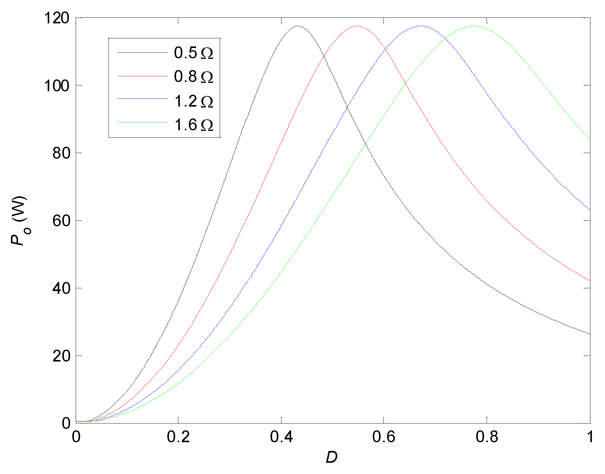
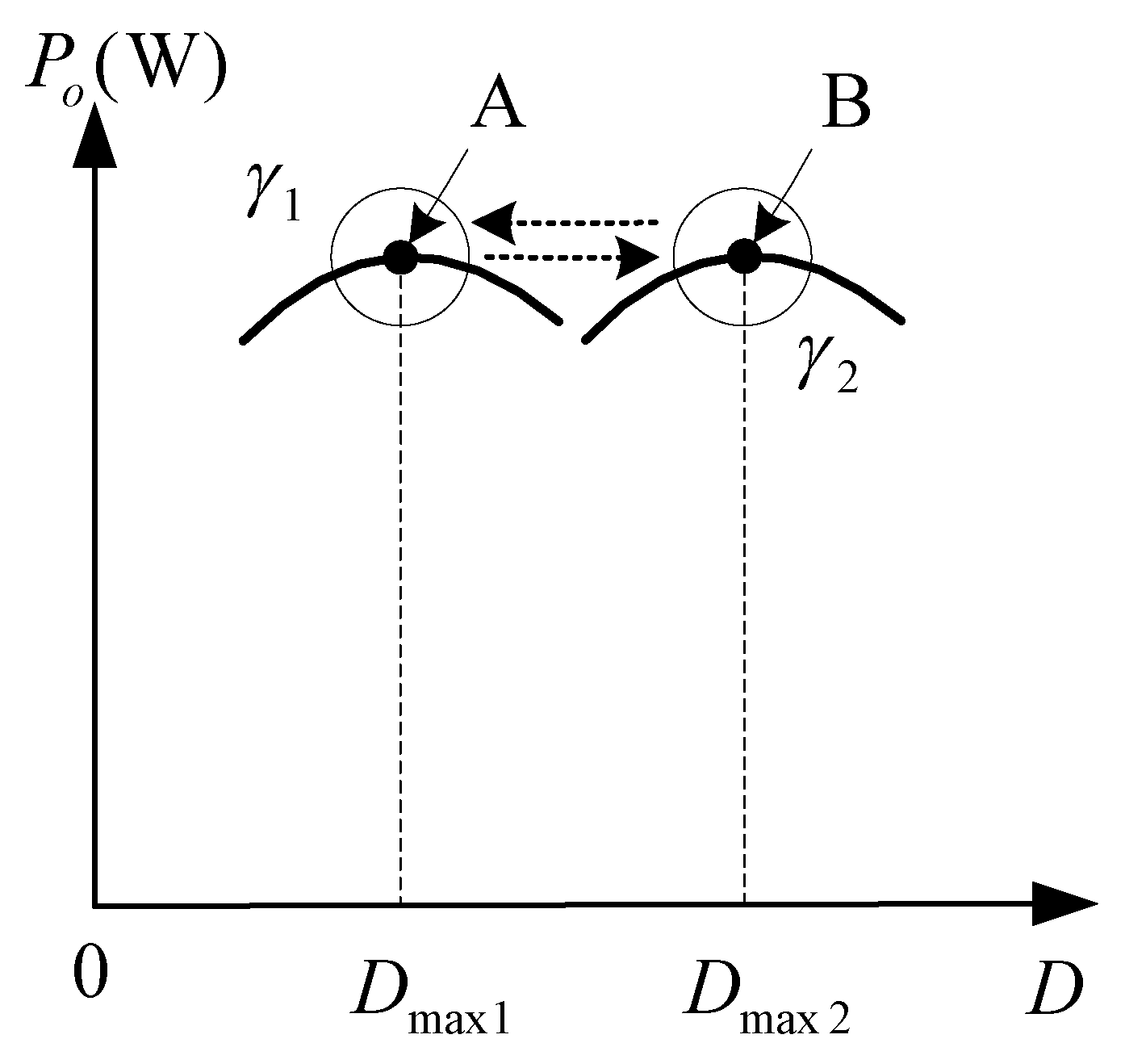
3.1. MPP Characteristics Changing with Weather Conditions
3.2. Proposed Equations for Estimating the Real-Time Irradiance
3.3. Estimation of the Real-Time Temperature
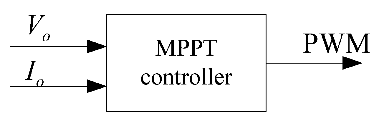
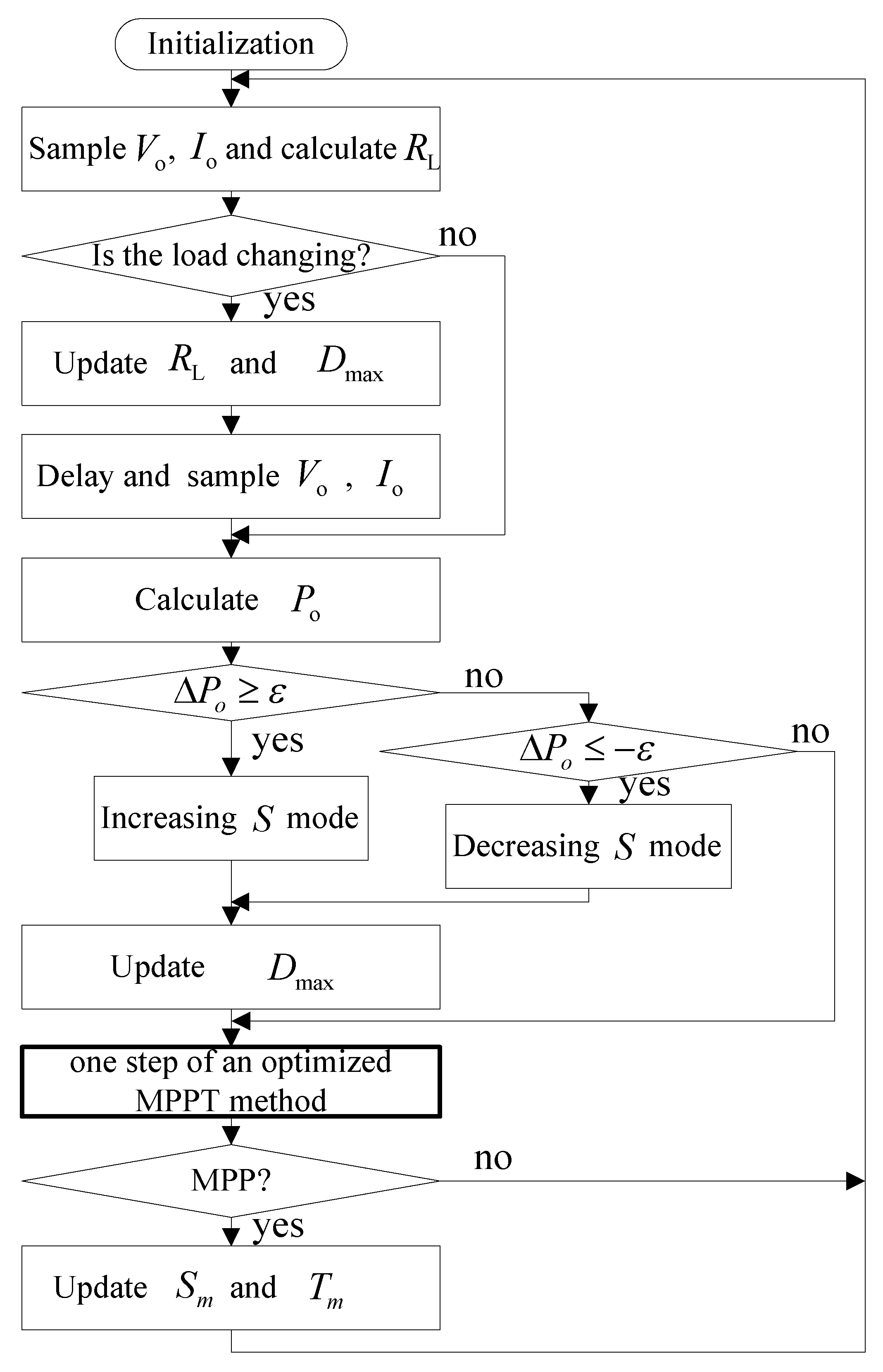
4. MPPT Optimization Strategy
4.1. Principle and Description
4.2. Implementation
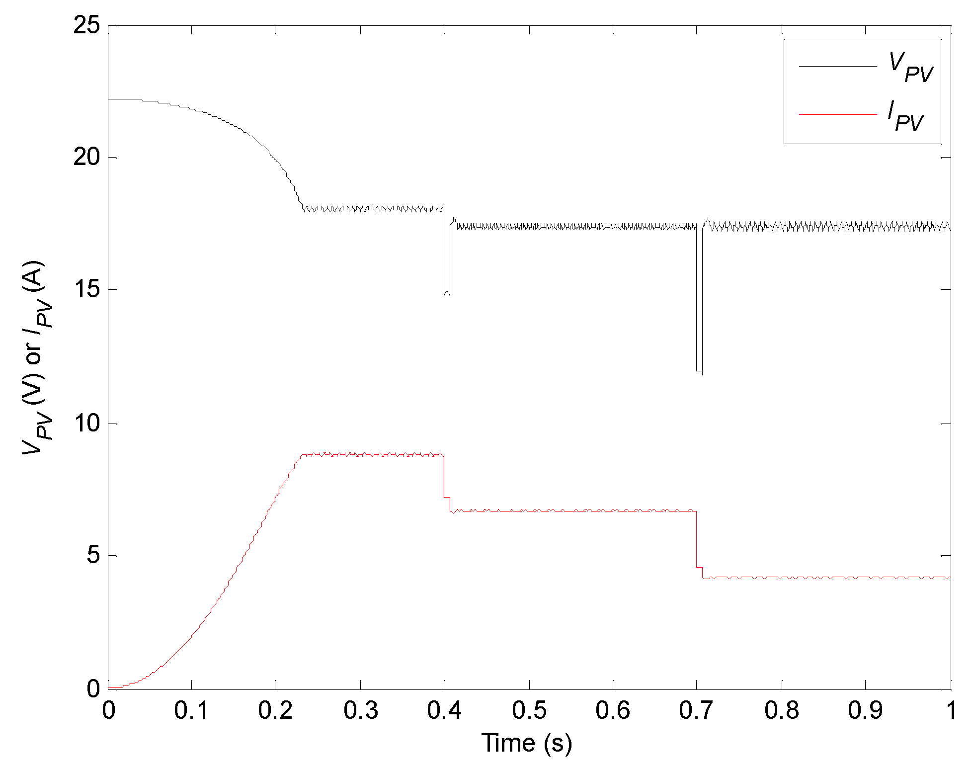
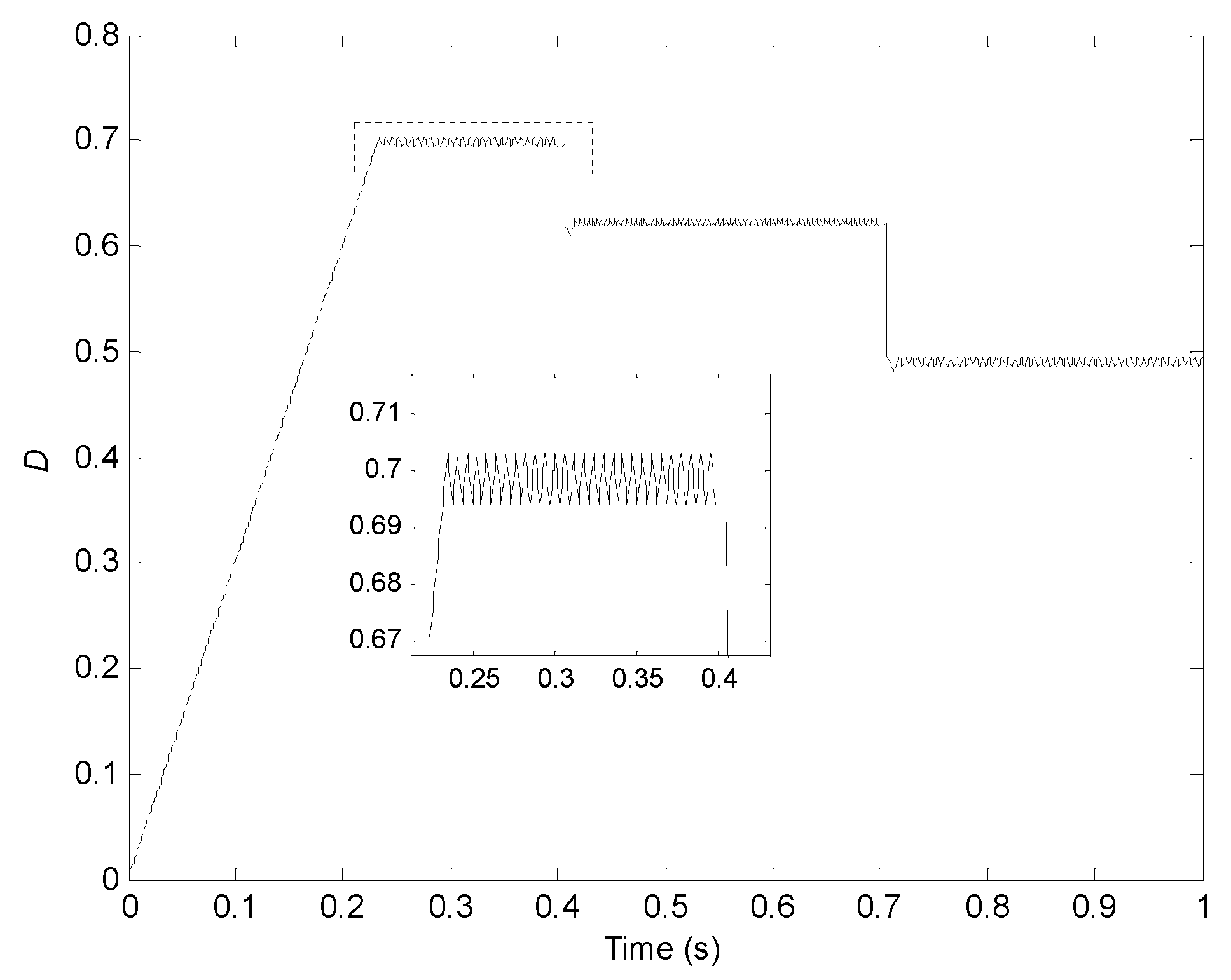
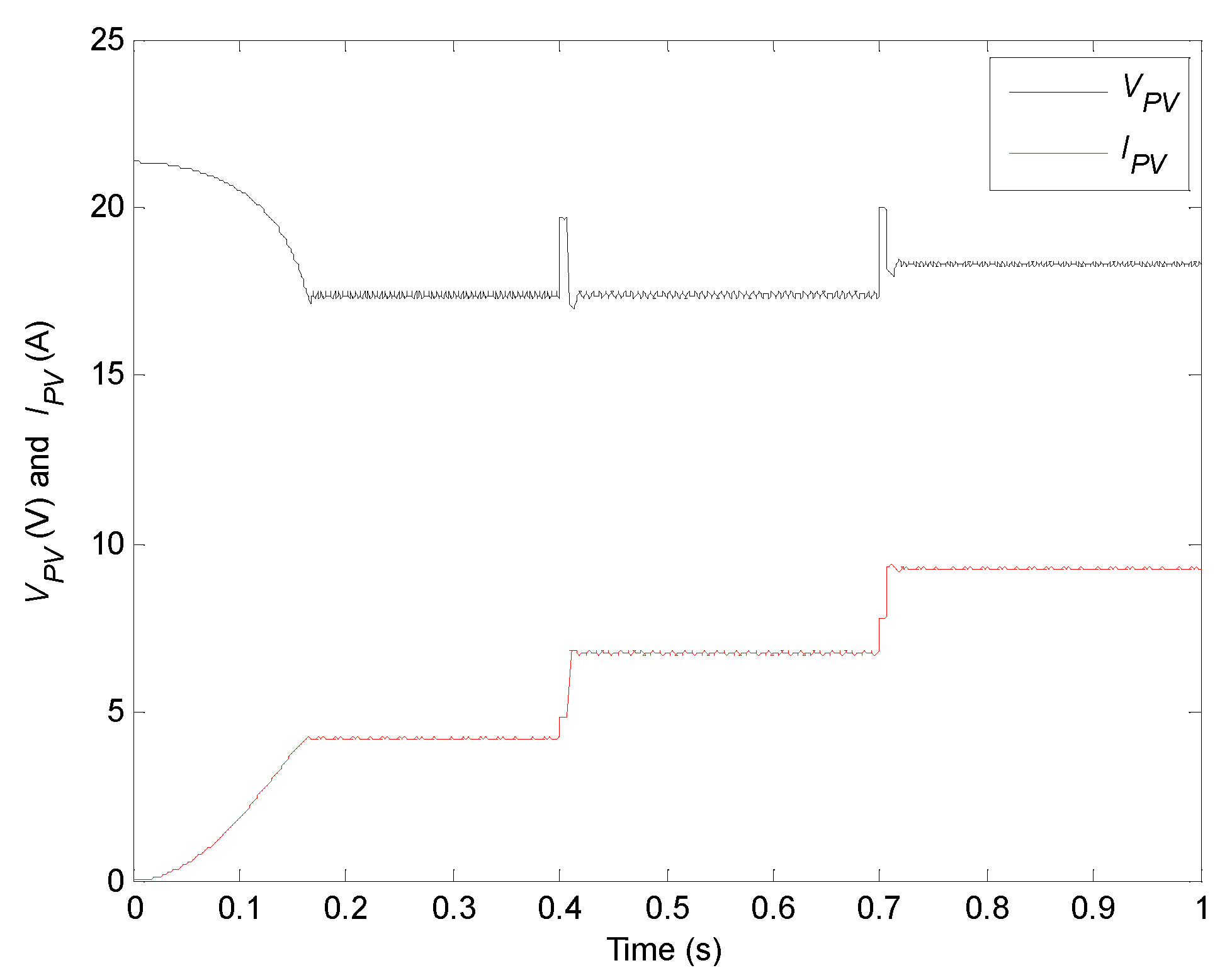
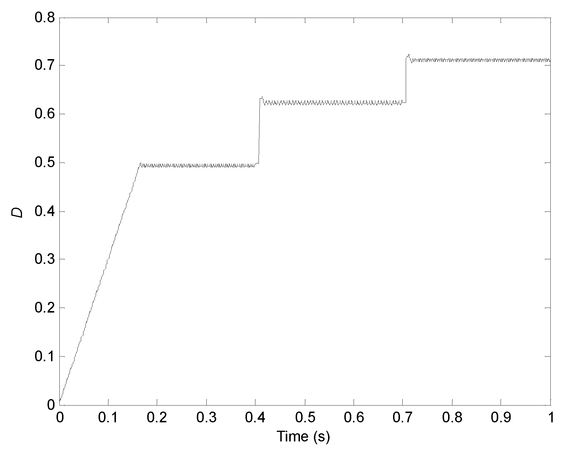
5. Simulation Experiments
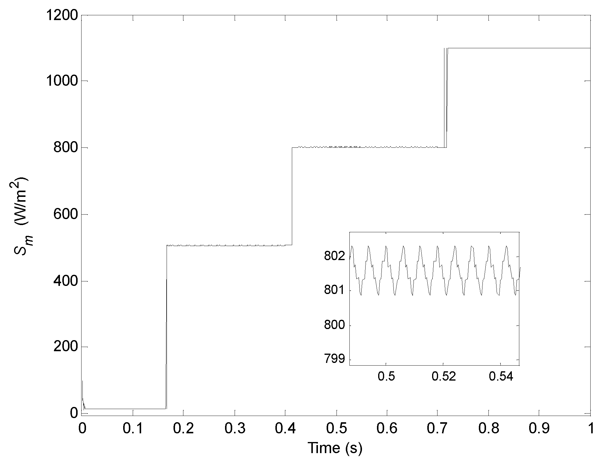
5.1. Estimation Method under Changeless Weather Conditions
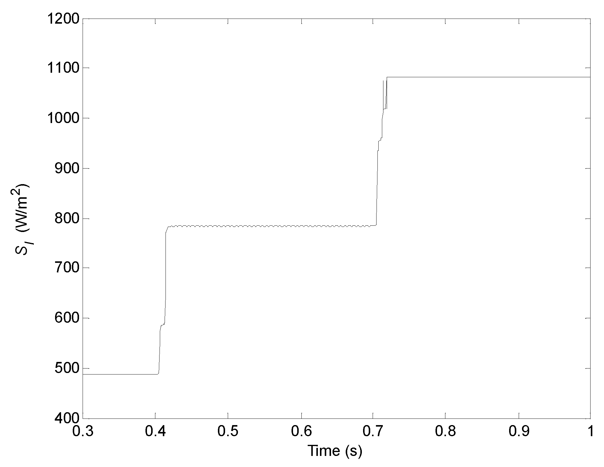
5.2. Estimation Method under Varying Weather Conditions
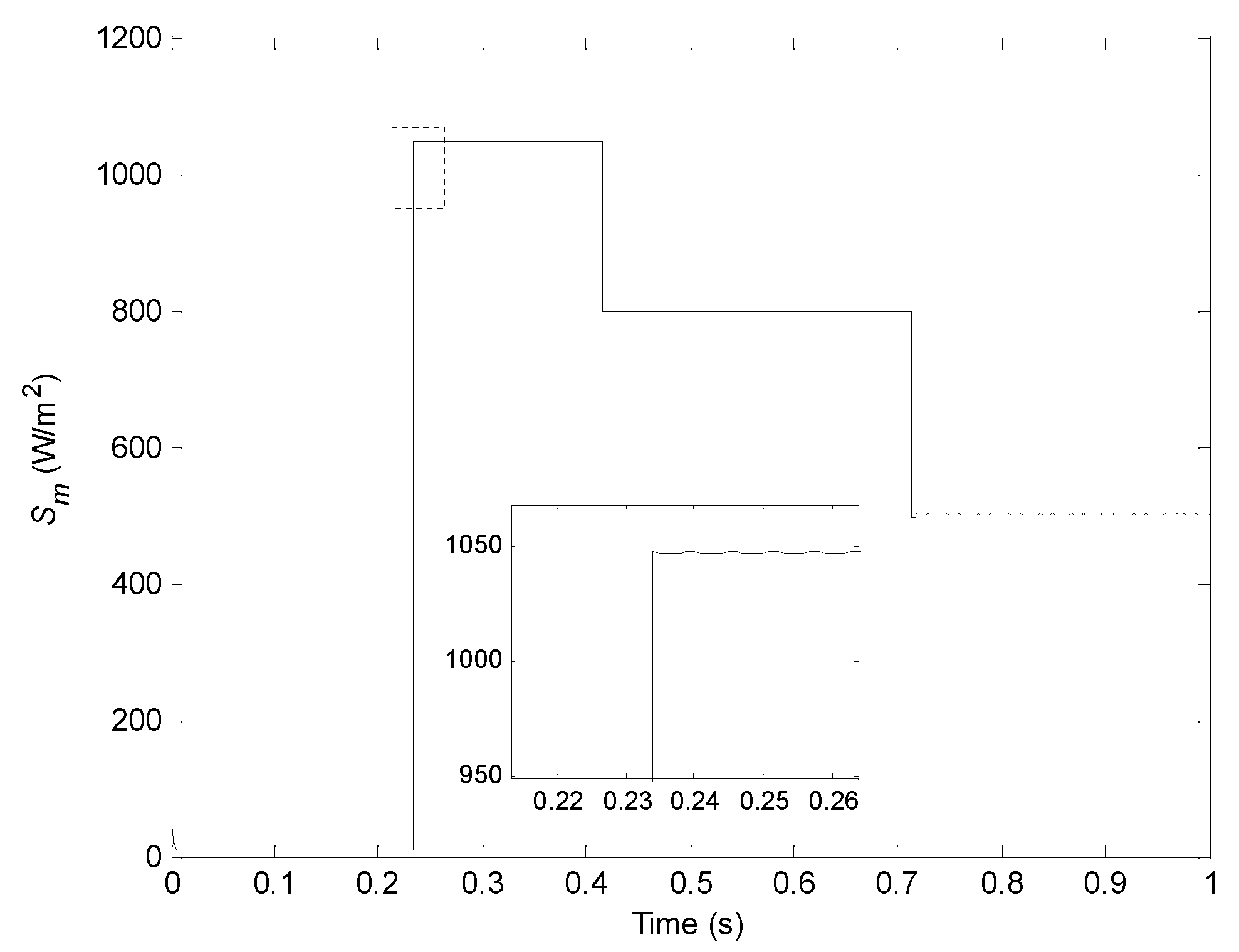
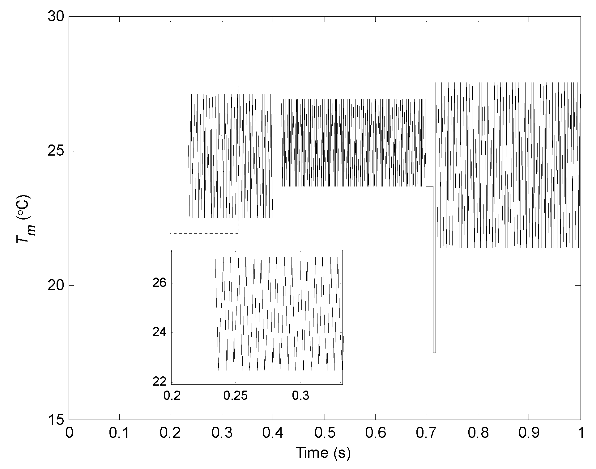
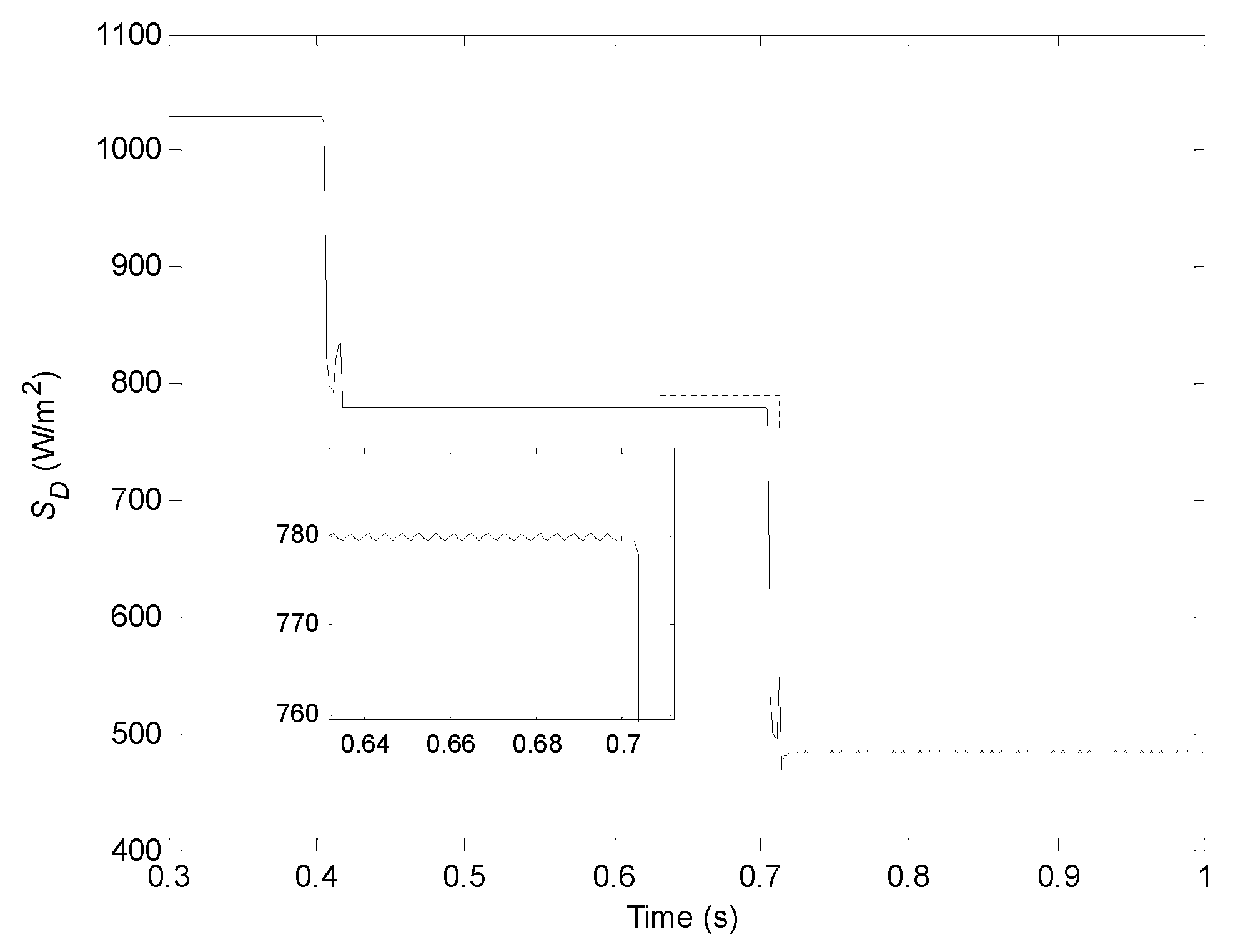
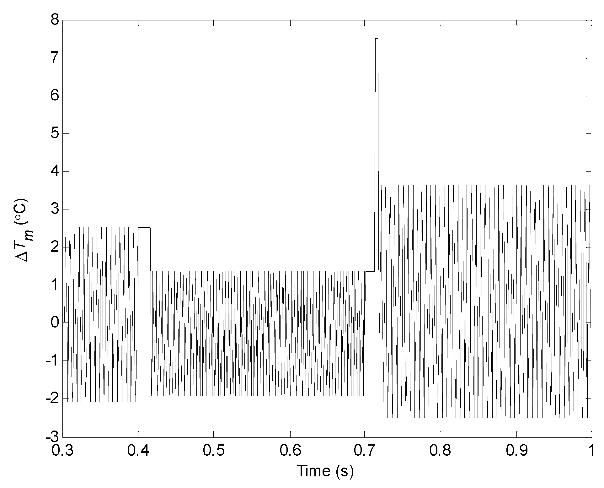
5.2.1. Simulation under Decreasing Irradiance Conditions
5.2.2. Simulation under Increasing Irradiance Conditions
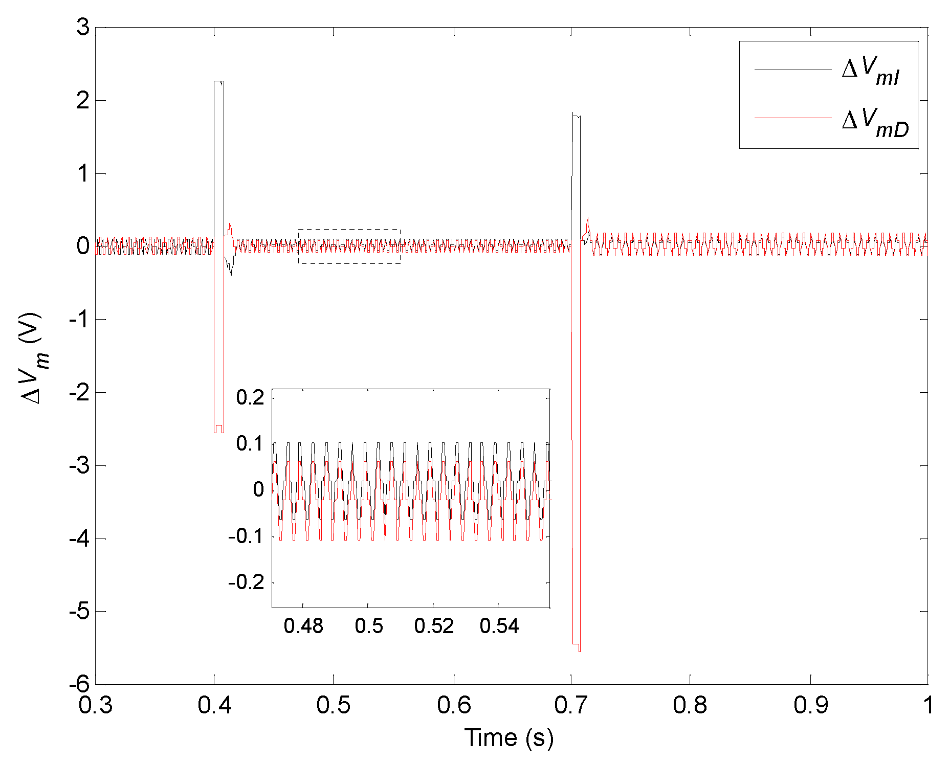
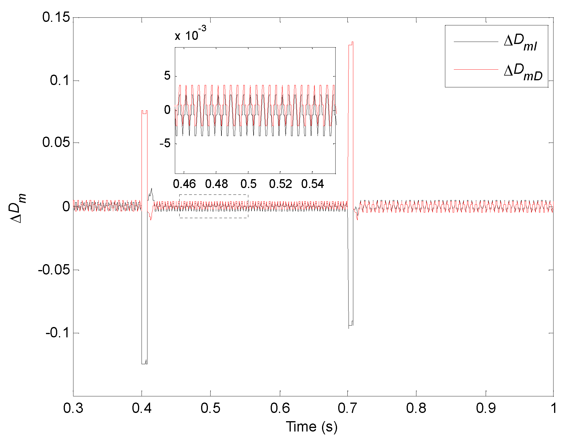
5.3. Feasibility, Availability, and Accuracy of the VWPOS
5.3.1. Accuracy of the Main Control Variables
5.3.2. Analysis of the Control Signal and Output Power
5.4. MPPT Optimization Effect of the VWPOS
5.4.1. Influence of the Different Tracking Step Sizes
5.4.2. Comparison with Other MPPT Methods
6. Discussions
7. Conclusions
Funding
Acknowledgments
Conflicts of Interest
Abbreviations
| MPPT | maximum power point tracking |
| VWP | variable-weather-parameter |
| MPP | maximum power point |
| PV | photovoltaic |
| PWM | pulse-width modulation |
| STC | standard test conditions |
| P&O | perturbation and observation |
| FLC | fuzzy logic control |
| PSO | particle swarm optimization |
| INC | incremental conduction |
| VWPOS | VWP optimization strategy |
| I&T | irradiance and temperature |
| Nomenclature | |
| Isc | short circuit current at STC (A) |
| Im | MPP current at STC (A) |
| Voc | open circuit voltage at STC (V) |
| Vm | MPP voltage at STC (V) |
| VPV | output voltage of PV cell (V) |
| IPV | output current of PV cell (A) |
| S | solar irradiance (W/m2) |
| T | cell temperature (°C) |
| RL | load resistance (Ω) |
| Po | output power of PV system (W) |
| D | duty cycle of the PWM signal of the DC/DC converter |
| C | VPV corresponding to the MPP of PV system (V) |
| Pomax | ideal or calculated value of the maximum output power (W) |
| PomaxP | maximum output power using the proposed strategy (W) |
| Pomax& | maximum output power using the P&O method with 0.003 step size (W) |
| PomaxP1 | PomaxP when the step size of the optimized P&O method is 0.003 (W) |
| PomaxP2 | PomaxP when the step size of the optimized P&O method is 0.002 (W) |
| PomaxV | maximum output power using the VWP method 1 in Ref. [5] (W) |
| Dmax | ideal or calculated value of the duty cycle at the MPP |
| DmaxP | duty cycle at the MPP using the proposed strategy |
| Dmax& | duty cycle at the MPP using the P&O method |
| DmaxP1 | DmaxP corresponding to PomaxP1 |
| DmaxP2 | DmaxP corresponding to PomaxP2 |
| DmaxV | duty cycle at the MPP using the VWP method 1 in Ref. [5] |
| settling time corresponding to PomaxP1 (ms) | |
| settling time corresponding to PomaxP2 (ms) | |
| settling time corresponding to Pomax& (ms) | |
| settling time corresponding to PomaxV (ms) | |
References
- Belkaid, A.; Colak, I.; Isik, O. Photovoltaic maximum power point tracking under fast varying of solar radiation. Appl. Energy 2016, 179, 523–530. [Google Scholar] [CrossRef]
- Danandeh, M.A.; Mousavi, G.S.M. Comparative and comprehensive review of maximum power point tracking methods for PV cells. Renew. Sustain. Energy Rev. 2018, 82, 2743–2767. [Google Scholar] [CrossRef]
- Li, X.; Wen, H.; Hu, Y.; Jiang, L. A novel beta parameter based fuzzy-logic controller for photovoltaic MPPT application. Renew. Energy 2019, 130, 416–427. [Google Scholar] [CrossRef]
- Hong, Y.-Y.; Beltran, A.A., Jr.; Paglinawan, A.C. A robust design of maximum power point tracking using Taguchi method for stand-alone PV system. Appl. Energy 2018, 211, 50–63. [Google Scholar] [CrossRef]
- Gao, X.; Li, S.; Gong, R. Maximum power point tracking control strategies with variable weather parameters for photovoltaic generation systems. Sol. Energy 2013, 93, 357–367. [Google Scholar] [CrossRef]
- Li, S. A maximum power point tracking method with variable weather parameters based on input resistance for photovoltaic system. Energy Convers. Manag. 2015, 106, 290–299. [Google Scholar] [CrossRef]
- Li, S. A variable-weather-parameter MPPT control strategy based on MPPT constraint conditions of PV system with inverter. Energy Convers. Manag. 2019, 197, 111873. [Google Scholar] [CrossRef]
- Sher, H.A.; Murtaza, A.F.; Noman, A.; Addoweesh, K.E.; Al-Haddad, K.; Chiaberge, M. A new sensorless hybrid MPPT algorithm based on fractional short-circuit current measurement and P&O MPPT. IEEE Trans. Sustain. Energy 2015, 6, 1426–1434. [Google Scholar]
- Li, S. A MPPT speed optimization strategy for photovoltaic system using VWP interval based on weather forecast. Optik 2019, 192, 162958. [Google Scholar] [CrossRef]
- Guo, S.; Abbassi, R.; Jerbi, H.; Rezvani, A.; Suzukie, K. Efficient maximum power point tracking for a photovoltaic using hybrid shufflfled frog-leaping and pattern search algorithm under changing environmental conditions. J. Clean. Prod. 2021, 297, 126573. [Google Scholar] [CrossRef]
- Yang, B.; Yu, T.; Shu, H.; Zhu, D.; An, N.; Sang, Y.; Jiang, L. Perturbation observer based fractional-order sliding-mode controller for MPPT of grid-connected PV inverters: Design and real-time implementation. Control Eng. Pract. 2018, 79, 105–125. [Google Scholar] [CrossRef]
- Veerapen, S.; Wen, H.; Li, X.; Du, Y.; Yang, Y.; Wang, Y.; Xiao, W. A novel global maximum power point tracking algorithm for photovoltaic system with variable perturbation frequency and zero oscillation. Sol. Energy 2019, 181, 345–356. [Google Scholar] [CrossRef]
- Bahrami, M.; Gavagsaz-Ghoachani, R.; Zandi, M.; Phattanasak, M.; Maranzanaa, G.; Nahid-Mobarakeh, B.; Pierfederici, S.; Meibody-Tabar, F. Hybrid maximum power point tracking algorithm with improved dynamic performance. Renew. Energy 2019, 130, 982–991. [Google Scholar] [CrossRef]
- Dehghani, M.; Taghipour, M.; Gharehpetian, G.B.; Abedi, M. Optimized fuzzy controller for MPPT of grid-connected PV systems in rapidly changing atmospheric conditions. J. Mod. Power Syst. Clean Energy 2021, 9, 376–383. [Google Scholar] [CrossRef]
- Zhang, X.; Gamage, D.; Wang, B.; Ukil, A. Hybrid maximum power point tracking method based on iterative learning control and perturb & observe method. IEEE Trans. Sustain. Energy 2021, 12, 659–670. [Google Scholar]
- Rezk, H.; AL-Oran, M.; Gomaa, M.R.; Tolba, M.A.; Fathy, A.; Ali Abdelkareem, M.; Olabi, A.G.; El-Sayed, A.H.M. A novel statistical performance evaluation of most modern optimization based global MPPT techniques for partially shaded PV system. Renew. Sustain. Energy Rev. 2019, 115, 109372. [Google Scholar] [CrossRef]
- Lasheen, M.; Abdel-Salam, M. Maximum power point tracking using hill climbing and ANFIS techniques for PV applications: A review and a novel hybrid approach. Energy Convers. Manag. 2018, 171, 1002–1019. [Google Scholar] [CrossRef]
- Cavalcanti, M.C.; Bradaschia, F.; do Nascimento, A.J., Jr.; Azevedo, G.M.S.; Barbosa, E.J. Hybrid maximum power point tracking technique for PV modules based on a double-diode model. IEEE Trans. Ind. Electron. 2021, 68, 8169–8181. [Google Scholar] [CrossRef]
- Killi, M.; Samanta, S. Modified perturb and observe MPPT algorithm for drift avoidance in photovoltaic systems. IEEE Trans. Ind. Electron. 2015, 62, 5549–5559. [Google Scholar] [CrossRef]
- Manoharan, P.; Subramaniam, U.; Babu, T.S.; Padmanaban, S.; Holm-Nielsen, J.B.; Mitolo, M.; Ravichandran, S. Improved perturb and observation maximum power point tracking technique for solar photovoltaic power generation systems. IEEE Syst. J. 2021, 15, 3024–3035. [Google Scholar] [CrossRef]
- Mutoh, N.; Ohno, M.; Inoue, T. A method for MPPT control while searching for parameters corresponding to weather conditions for PV generation systems. IEEE Trans. Ind. Electron. 2006, 53, 1055–1065. [Google Scholar] [CrossRef]
- Li, Q.; Zhao, S.; Wang, M.; Zou, Z.; Wang, B.; Chen, Q. An improved perturbation and observation maximum power point tracking algorithm based on a PV module four-parameter model for higher efficiency. Appl. Energy 2017, 195, 523–537. [Google Scholar] [CrossRef]
- Gopi, R.; Sreejith, S. Converter topologies in photovoltaic applications—A review. Renew. Sustain. Energy Rev. 2018, 94, 1–14. [Google Scholar] [CrossRef]


| S (W/m2) | 200 | 300 | 400 | 500 | 600 | 700 | 800 | 900 | 1000 | 1100 | 1200 |
|---|---|---|---|---|---|---|---|---|---|---|---|
| Pomax (W) | 30.65 | 44.90 | 59.04 | 73.15 | 87.33 | 102.02 | 117.27 | 133.47 | 150.83 | 169.45 | 189.48 |
| Dmax | 0.3001 | 0.3705 | 0.4314 | 0.4852 | 0.5327 | 0.5754 | 0.6131 | 0.6466 | 0.6761 | 0.7018 | 0.7239 |
| T (°C) | 0 | 5 | 10 | 15 | 20 | 25 | 30 | 35 | 40 | 45 | 50 |
|---|---|---|---|---|---|---|---|---|---|---|---|
| Pomax (W) | 117.74 | 117.54 | 117.62 | 117.47 | 117.27 | 117.16 | 116.73 | 116.63 | 116.21 | 115.91 | 115.48 |
| Dmax | 0.5813 | 0.5887 | 0.5971 | 0.6050 | 0.6131 | 0.6216 | 0.6295 | 0.6386 | 0.6470 | 0.6561 | 0.6650 |
| RL (Ω) | 0.4 | 0.6 | 0.8 | 1.0 | 1.2 | 1.4 | 1.6 | 1.8 | 2.0 |
|---|---|---|---|---|---|---|---|---|---|
| Pomax (W) | 117.06 | 117.28 | 117.18 | 117.27 | 117.25 | 117.32 | 117.34 | 117.35 | 117.31 |
| Dmax | 0.3874 | 0.4749 | 0.5481 | 0.6131 | 0.6716 | 0.7256 | 0.7757 | 0.8228 | 0.8672 |
| SI (W/m2) | 400 | 500 | 600 | 700 | 800 | 900 | 1000 | 1100 | 1200 | |
|---|---|---|---|---|---|---|---|---|---|---|
| Sm = 300 (W/m2) | Po (W) | 52.96 | 55.60 | 57.02 | 58.31 | 59.85 | 61.83 | 64.34 | 67.44 | 71.15 |
| Sm = 400 (W/m2) | Po (W) | / | 68.22 | 72.45 | 75.34 | 78.08 | 81.16 | 84.81 | 89.16 | 94.28 |
| Sm = 500 (W/m2) | Po (W) | / | / | 83.40 | 89.38 | 94.08 | 98.69 | 103.74 | 109.50 | 116.11 |
| Sm = 600 (W/m2) | Po (W) | / | / | / | 98.74 | 106.60 | 113.38 | 120.19 | 127.56 | 135.78 |
| Sm = 700 (W/m2) | Po (W) | / | / | / | / | 114.67 | 124.57 | 133.68 | 142.97 | 152.96 |
| Sm = 800 (W/m2) | Po (W) | / | / | / | / | / | 131.36 | 143.39 | 154.96 | 166.92 |
| Sm = 900 (W/m2) | Po (W) | / | / | / | / | / | / | 149.09 | 163.34 | 177.49 |
| Sm = 1000 (W/m2) | Po (W) | / | / | / | / | / | / | / | 168.06 | 184.59 |
| SD (W/m2) | 900 | 800 | 700 | 600 | 500 | 400 | 300 | |
|---|---|---|---|---|---|---|---|---|
| Sm = 1000 (W/m2) | Po (W) | 131.81 | 110.09 | 86.81 | 64.52 | 44.97 | 28.81 | 16.21 |
| Sm = 900 (W/m2) | Po (W) | / | 115.17 | 93.28 | 70.20 | 49.12 | 31.50 | 17.73 |
| Sm = 800 (W/m2) | Po (W) | / | / | 99.325 | 77.05 | 54.47 | 35.01 | 19.71 |
| Sm = 700 (W/m2) | Po (W) | / | / | / | 84.01 | 61.30 | 39.70 | 22.38 |
| Sm = 600 (W/m2) | Po (W) | / | / | / | / | 69.05 | 46.08 | 26.09 |
| Sm = 500 (W/m2) | Po (W) | / | / | / | / | / | 54.09 | 31.38 |
| Operating Conditions | (1) | (2) | (3) | (4) | (5) | (6) | (7) | (8) |
|---|---|---|---|---|---|---|---|---|
| S (W/m2) | constant | varying | constant | constant | varying | constant | varying | varying |
| T (°C) | constant | constant | varying | constant | varying | varying | constant | varying |
| RL (Ω) | constant | constant | constant | varying | constant | varying | varying | varying |
| Weather Conditions (W/m2, °C) | (V) | (A) | Sm (W/m2) | Tm (°C) | ΔSm (W/m2) | ΔTm (°C) | |
| (300,10) | 0.442 | 8.231 | 5.487 | 299.358 | 9.415 | 0.642 | 0.585 |
| (300,20) | 0.454 | 8.221 | 5.481 | 301.759 | 19.221 | −1.759 | 0.779 |
| (450,10) | 0.547 | 9.974 | 6.649 | 450.821 | 9.679 | −0.821 | 0.321 |
| (450,20) | 0.562 | 9.963 | 6.642 | 452.867 | 19.524 | −2.867 | 0.476 |
| (550,15) | 0.616 | 10.981 | 7.320 | 551.548 | 15.233 | −1.548 | −0.233 |
| (550,22) | 0.628 | 10.970 | 7.313 | 552.600 | 22.156 | −2.600 | −0.156 |
| (650,20) | 0.679 | 11.916 | 7.944 | 651.019 | 19.855 | −1.019 | 0.145 |
| (650,28) | 0.694 | 11.899 | 7.933 | 651.556 | 27.753 | −1.556 | 0.247 |
| (800,25) | 0.761 | 13.256 | 8.838 | 799.550 | 24.899 | 0.450 | 0.101 |
| (800,30) | 0.772 | 13.243 | 8.829 | 799.466 | 29.906 | 0.534 | 0.094 |
| (800,35) | 0.783 | 13.226 | 8.817 | 799.018 | 34.785 | 0.982 | 0.215 |
| (950,25) | 0.822 | 14.585 | 9.723 | 948.904 | 24.719 | 1.096 | 0.281 |
| (950,35) | 0.844 | 14.552 | 9.701 | 947.757 | 34.455 | 2.243 | 0.545 |
| (1050,30) | 0.868 | 15.462 | 10.308 | 1048.866 | 29.899 | 1.134 | 0.101 |
| (1050,40) | 0.892 | 15.421 | 10.281 | 1046.768 | 39.917 | 3.232 | 0.083 |
| (1180,35) | 0.917 | 16.623 | 11.082 | 1178.958 | 35.051 | 1.042 | −0.051 |
| (1180,40) | 0.931 | 16.600 | 11.066 | 1177.646 | 40.567 | 2.354 | −0.567 |
| Initial Values (W/m2) | Final Values (W/m2) | Dmax | DmaxP | Dmax& | Pomax (W) | PomaxP (W) | Pomax& (W) |
|---|---|---|---|---|---|---|---|
| 300 | 500 | 0.4919 | 0.4920 | 0.4915 | 73.083 | 70.767 | 70.755 |
| 300 | 1100 | 0.7113 | 0.7121 | 0.7120 | 169.171 | 165.638 | 165.647 |
| 500 | 800 | 0.6216 | 0.6209 | 0.6220 | 117.163 | 114.228 | 114.233 |
| 500 | 1100 | 0.7113 | 0.7104 | 0.7120 | 169.171 | 165.650 | 165.648 |
| 700 | 400 | 0.4377 | 0.4375 | 0.4376 | 59.069 | 56.985 | 56.977 |
| 700 | 900 | 0.6556 | 0.6555 | 0.6550 | 133.332 | 130.205 | 130.204 |
| 700 | 1100 | 0.7113 | 0.7118 | 0.7120 | 169.171 | 165.649 | 165.647 |
| 900 | 500 | 0.4919 | 0.4913 | 0.4915 | 73.083 | 70.764 | 70.755 |
| 900 | 600 | 0.5402 | 0.5423 | 0.5410 | 87.273 | 84.742 | 84.739 |
| 900 | 1100 | 0.7113 | 0.7108 | 0.7120 | 169.171 | 165.639 | 165.646 |
| 1000 | 800 | 0.6216 | 0.6210 | 0.6220 | 117.163 | 114.222 | 114.230 |
| 1000 | 600 | 0.5402 | 0.5400 | 0.5410 | 87.273 | 84.732 | 84.740 |
| 1000 | 500 | 0.4919 | 0.4918 | 0.4915 | 73.083 | 70.765 | 70.755 |
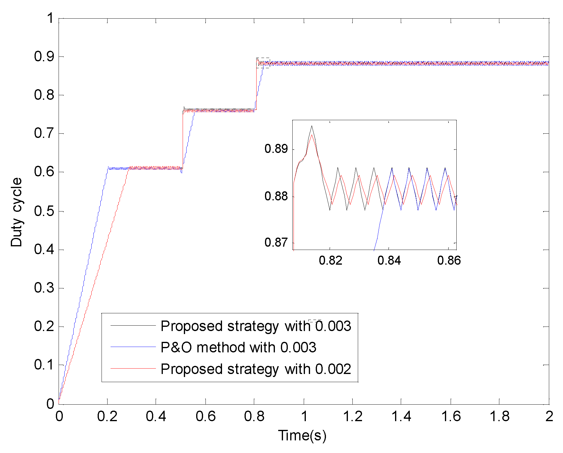
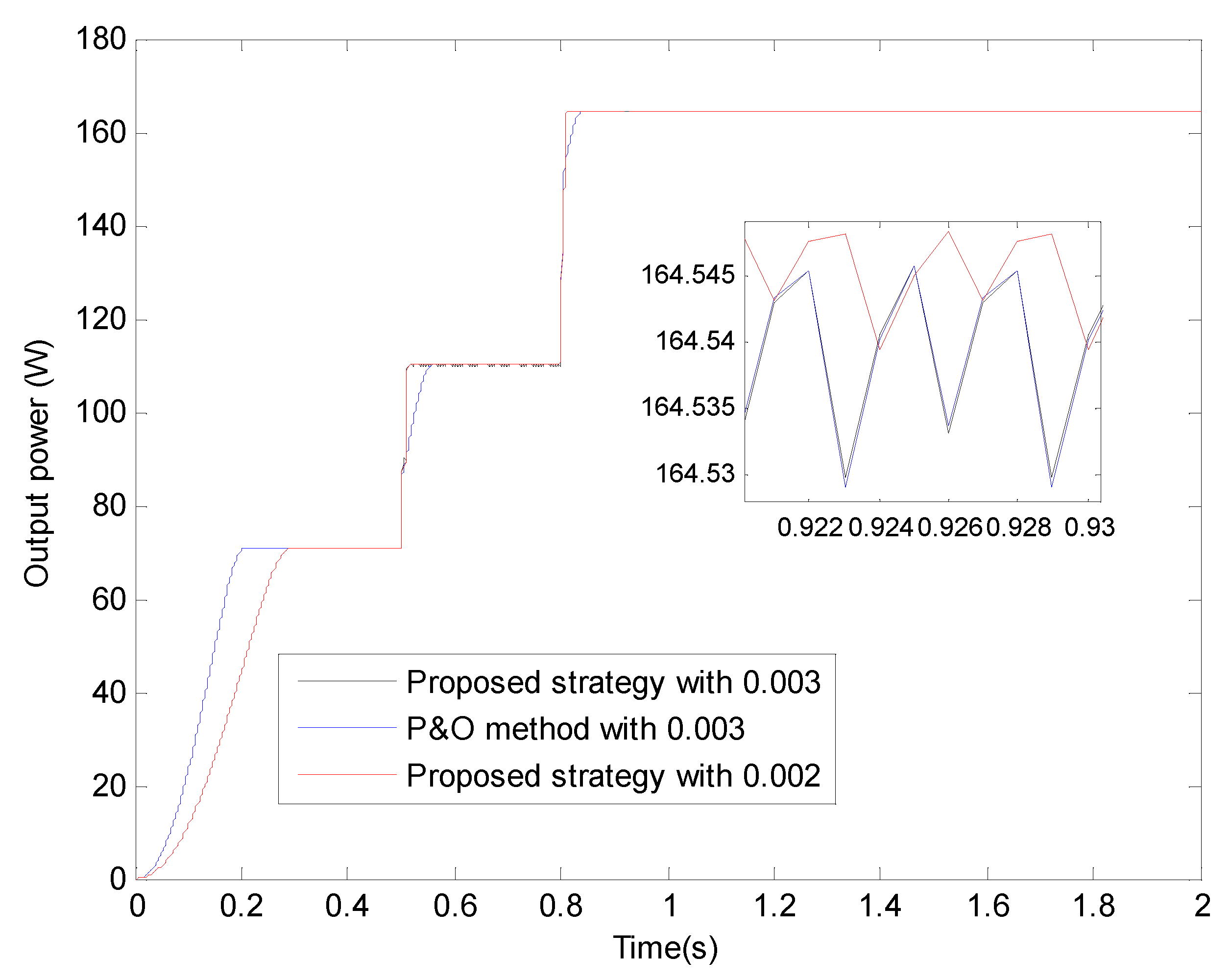
| Range of Time (s) | S (W/m2) | Dmax | Pomax (W) | DmaxP1 | DmaxP2 | Dmax& | Pomax1 (W) | Pomax2 (W) | Pomax& (W) | (ms) | (ms) | (ms) |
| [0, 0.5] | 500 | 0.6106 | 72.931 | 0.609 | 0.611 | 0.609 | 70.619 | 70.621 | 70.619 | / | / | 204 |
| [0.5, 0.8] | 774 | 0.7598 | 112.878 | 0.760 | 0.760 | 0.760 | 110.004 | 110.005 | 110.004 | 14 | 14 | 56 |
| [0.8, 2] | 1096 | 0.8818 | 168.051 | 0.882 | 0.882 | 0.882 | 164.539 | 164.545 | 164.539 | 13 | 13 | 40 |
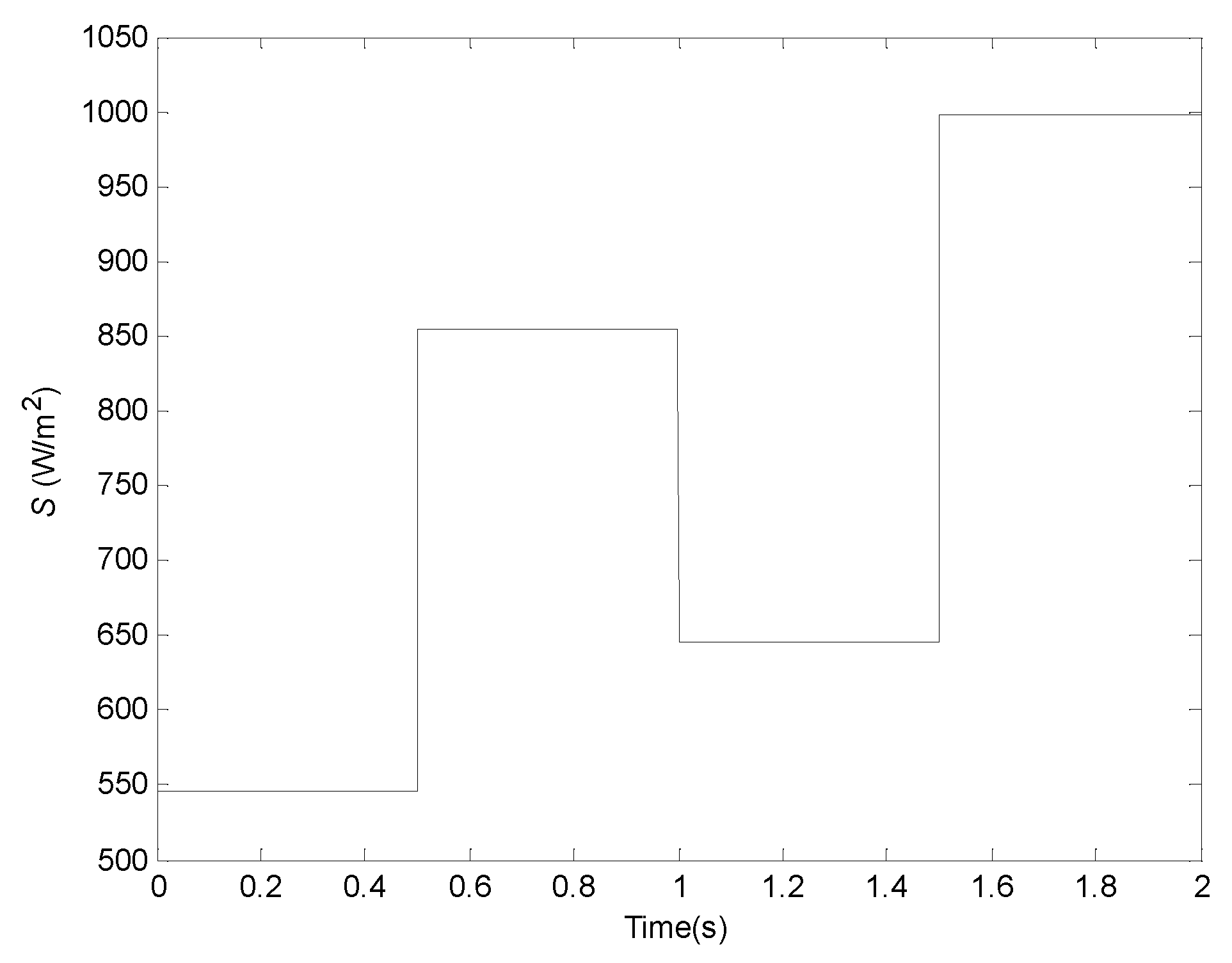
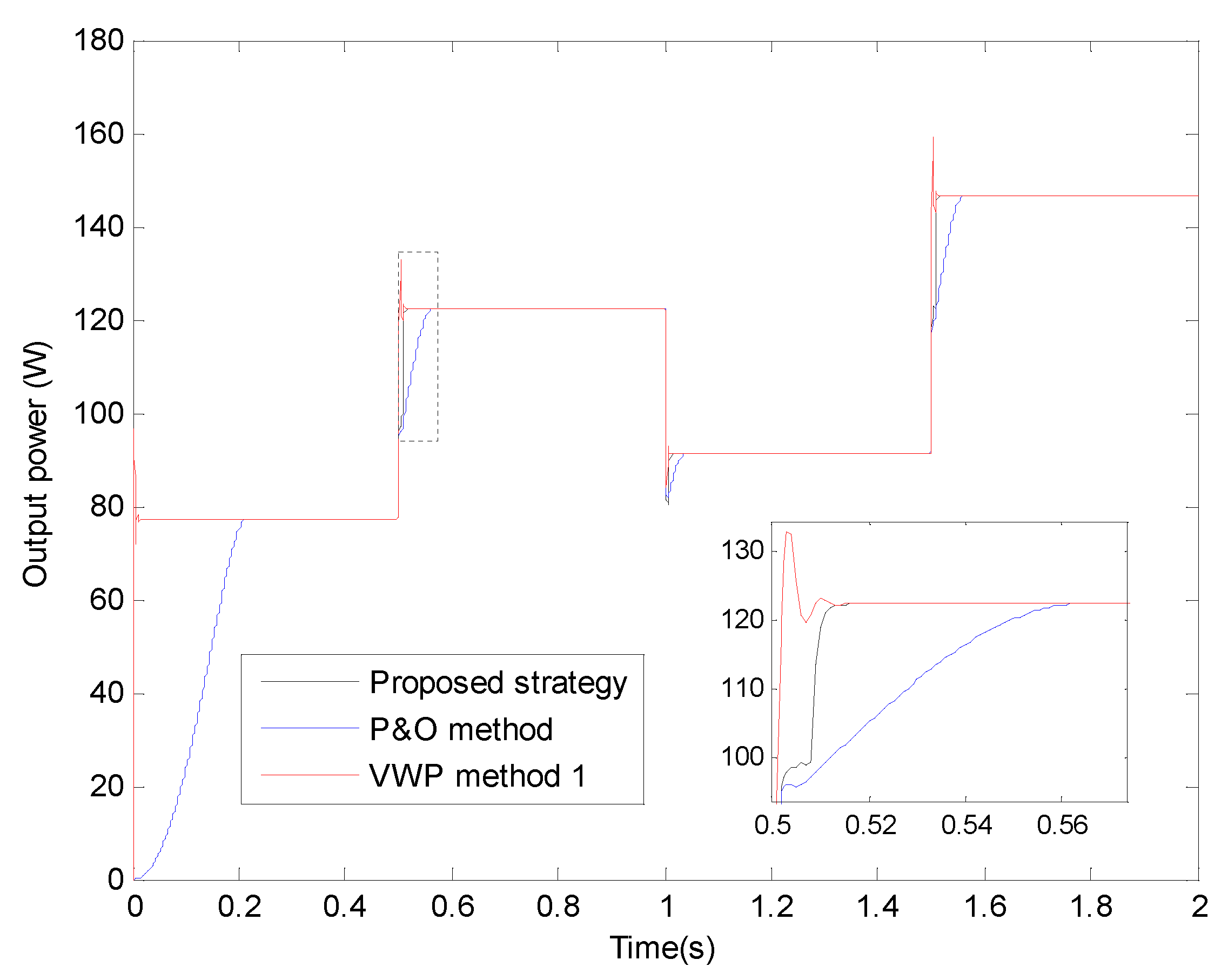
| Range of Time (s) | S (W/m2) | Dmax | Pomax (W) | DmaxP1 | Dmax& | DmaxV | PomaxP1 (W) | Pomax& (W) | PomaxV (W) | (ms) | (ms) | (ms) |
| [0.3, 0.5] | 546 | 0.6391 | 79.408 | 0.6380 | 0.6380 | 0.6375 | 76.991 | 76.991 | 76.999 | / | 214 | 18 |
| [0.5, 1] | 854 | 0.7951 | 125.508 | 0.7940 | 0.7940 | 0.7962 | 122.477 | 122.474 | 122.481 | 16.5 | 64 | 14 |
| [1, 1.5] | 646 | 0.6959 | 93.732 | 0.6950 | 0.6950 | 0.6953 | 91.108 | 91.105 | 91.118 | 12 | 37 | 17 |
| [1.5, 2] | 998 | 0.8501 | 149.935 | 0.8502 | 0.8502 | 0.8514 | 146.622 | 146.623 | 146.627 | 14 | 62 | 16 |
| MPPT Methods or Strategies | Main Advantages | Main Disadvantages |
| VWPOS |
|
|
| P&O method |
|
|
| FLC method |
|
|
| VWP method 1 |
|
|
Publisher’s Note: MDPI stays neutral with regard to jurisdictional claims in published maps and institutional affiliations. |
© 2022 by the author. Licensee MDPI, Basel, Switzerland. This article is an open access article distributed under the terms and conditions of the Creative Commons Attribution (CC BY) license (https://creativecommons.org/licenses/by/4.0/).
Share and Cite
Li, S. A Variable-Weather-Parameter Optimization Strategy Based on an Irradiance and Temperature Estimation Method for PV System. Electronics 2022, 11, 1439. https://doi.org/10.3390/electronics11091439
Li S. A Variable-Weather-Parameter Optimization Strategy Based on an Irradiance and Temperature Estimation Method for PV System. Electronics. 2022; 11(9):1439. https://doi.org/10.3390/electronics11091439
Chicago/Turabian StyleLi, Shaowu. 2022. "A Variable-Weather-Parameter Optimization Strategy Based on an Irradiance and Temperature Estimation Method for PV System" Electronics 11, no. 9: 1439. https://doi.org/10.3390/electronics11091439
APA StyleLi, S. (2022). A Variable-Weather-Parameter Optimization Strategy Based on an Irradiance and Temperature Estimation Method for PV System. Electronics, 11(9), 1439. https://doi.org/10.3390/electronics11091439