Abstract
An increasing number of battery-powered devices that are used outdoors or in mobile systems put emphasis on the power and energy efficiency as a form of trade-off between application performance and system power consumption. However, lack of objective metrics for the evaluation of application performance degradation poses difficulties for managing such trade-offs in real-time applications. The proposed methodology introduces metrics for modeling of application performance and the technique for its control, enabling more efficient power–performance trade-off management. The methodology allows for selective system performance degradation and fine-grained control of system behavior in the power–performance domain by extending the set of operating point parameters controllable through real-time application. The utilization and the effectiveness of the proposed methodology is evaluated in a simulated environment for different scenarios of the application execution, including system operation above the utilization bounds.
1. Introduction
In recent years, the Internet of Things (IoT) has gained popularity as an increasing number of embedded devices are being integrated in the global network [1]. It is expected that by the year 2025, the number of connected devices will reach 75 billion, with the expected growth rate near 10% per year [2]. As there is an emphasis on energy efficiency in today’s world, reducing energy consumption is found as a common goal in designing such devices, as well as any electronic systems. As most devices are offering the services that rely on battery powered mobile, handheld, portable, and wearable platforms, the requirements for prolonged battery life further elevate the importance of efficient energy usage [3,4,5]. Furthermore, the requirement of portability itself poses restrictions on the size and weight of such devices and consequently limits the availability of energy resources on such devices. Additionally, many of these devices are placed outdoors in harsh or inaccessible environments, which often makes battery replacement or charging unrealistic or impractical. Therefore, optimizing battery lifetime has become one of the key challenges in designing battery-powered embedded devices. Other non-portable embedded systems, either grid connected or consuming generator power, are also expected to optimize total energy and power usage and avoid excess heat generation. Nevertheless, motives for low power design and more efficient utilization of energy resources can be found for various pragmatic, economic, technical, and environmental reasons [4,6,7].
From the context of optimizing embedded system operation, efficiency can be seen as a form of trade-off between the system performance and the utilization of system resources. A common goal in designing such a system is to minimize power needs delivering the required set of functionalities or to utilize a reduced amount of energy to perform the same assignments. From a similar viewpoint, low power design can be noted as a pragmatic approach for optimizing power and energy consumption. Therefore, many power management techniques are proposed to keep up with the low power system design targeting management of a system’s power or energy resources [8,9].
Modern embedded controllers and other IC components allow designers to control power consumption through different power management strategies using available power-saving features and low-power operation modes. Universally, low power design intends to reduce the overall dynamic and static power consumption using a collection of techniques and methodologies [4]. Although the traditional approaches for designing low-power embedded systems vary, from simply relying on semiconductor manufacturers offering low power products, to more complex workload scheduling, there is no single universally accepted methodology applicable in all use cases. Ordinarily, it is a combination of component, circuit, system, application design, and associated trade-offs [8,10,11,12,13,14]. In general, extensive optimization of embedded systems for low power consumption requires balancing between the application performance and system power usage. It should be kept in mind that using the techniques for reducing power consumption may affect application performance in a way that compromises reliability and overall system capabilities.
Microprocessor and microcontroller manufacturers are offering different options for balancing the processing workload against consumed power. A common solution to bridge the gap between high performance and low power is to allow processors to run at different performance levels depending on the current workload [13,15,16]. In addition, standard operating systems (OSs) are offering services, dedicated for general purpose applications, to coordinate power management activities based on power policy settings.
The comprehensive survey given in [8] shows how the proposed power management solutions mature to address the evolution of the platform’s features and application needs. In addition to giving the properties and discussing the effectiveness of different power management techniques, it also presents a taxonomy to classify the existing approaches for uniprocessor systems, distinguishing them according to the underlying technology exploited for reducing energy consumption. However, the proposed solutions usually do not fit into safety-critical and real-time systems based on deeply embedded platforms with constrained processing and memory resources. Additionally, approaches that suggest the change of scheduling strategy or adopting OS to support power management are rather complex and power demanding because they involve additional processing. This forms the disparity in the wide applicability of the solution on the existing embedded platforms managed by real-time OS (RTOS) [17]. Evidencing further the research gap, we found that the lack of quantifiable performance metrics poses difficulties for the practical application of arbitrary trade-off management technique because there is no direct link between the power and performance domains. Unlike power savings, which can be easily measured and quantified, there is no objective measure of application performance, which has mostly been done through subjective evaluation [18,19,20]. Furthermore, standard power management techniques, regardless of the scope of the system parameters that they affect, like in voltage and frequency scaling [3,19,20,21,22,23,24,25], or approach in the domain of task scheduling that is employed [5,8,16,26,27,28,29,30,31,32], adopt inflexible criterion for application execution without deadline misses of individual tasks. The adopted criteria are inflexible as they are evaluated from the worst-case execution scenario, although actual system performances significantly vary depending on the appearance of external events. The aperiodic or sporadic nature of external events poses additional challenges in estimating actual application performance, as well as sustaining the deterministic system behavior during potential transient overloads [31].
The background for the proposed performance estimation methodology is found in the theory of real-time systems, where several types of tasks are identified according to their deadline strictness, i.e., the soft, firm, and hard real-time tasks. Following the definition of soft and firm real-time tasks, where failures to meet few deadlines of these tasks will not lead to total system failure, but degrades the system performance, opens the prospects for monitored performance degradation. This ability of maintaining the required level of functionality and to continue system operation, possibly at the reduced level, rather than deteriorating completely, is referred to as the graceful degradation concept [11,12,14,15,16]. Investigating the domain of fault-tolerant systems, several application classes are identified [5,15,16,24,33,34,35,36] where performance degradation is tolerated.
In approximate computing [33], some task instances can be omitted without compromising system operation. Imprecise computation [34,35] splits tasks into mandatory and best-effort parts. Mandatory parts must execute every time, but best-effort parts can be skipped. In multimedia applications [36], some frames can be skipped without affecting overall quality. Adopted from mixed-criticality systems, there are several research studies and solutions targeting real-time scheduling by introducing mixed-criticality task models, analyzing different issues in safety-critical applications, performing multi-criticality analysis [11,12], etc. However, all these attempts lack systematic and objective metrics for quantifying performance degradation and ability for fine-grained selective power–performance trade-off applicable on standard RTOS platforms.
This paper introduces the methodology for managing the real-time embedded system operation in the power–performance domain. The presented approach facilitates overcoming the limitations in the applicability of available approaches and their effectiveness in optimizing energy efficiency of an arbitrary RTOS-based application. The methodology introduces objective task-level performance metrics for the application-level performance assessment and the utilization control technique (UCT) for fine-grade management of power–performance trade-offs.
The immediate benefits and contributions of the proposed methodology are:
- Proposed task performance model for the quantification of task-level performance enables objective assessments of real-time application performance degradation and the detection of execution failures.
- The extension of system-level operating point parameters established the bound between power management and performance domains as a background for power-performance trade-offs. Tuning of operating point parameters can be carried out as a universal software solution in line with the adopted optimization criterion.
- Introduction of the utilization control technique enables fine-grained management of power–performance trade-off. At the same time, functional efficiency of system execution is retained because the application of UCT is not affecting the execution of safety critical tasks.
- Tuning of operating point parameters, through the combined UCT and DVFS approaches, enables more efficient operation of an embedded system in the power–performance domain, compared to system operation under the traditional DVFS power management.
- Implementation of UCT can be handled as a simple upgrade of the traditional RTOS with static priority-based scheduling. As an extension of the static scheduling approach, introduction of UCT preserves deterministic system behavior under transient overloads.
This paper is outlined as follows. In Section 2, a review of the most recent research efforts and available scientific studies addressing the low-power design, power management techniques, and approaches for more efficient energy utilization found in embedded computing applications and products is presented. Evaluation of found methodologies for performance analysis and the discussions of mixed-criticality and multi-criticality systems are also given. Details of the proposed approach for task-level performance estimation and modeling, application-level performance estimation, and the power management technique based on task-level utilization control, all as parts of the presented methodology for power–performance trade-off management, are given in Section 3. The results of the analysis of simulated system operation for different use case scenarios that validate and quantify contributions and benefits of the proposed UCT and combined UCT and DVFS approaches are given in Section 4. Concluding remarks and the directions for future work are given in Section 5.
2. Related Work
Power management and energy efficiency are key parameters in any system design and integration, especially valuable for mobile or size-constrained devices. Many research studies and scientific papers are addressing improved usage of energy and power resources on embedded platforms, introducing a variety of power management and low power design approaches, as well as guidelines for their implementation [4,6,37]. The common goal of the reviewed methodologies is to optimize the power budget providing the same level of services, and/or at the same time minimizing energy and power usage. Therefore, power management can be considered as a practical approach to improve energy and power efficiency of the system.
The rest of the section gives insight into the actual research efforts and the studies addressing different power management techniques to control power and energy usage, as well as challenges and limitations of their applicability.
Underlying methodologies for power management are applied at different design abstraction levels, from circuit to architectural and system level, optimizing hardware or/and software of an embedded system [4]. Static power management (SPM) techniques, such as synthesis and compilation for low power, are applied at design time, targeting both hardware and software. In contrast, dynamic power management (DPM) techniques optimize system runtime behavior to reduce power when systems are in idle or serving non-critical workloads. As the emphasis of our work is on dynamic approach, the rest of the section is focused on the available dynamic power management techniques and associated trade-offs.
Dynamic voltage and frequency scaling (DVFS) is a dominantly employed technique for reducing CPU power consumption [3,19,20,21,22,23,24,25]. Selection of the appropriate DVFS technique varies on the type of computing component, the timing and resources constraints, the application requirements, and the expected performance level. From the viewpoint of large-scale parallel application, the study given in [3] presents a model that gives an upper bound on performance loss due to frequency scaling impact on message passing interface (MPI) application performance. It analyzes how application sensitivity to frequency scaling evolved over the last decade for different cluster generations, at the same time targeting the energy effectiveness of the applied DVFS. Possible trade-offs between computing performance and energy efficiency, using DVFS on the latest many-core architecture processor suitable for high-performance computing (HPC) applications, is analyzed in [20]. The analyses include dependence of energy consumption for different data-layouts, memory configurations, and core settings.
From the viewpoint of a typical embedded application running on the microcontroller platform, the investigation presented in [25] proved that the impact of DVFS on the performance and power consumption may lead to the increase of up to 57% of the normalized power because of, e.g., inappropriate high voltage and frequency settings. As the efficiency depends on two factors, including power or energy consumption and runtime performance, many approaches combine the DVFS power optimization technique with scheduling approaches [8,21,22,23,25,26,27,28,29]. As given in the survey [8], targeting uniprocessor platforms, depending on the granularity of time instances when scaling is performed, DVFS can be characterized as intra-task or inter-task. In intra-task DVFS [21], scaling is done relative to the duration of execution of the task instances. In such scenarios, task instances start execution with lower frequency settings, and frequency is increased as a deadline approaches. In inter-task DVFS, if required, scaling is performed prior to the execution of the task instance [21,22,23].
The study presented in [21] investigates both intra-task and inter-task, as well as hybrid strategies for dynamic voltage scaling based on ideal and realistic system models with discrete settings of system parameters and included reconfiguration overheads. The results confirmed that the goal of minimizing the expected energy consumption in the system is achievable if the variability of the computational requirements of the workload can be captured by the for each task in the system. An algorithm for energy aware DVFS given in [22] adjusts the processor’s behavior depending on the calculation between the stored and the expected income of energy harvested during the future system operation. The adjustments are made to execute the tasks at the full speed if the system has sufficient energy, otherwise, task execution is slowed to conserve available energy.
As the inter-task DVFS execution is synchronized with the OS scheduling, it is often employed as a part of scheduling algorithms or power management policies [7]. Slack time reclaiming algorithms, as a representative of inter-task techniques, manages idle time between periodic [26] or mix of periodic and aperiodic [27] tasks to apply DVFS and reduce power consumption. The approach presented in [23] proposes an algorithm to improve the energy efficiency under the constraint of preserving the system reliability. Collected slack time, by defining a periodic virtual task, is used to adjust the execution frequency of the individual tasks. To guarantee the reliability, if a transient fault occurs during the task execution at the reduced frequency, the task will be re-executed at the maximum frequency.
The study in [26] presents several solutions for power-aware real-time computing through the inter-task variable voltage scheduling: static off-line solution, to compute at the optimal speed assuming worst-case workload properties at each arrival, an on-line speed adjustment mechanism that reclaims unused time by adapting to the actual workload, and on-line adaptive speed adjustment mechanism to anticipate early completions of future workload executions by using the information of average-case workload execution.
Addressing the problem of scheduling task sets with both hard real-time periodic tasks and soft aperiodic tasks, the study presented in [27] considered two conflicting goals for reducing energy consumption and decreasing response time of aperiodic tasks. They proposed a static mixed task scheduling algorithm for scheduling periodic tasks with the optimal speed and aperiodic tasks with maximum processor speed. Additionally, they proposed a dynamic mixed task scheduling algorithm to reclaim dynamic slack time generated from periodic tasks.
Toward the same goals, the lazy scheduling approaches given in [28,29] schedule tasks as late as possible to achieve longer periods of inactivity, resulting in more efficient system operation. The model of an energy driven scheduling characterized by the capacity of the available energy storage, the task execution deadlines, and consumption requirements, is presented in [28]. As the model introduces the multiple domains, e.g., time and energy, they underline the complexity in finding effective scheduling strategies compared to the solutions addressing conventional real-time scheduling problems. They also stated that the proposed lazy scheduling approach jointly accounts for constraints arising from both the energy and time domains.
Addressing the similar problems of task scheduling in processors located in sensor nodes powered by energy harvesting sources is the focus in [5,29]. As in [28], the research given in [29] proposes a lazy scheduling algorithm as an approach performing a mix of scheduling effectiveness and ease of implementation. The authors present the modification of the original lazy scheduling approach with the reduced computational complexity and the embedded ability of foreseeing at run-time the task’s energy starvation as a situation where the task is unable to finish its execution due to the lack of available energy. As a more generalized investigation, the study given in [5] includes the evaluation of the relative performance of the scheduling algorithms based on simulation experiments and a selection guide that directs any software designer to find the optimal scheduler in accordance with the typical application needs.
Concerning the design of power efficient wireless sensor networks (WSNs), the study presented in [32] proposes an effective strategy to achieve high efficiency and establish optimized energy consumption of network nodes. The strategy is based on the introduced power-aware model combining global and dynamic approaches using the analysis of the WSN behavior by applying a global EDF scheduler and a node-level approach based on the application requests and the available energy through the DPM and an inter-task DVFS.
As seen from previous literature reviews, traditional low-power design techniques, such as DVFS, are focused on power optimization of system components separately. However, embedded systems often consist of complex interacting components that are integrated on the same platform. Furthermore, lack of performance degradation metrics limits the applicability of the techniques only to the domain without the deadline misses of individual task instances.
From the context of real-time systems, studying trade-offs in design of embedded systems and applications introduces additional opportunities. As the execution of real-time tasks include timing constraints, a deterministic behavior of a real-time system is required only to the point that the deadline constraints are met. This creates background for trading performance for energy up to the boundaries of the predictable system behavior. Possible trade-offs between computing performance and energy efficiency has been the focus of several research studies, because energy consumption has become a limiting factor in the deployment of simple deeply embedded devices as well as large computing systems [11,19,20,24,36]. The analysis of the efficient interaction between power and performance domains based on virtual prototypes of systems built upon the system-level architectural simulation models is presented in [24]. This approach gives the opportunity of running applications with different requirements as they are executed on real hardware, enabling system adjustments in the early stage of the design cycle. As a good example for considering trade-offs in designing embedded systems architecture, real-time systems were selected, as the execution of tasks has timing constraints. On the same line, the presented study also analyzes the application of DVFS techniques to mixed-criticality systems (MCS) focused on providing timing guarantees for tasks with different criticality levels.
Following the same power–performance trade-off concept, paper [19] proposes a lightweight learning-directed DVFS method that involves using counter propagation networks to sense and classify the task behavior and predict the best voltage/frequency setting for the system. An intelligent adjustment mechanism enables users to operate systems under different performance requirements.
The rest of the review deals with the applications and concepts that expand the applicability of the traditional power management techniques to support embedded application to run at the degraded performance level missing some not-critical tasks [11,12,14,15,31,36,38].
The study presented in [36] investigates the trade-off potential in the domain of multimedia applications. The paper investigates a range of strategies for reducing the energy consumption in multimedia applications by exploiting the imperfections of human visual and auditory systems. The energy efficiency of the proposed strategies was validated through the simulation conducted over a selected range of applications that perform the repetitive processing on periodically arriving data.
Another research study, given in [11], evaluates trade-off potential from the applicability perspective, involving development of novel cost-efficient techniques for assuring execution of safety-critical embedded systems. The authors found that conventional real-time scheduling theory [39,40] is not addressing the resource allocation and scheduling problems found in mixed-criticality systems. They proposed a scheduling algorithm called Earliest Deadline First with Virtual Deadlines (EDF-VD) for scheduling such mixed-criticality task systems.
Similar mixed-criticality analysis, where different tasks perform functions having different criticalities and requiring different levels of assurance, was performed in [12,15]. The study [12] introduces several approaches of priority assignments to solve the multi-criticality scheduling problem. The methods are evaluated using workloads abstracted from production avionics systems, presenting a percentage increase in critical scaling factor compared with traditional deadline monotonic priority assignment used with an analysis based on guaranteed worst-case execution times (WCET).
Solutions from [15] present a mixed-criticality mid-term scheduler that considers the workload execution, regardless of whether the criticality arithmetic is used in the system. The scheduler changes the system configuration according to the recent history of deadline misses. The scheduling of mixed-criticality systems with graceful degradation is also considered in [16]. The approach guarantees some service in high-criticality mode for the subset of low-criticality jobs, developing an admission control procedure and a virtual deadline-based scheduling algorithm along with an associated scheduling test. The study presented in [41] deals with the optimization of energy consumption of mixed criticality real-time systems running on single-core processors. The focus of the presented work is on a new scheduling scheme to decrease the clock frequency to conserve power in both high-criticality and low-criticality modes.
Along with mixed-criticality analysis targeting system operation from the OS-level, the well-established hard real-time paradigm has received considerable attention by researchers and practitioners within academia and industry. Numerous techniques and algorithms, especially in the domain of scheduling of the system workload, have been developed to provide more energy-efficient system operation.
A survey of energy-aware scheduling algorithms proposed for real-time systems is available in [8]. The article presents a classification of existing approaches for uniprocessor systems, distinguishing them according to the technology exploited for reducing energy consumption. It also overviews various power models and computational workload models used in the analysis of energy-aware scheduling algorithms utilizing DVFS, DPM, or integrated approaches that merge both DVFS and DPM.
A dynamic scheduling approach for handling of periodic skippable tasks during the overloaded operation of a real-time system was proposed in [31]. This approach allows the system to achieve graceful degradation and supports a mechanism capable of determining the tasks to be skipped from the system to handle the transient overloads.
Among the scheduling approaches, the work in [30] proposes an energy efficient scheduling method for WSN nodes to enable power management on uniform multi-core and multi-processor platforms. The mapping method between the tasks and processors and the processor selection for scheduling is proposed to efficiently utilize dynamic power management techniques.
The approach given in [14] investigates the design of energy efficient mixed-criticality real-time systems running on multiprocessor platforms. The presented solution enforces a scheduling approach to optimize the energy consumption, exploiting the ability of low-criticality tasks to cope with deadline misses. The proposed scheduling algorithm handles tasks with high-criticality levels without deadline misses, whereas the number of missed deadlines for tasks with low-criticality levels is traded with their energy consumption.
The study in [42] explores a predictive energy-efficient parallel scheduler for multi-core processors. The paper introduces techniques to achieve work-stealing scheduling based on predictive models to determine the optimal runtime configuration by selecting the number of active cores and corresponding clock frequency of the processor. Optimization criterion for running programs is based on minimizing energy-delay product (EDP) value as a metric broadly used in many applications for quantifying a trade-off between energy saving and performance improvement.
The survey given in [9] summarizes a subclass of recent OS-level energy management techniques applicable on mobile computing platforms. This survey paper also identified several challenges and opportunities for designing energy-efficient mobile processing units. Techniques that involve adjusting power states of processing units are found to be sensitive to accurate estimates of resource demands, otherwise they may result in performance losses and user dissatisfaction.
The study in [38] identifies deterministic system behavior as a key challenge in designing a reliable power management layer for real-time systems, as standard OS power management policies do not fulfill the requirements of safety-critical systems. It explores different architectures integrating power-management techniques into a RTOS environment for supporting safety and security critical systems. Application-level approaches rely on explicit and proper management by the developer, whereas OS-level integration assumes OS service to scale down power only when the system performance can be relaxed by monitoring HW and SW events.
Performance estimation and analysis is found as an important and challenging task in the case of complex real-time systems. In addition to the taxonomy of power and energy management in embedded systems, they study in [43] covers the analysis of available energy sources and energy dissipation, but also software and hardware approaches for power and performance analysis. In general, performance is considered as a critical non-functional parameter in real-time systems impacting the effectiveness of energy optimization. Although the performance analysis may include early-stage analysis and validation of performance using system modeling [44], mostly it is performed after the system development and during runtime [45].
The study in [44] presents an early-stage automated performance evaluation methodology based on a model-driven engineering approach. System performance was analyzed using the UML sequence diagram model annotated with modeling and analysis of real-time and embedded systems profile.
A run-time profiling approach for providing a meaningful assessment of the application behavior under different system configurations was presented in [45]. It introduces a novel performance evaluation and profiling tool that uses software containers to perform application run-time assessment. The tool is providing energy and performance data as key data to estimate energy efficiency.
A summarized review of the recent studies addressing power and energy management of real-time embedded systems is presented in Table 1. The selection of viewpoints was performed to reveal some of the critical aspects regarding the properties of utilized techniques, their scope, and intended applications.

Table 1.
Summarized review of approaches for power and energy management of real-time embedded systems.
Most reviewed approaches are targeting energy efficiency as a primary area of their investigations, offering a diverse set of solutions for power management on embedded platforms. As a common methodology in designing power management capabilities, we found the DVFS approach, usually combined with other application-level techniques. Although the analysis proves the effectiveness of the proposed approaches, only a few of them are offering complete frameworks for their implementations. Additionally, only several studies are addressing the design of energy efficient real-time systems offering a uniform methodology applicable on the majority of the existing RTOS enabled platforms. Furthermore, there is only limited research concerning the evaluation of application performance and degradation levels, which is necessary to exploit the full potential of improving energy efficiency in applications where performance degradation is tolerable.
In contrast, the methodology proposed in this paper is offering a comprehensive task performance model for objective assessments of application performance and the detection of execution failures and the utilization control techniques that enables fine-tuning of power-performance trade-off.
3. Methodology
The methodology section presents the adopted workload and power models, a framework for the estimation of task-level performance, and the description of the introduced utilization control technique. The workload model assumes that real-time application is defined as a collection of tasks with the associated set of task-model parameters compatible with static-priority scheduling. In contrast, the adopted power model is used to approximate the system-level consumption during the task execution based on operating point settings in the voltage-frequency domain. Proposed task-level performance model is derived from the basic taxonomy of task types defining hard, soft, and firm real-time tasks. Introduced metrics are used to estimate and follow performance degradations and system failures, providing the background for controllable power–performance trade-off. The rest of the section presents the details of the proposed utilization control technique and different use cases illustrating effectiveness of the proposed technique and the real-time system behavior under different workload utilizations, including overloaded system operation. The list of all symbols used under the methodology section is provided in Appendix A.
3.1. Task and Power Models
The workload model assumes that the real-time application is defined by the set of pseudo-periodic tasks given as
, where the parameters of the task model used in scheduling analysis are described with 4-tuple . The adopted task model is selected to conform to priority-based scheduling, introducing the parameters for minimum period between two succeeding task instance occurrences, for task worst case execution time, relative deadline as a time interval between task arrival and the latest time instance for completing task execution, and the task priority value.
Task deadlines are assumed as implicit deadlines, as it is adopted that they are equivalent to the task period . CPU settings that impact CPU performance and consumption are labeled as operating point parameters () and are defined in the voltage-frequency domain. It should be noted that the model parameters used to describe the properties of task execution, as , are affected by the settings of CPU frequency. The latest parameter defined in the task model, e.g., task priority, is specified by application software during task creation. The adopted priority assignment scheme assumes that the lower priority value of corresponds to the higher task priority level. The lowest task priority level, supported by the operating system, is defined with the task priority specified as .
Without the effects on the problem statement itself, the following power consumption model was adopted to support quantification of the system-level power consumption. In the domain of operating point parameters, the system-level power consumption during the execution of the task is given as:
where and are normalized CPU frequency and voltage values, referred to as frequency and voltage scaling factors, respectively; is CPU power consumption, scalable with the CPU frequency and voltage, and is power consumption of other physical system components. Depending on the physical layout of the embedded system, if the system functionality is mainly driven by the microprocessor component, the system consumption is considered as scalable with the and represented with . Otherwise, functionalities mainly driven by the hardware components that are external to the microprocessor IC are resulting in the consumption level which is not controllable through .
As given in [10], a typical relationship between CPU power consumption and operating point parameters is adopted in the form of:
where is CPU power consumption during the CPU operation at defined as (, ) The adopted Relationship (2) presumes that the static power consumption due to the leakage currents and the short circuit power losses are neglected compared to the dynamic power consumption dissipated during charge and discharge of the interconnect and input gate capacitances in signal transitions. As the modern CPUs enable scaling their voltage along with the frequency, to run at the minimum voltage necessary for correct operation at the selected clock speed, CPU voltage and frequency are considered as paired parameters [8] and their relationship is adopted to be in the form of:
where is minimal operating voltage. Relationship (3) is adopted to simplify the expression (1) to be dependent on the single parameter that corresponds to frequency scaling ratio defined with the settings, without compromising the power analysis nor applicability of overlying methodology. By substitution of Expressions (2) and (3) into Equation (1), power consumption during the execution of task is given as:
To quantify the average power consumption during the execution of application tasks, an averaging time interval needs to be carefully selected. Following simple logic, as for the case of workload is given as a set of periodic tasks, the averaging time interval is selected as least common multiple (LCM) of task periods of individual tasks:
The periods of individual tasks can be expressed as a function of individual task utilization under the given operating point settings as:
where stands for the total number of task occurrences during the observation period given as the ratio .
The corresponding overall CPU utilization for the application execution under the settings is given as:
The overall CPU utilization value from Equation (7) represents the maximum estimated value because the actual task periods in the averaging time interval varies in the case of aperiodic and sporadic tasks. Although not explicitly given, Equation (7) implies the definition of idle processing, encapsulated as task , with the equivalent idle task utilization given as:
System-level average power consumption, calculated from the total energy consumed in the observation period , is given as:
The value is an average power consumption during the idle processing period. As the observation period defined through Equation (5) is used as an averaging period in power analysis, one should keep in mind that multiple task instances, denoted as , are executed during this period along with the idle processing.
Following the Expressions (6)–(8), Equation (9) could be rewritten as a function of task utilizations:
One should keep in mind that the average consumption value evaluated from Equation (10) represents an upper bound value as the adopted pseudo-periodic property of application tasks. In the case of the prolonged time interval between the release times of two consecutive task instances, resulting task utilization in the observation interval is decreasing in favor of the increase in the idle task utilization. Consequently, average power consumption in the observed interval is decreasing. Relation (10) also reveals the direct impact of task utilization and settings on system-level average power consumption. However, the task-level power consumption model includes only a parameter that specifies average power consumption of the system under particular settings designated as value.
3.2. Performance Modeling
The purpose of the performance metric is to enable quantification of task-level and application-level performance degradation and system failure.
The adopted model for defining degradation level of application-level performance, , is adopted in the form of a function of task-related degradation parameters and associated weighting factors , given in the generalized form as:
The performance degradation of individual tasks is found from the introduced task type-related degradation model, and the weighting factor is calculated from scheduling parameters. The sum of the weighing factors of all tasks should be equal to one as a boundary value describing application-level and task-level degradations. For the priority based static scheduling model, the value of the weighting factor should be calculated as a function of task priority and task type settings , where the parameter specifies the task criticality-level corresponding to soft, firm, and hard real-time tasks. As noticed from previous discussion, in addition to the task model parameters used in scheduling analysis, the task model is enhanced to support performance analysis. The proposed task-level model for estimating performance, e.g., task degradation, is extracted directly from the definition [39] of soft, firm, and hard real-time tasks found in the theory of real-time systems, where the classification is related to the consequences of missing task deadlines. The details of the adopted task-level performance modeling are given as follows.
From the definition of soft-real time tasks, failure to meet their response-time constraints degrade the application performance without catastrophic consequences on system operation. Therefore, in the case of soft real-time tasks the degradation rate is calculated as:
where represents the number of individual task instances that missed their deadline in the observation period , and is the total number of task occurrences. As well, arbitrary underperformance of soft real-time tasks cannot cause system failures, as indicated in their definition.
Identical degradation model given with Equation (12), as in the case of soft real-time tasks, is adopted for tasks with firm deadlines. Firm real-time tasks are defined as tasks where missing a few deadlines will not lead to complete system failure but missing more than a few deadlines may have catastrophic consequences. Therefore, we adopted a simple fault model where system failure is detected if consecutive task instances, regardless of passing over the boundary of observation interval, missed their deadlines. As the fault model is decoupled from the degradation model, another condition may be adopted to detect system failures associated with the execution of firm real-time tasks.
As missing a single deadline of hard real-time tasks may lead to catastrophic consequences, the model of performance degradation is not assigned to hard real-time tasks. We adopted that missing the deadlines of hard real-time tasks automatically causes complete system failure.
To summarize, the task model parameters that are used in estimating its performance degradation are given as , whereas task execution properties, given as are provided by the application software. One should notice that the system failure is not tightly coupled with the application under-performance, as the failure of execution of the firm or hard real-time task can happen at the arbitrary degradation level. For instance, simultaneous occurrence of events that are processed by a group of application tasks can lead to overloaded system operation, causing failure of the execution of firm or hard real-time tasks because of priority inversion. Overloaded operation is not tightly coupled with the scenarios when the total amount of task utilizations exceeds utilization bound for fixed priority scheduling, as the workload model includes a set of pseudo-periodic tasks. Regardless, priority scheduling should provide deterministic system behavior under the overloaded system operation, as the priority scheduling gives precedence for the execution of high-priority tasks with safety-critical, e.g., hard, deadlines.
The following scenario of task execution sequence presented in Figure 1 illustrates, from the conceptual viewpoint, the use of adopted performance models for the evaluation of related task-level and application-level performance degradations and system operational faults. The workload presumes the task set with the associated task-model parameters defined in Table 2 is used in the following performance analysis. The task criticality assignment as corresponds to soft, firm, and hard task criticality levels, respectively. The red filled squares from Figure 1 symbolize the task instances with missed deadlines, whereas green filled squares indicate properly executed task instances.
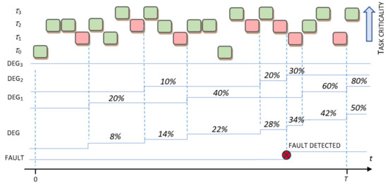
Figure 1.
Task execution scenario illustrating estimation of task and application-level performance degradations and system failure.
Table 2.
Task performance-model settings and execution properties in observed time interval.
The task model parameters given in Table 2 are adopted to illustrate the performance modeling of all three supported task types. As missing the deadline of a hard real-time task does not degrade system performance but causes immediate system failure, the weighting factor in the task performance model of such task type (), is set to 0. In the case of a firm task, , weighting factor is adjusted to 0.6, and the value of is adopted to imply that missing deadline in two succeeding task instances, in the selected time interval , may cause system failure. As missing the execution deadline of soft real time tasks cannot result in the system failures, modeling of such tasks requires us only to set a weighting factor. We adopted the value to quantify the impact of task misses on application performance.
Execution properties column from Table 2, matches the execution sequence presented in Figure 1. The execution properties include the information of total number of task instances expected to be executed in observation period, and the total number of instances with missed deadlines given as .
As given in Figure 1, missing a single deadline of task instance results in an increase of task-level degradation value by and application-level degradation of , whereas missing a deadline of task instance results in task and application level underperformances of and , respectively.
The simplified model for the estimation of task-level performance, where the task absolute deadline corresponds to the time instance of the succeeding event that triggers task execution, is compatible with the event-driven implementation model, where task-level performance is estimated upon the new event processing requested. Missing to finish the processing of previous events upon the occurrence of new events indicates the missing deadline condition and the corresponding performance degradation. Although not explicitly given, task-level performance estimation is therefore interchangeable with the event-based performance estimation, as processing of the single event may lead to the execution of the group of real-time tasks. In such implementation, performance modeling and the related parameters should be coupled with the events, whereas the processing of these events conforms to soft, firm, or hard criticality level.
3.3. Utilization Control Technique
Whereas the introduced performance metrics provide the outline for assessment of the application performance, the utilization control technique enables its control. Control of the application performance is supported through the created utilization control task described with the task model parameters . The setting of task model parameters is found from the adopted UCT settings, specified with the task priority and its utilization . The task execution time from the task model is found from expression , as the task period is equal to the observation period .
The aim of the utilization control is to provide at least utilization level of the introduced task by dynamically switching the priority of task between the two, and , priority levels. The value of is known a priory and is OS defined, whereas the value of is found from UCT settings.
The logic of utilization control (UC) that drives switching of UC task priorities is described as follows. During the observation period , the achieved utilization of the task is evaluated at the boundary of the selected task execution interval, e.g., tick interval or other adopted execution interval that allows fine-grained resolution of utilization tuning. Thus, the utilization of during the observation interval is achieved through the sequence of task executions with the total execution time of . The evaluation of total task utilization is performed following the simple criterion where the priority of the task is set to the selected priority level, if the current utilization of task is below the selected utilization level, otherwise task priority is adjusted to the to be executed within the following execution interval. Execution of UC task at the priority level may conform to the idle processing scenario, where arbitrary even-processing request may preempt the execution of UC task.
Additionally, execution of the task at the priority level with the total duration of may be given as a sequence of the task executions separated with the task executions at the priority. Implementing UCT to support such execution scenarios of UC tasks enables tasks with lower priorities at the ready-to-run state to be computed between the two succeeding task instances executed at higher priority level. Although the execution of higher priority tasks is not affected, and the total utilization of tasks remain the same, response time in of lower priority tasks may be enhanced. As the logic to follow this execution scenario is more complex, while the performance degradation level stays at the comparable level, to show up and discuss the effectiveness of UCT, we adopted a simplified form of UC task execution. The analysis of the several workload execution scenarios under different UCT settings is described in the rest of the section.
As the utilization of the original workload is below one, introduction of UC task results in rise of system utilization. Depending on the adopted UCT settings several workload execution scenarios are identified as follows:
The value of is the upper bound of the CPU utilization, e.g., labeled as utilization bound, that guarantees that all application tasks will meet their deadlines. As known from scheduling theory, the actual value of the utilization bound depends on the properties of the adopted scheduling policy [39,40] and the workload properties. According to the rate-monotonic analysis (RMA) as a theory underlying the static scheduling policy, utilization bound asymptotically approaches 69%, as the number of tasks in the workload reaches infinity. For the case studies analyzing the execution of pseudo-periodic tasks, RMA analysis has only theoretical implications as it addresses the scenario with the execution of periodical tasks.
For the system operation under case 1, the resulting application performance is not affected with the introduction of periodic utilization control tasks , as the total system utilization is below utilization bound. In contrast, power consumption can be considerably adjusted, e.g., increased or decreased, depending on the selected frequency scaling factor. Power management under such a scenario of system operation is exploited by voltage and frequency scaling techniques.
For the system operation under the condition defined as case 2, system power consumption is not significantly affected by changing the parameters . However, as operating above the utilization bound, some of low-priority task instances with the priorities might miss their deadline, resulting in the application underperformance.
Case 3, where the utilization is selected to result in overloaded system operation, system underperformance is expected, as low-priority task instances with the priority value above will mandatorily miss their deadlines. In such an execution scenario, the injection of idle processing with a task results in a controlled reduction of system power consumption with the relational increase in performance degradation. Selectivity of the presented technique is achieved through the adjusted priority level and the utilization value , as the task execution affects only the execution of application tasks with the priority values above . Thus, the execution of tasks with higher priorities are not affected regardless of the selected UC task utilization. However, the execution of lower priority tasks is affected proportionally to the selected utilization value.
To illustrate and discuss the application of the introduced control technique on real-time system operation, task scheduling, and trade-off management, the following use cases of workload execution under different UCT settings are evaluated.
The adopted workload is given in the form of the set of the tasks with the associated parameters, as given in Table 3.
Table 3.
Settings of workload model parameters.
To simplify the analysis, the utilization bound of is assumed. Because the adopted value for utilization bound, case 2 is removed from possible workload execution scenarios defined in (13). Additionally, as the execution case 1 corresponds to the workload execution without deadline misses, and therefore without performance degradation, this scenario is also excluded from execution use cases presented in Figure 2.
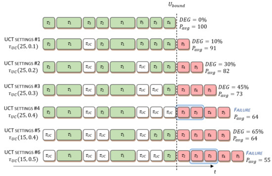
Figure 2.
Workload execution use cases under different UCT settings. Red boxes indicate task instances with missed deadlines, and green boxes represent correctly executed instances. White boxes represent the instances of the UCT task executions.
Figure 2 illustrates several workload execution scenarios under the different UCT parameter settings that conform to the overloaded system operation defined with case 3. UCT settings are specified at the left side of the execution pattern, illustrated with green, white, and red boxes. As the applying UCT impacts both application performance and the power consumption, resulting values are presented at the right side of the execution pattern. Indications of the failure condition, coupled with the execution of hard and firm real-time tasks, are also given.
The adopted value of average power consumption during idle processing, e.g., during UC task execution, is .
The upper sequence of task instances corresponds to the execution of the original workload without the UC task. Under the UCT settings #1, the priority setup of the UC task ensures its execution in the observed period. Consequently, the application degrades its performance because the instance of the task , as the instance of the task with the lowest priority, misses its deadline. Further increase in the utilization of the UC task, under UCT settings #2 and #3, consumes additional time span in the observed time interval, causing additional task instances with the lower priorities to miss their deadlines. UCT settings #4 enforce that the UC task consumes all the remaining time intervals executed at the priority level above 25. This results in operational fault caused by fault condition specified by task model (), as both task instances of the task missed their deadline. In contrast, increasing the priority level of UC task, according to the UCT settings #5, opens an additional time slot for degrading application performance. This time slot corresponds to the time intervals consumed for the execution of task instances. Unfortunately, further increase in the utilization of UC task, under UCT settings #6, leads to the fatal system fault caused by failure in task execution.
Although introduced for a uniprocessor platform, applicability of the approach is not limited in the case of multiprocessor systems. The rest of the section presents the discussion on how the proposed approach can be generalized to other task models in future work, e.g., to semi-partitioned scheduling [46] or to parallel task models [47,48].
Depending on the overlaying power management strategy, load, or power balancing requirements, a UC task may be statically partitioned and independently controlled or be subject to a controlled and limited migration across multiple processors during its execution. Partitioned approach resembles a uniprocessor case where each UC task is running on an associated processor depending on its local UCT settings. In contrast, multiprocessor real-time systems with the semi-partitioned scheduling are offering additional flexibility for the implementation of UCT. Regardless of UCT, such systems are offering more optimal run-time behavior, compared with static partitioning and global scheduling approaches under the dynamic workloads found in the multimedia, robotics, cloud, and fog computing applications. Semi-partitioned approach of UCT implementation may follow execution of a UC task upon a semi-partitioned reservation whose execution budget is split across multiple processors [46]. In such a scenario, after the UC task exhausts the reserved budget on the current processor, its execution migrates to another processor where it will be served by corresponding tail reservation. Sequential UC task models may be extended to parallel task models that conform to the execution on multi-core processor platforms. Parallel task models of a UC task may consider a set of synchronous parallel tasks, where each task is represented as a sequence of segments containing parallel threads that synchronize at the end of the segment [47]. Analogous to the use case given in Figure 2, task segments conform to the presented task instances, whereas the execution requirements of each parallel thread are tuned according to the UCT settings. Adoption of a UC task model to be compliant with Directed Acyclic Graph (DAG) task model, as an even more general model for parallel tasks, may further extend its applicability on heterogeneous distributed processor systems. As given in [48], combining such representation of a UC task combined with the energy-aware DAG scheduling makes UCT suitable for heterogeneous processors that can run on discrete operating voltages, extending its applicability on high performance DSP platforms, in image processing, multimedia, and wireless security applications.
4. Results and Discussion
The parametric analysis of the effectiveness of UCT in the context of power–performance trade-offs is investigated in the simulation environment for several workload execution scenarios. Model parameters of the workload given in the form of periodic tasks set with the assumed implicit deadlines, are given in Table 4.
Table 4.
Settings of workload model parameters.
The adopted power model presumes uniform task-level consumption specified with and . Consumption parameters of utilization control tasks are set to and , as they are related to idle processing. Parameters and in relation (3) that define the CPU voltage-frequency relationship are selected as and .
Weight factors for performance modeling are calculated from used task-priorities as:
where the lowest task priority level is given as , and , as the weight factor of tasks with a hard level of criticality is set to zero. Although the degradation weight factor of individual tasks can be assigned in various ways, we adopted Relationship (14), so the weight factor is inversely proportional to assigned task priorities. The parameters for firm tasks are selected to conform with the situation where 50% of firm tasks in sequence are missing their deadline in the observation interval. The value of observation interval is evaluated based on the Relation (5) as .
The expression for estimating an application-level performance degradation, from Equation (11), is adopted in the form of weighted sum of individual task degradations as:
where degradation of firm and soft real-time tasks, e.g., values of , is estimated according to Equation (12). As the sum of all weight factors is selected to be 1, according to the Relations (14) and (15), application-level degradation is bounded at 100%.
4.1. Effectiveness of UCT
The following analysis illustrates the trade-off potential of the introduced utilization control technique applicable in the scenarios where the voltage and frequency scaling are not available or there are significant drawbacks regarding its frequent use. Because in such scenarios the frequency scaling value is fixed, the trade-off control is achieved solely through the control of parameters.
Performance degradation and normalized average power consumption for the scenario of the overloaded execution of workload defined in Table 4, under different UCT parameter settings, are presented in Figure 3, where represents average system-level power consumption for system operation during the observation period under the nominal frequency and voltage settings.
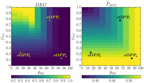
Figure 3.
Heat map graph of application performance (left) and power (right) metrics in the 2D space of UCT control parameters .
Results presented in Figure 3 demonstrate the effectiveness of UCT in 2D UCT parameter space defined with 2-tuple . Presented results are evaluated for fixed settings that correspond to CPU frequency of . As both groups of parameters, settings in voltage-frequency domain and UCT settings in utilization domain, affect the system behavior in power-performance domain, they are all considered as an extended set of system-level parameters for tuning power–performance trade-off. Further on, this expanded set of application controllable parameters is considered as extended operating point parameters denoted as .
As shown in Figure 3, control of UCT parameters enables variation of application execution properties in the power and performance domain of up to 25% and 80%, respectively. Analyzing the heat map graph on the left-hand side, one could notice that application performance degrades from 17.3% at the right side toward 100% at the top-left side of the heat map. The area at the right side of the heat map graph corresponds to the UCT settings where UC task priority is set at the levels that may affect only the operation of soft real-time tasks resulting in insignificant performance degradation. However, UCT settings where UC task priority and utilization are affecting the operation of a firm real-time task, as found in the top-left side of the heat map graph, results in significant performance losses, noticeable as yellow-colored areas on the heat map graph. Similar analysis may be performed on the heat map graph presented on the right-hand side in Figure 3. It is noticeable that heat distribution resembles a contrast of the heat map graph presented on the left-hand side, confirming the trade-off potential in driving particular embedded applications in the power-performance domain.
To demonstrate the trade-off potential of the utilization control technique for fine-grained tuning of application execution properties, several s are selected as presented in Table 5. The resulting power and performance properties of workload execution are also given.
Table 5.
Properties of the system operation for selected s from Figure 3.
Generalized observation given in the analysis of Figure 3 are further evaluated in Table 5. As noticeable from Table 5, with varying parameters the system-level average power consumption and application underperformance change in the opposite direction, confirming the foundation for power–performance trade-offs. Compared to the traditional technique of voltage and frequency scaling, which selects the system operating point in the 1D space, introduction of additional parameters extends the space of system operating point parameters to 3D. Thus, from the context of optimizing power efficiency, UCT can be considered as an extension of native DVFS approach and vice versa. By combining DVFS and UCT, operating point parameter space is expanded, although tuning of parameters can be separately applied for power and performance management at the application-level.
The analysis presented in the rest of the section illustrates the joint potential of utilization control and DVFS approaches, denoted as UC-DVFS approach, driving system operation even beyond the utilization bound. The investigation also reveals the trade-off area in the power–performance domain established by extension of operating point parameters through UCT.
4.2. Exploring the Limits of UC-DVFS Approach
The effectiveness of the proposed UC-DVFS approach for the management of the power–performance trade-off in different workload execution scenarios is presented in Figure 4. The parameters of the workload used in simulations are defined in Table 4. The execution scenarios cover different settings where frequency was scaled in the range , was changed in the range from to , and was varied in the range from 0 to 1. Red line and light and dark blue areas in Figure 4 represent points in the power–performance domain for different and parameters settings, where the system operates without faults.
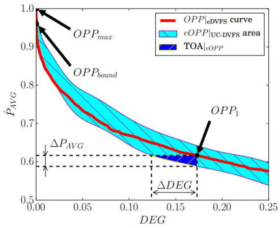
Figure 4.
System operating points in power-performance domain in and parameters space.
The curve, given with the red line, shows power and performance properties of the system operation under the adopted frequency range. As the workload execution at assumes system operation below the utilization bound, the presented analysis included both execution cases defined in (13), e.g., case 1 and case 3. The properties of the system operation under different 3D parameter settings, defined with , are visualized with a light blue area. As observable from Figure 4, introduction of additional parameters, e.g., and , expands the potential for the management of system operation in the power-performance domain.
To discuss the outcomes of the conducted analysis, three characteristic system operating points are identified as , , and . The corresponding power and performance properties of the system operation under selected system s is given in Table 6, where is initial operating point at , e.g., at , where the total CPU utilization is below utilization bound . The is the system operating point, where the frequency scaling factor () is adjusted to scale the workload utilization to its boundary value. This operating point is considered as a boundary between the system operation with and without degraded performance. The value of is chosen as a representative system operating point during overloaded system operation selected in 1D operating parameters space at .
Table 6.
Properties of the system operation for operating points defined in Figure 4.
In the context of standard inter-task power management techniques, the system operated in the range between and illustrates the potential of standard DVFS under the adopted workload model. Adjusting the frequency scaling factor to the value of 0.77 enables energy savings of 3.3% compared with the system operation under nominal frequency settings, e.g., . The introduced metrics for quantifying system performance enable observable system operation even beyond , in the region of overloaded system operation. System operation in this region with degraded application performance, marked with a red line in Figure 4, enables significantly higher power savings compared with the standard DVFS operating up to the . Further workload execution, under the frequency scaling ranged from 0.77 to 0.12, enable significant power savings, reaching a level of at . Utilization of standard DVFS technique in the region beyond and toward is denoted as extended DVFS, or eDVFS in Figure 4.
Individual contribution of the UCT on the power efficiency is further identified through the detailed analysis of trade-off area (TOA), which is shown in Figure 4 and Figure 5 in expanded form. As discussed previously, a combined UC-DVFS approach enables fine-grained power performance trade-off through the control of in the 3D-space of system parameters. Compared with eDVFS, further extension of system operating parameters introduces potential for more efficient application execution. To anticipate the contribution of the UCT, properties of system execution at selected operating points are evaluated and compared with the system operation at .
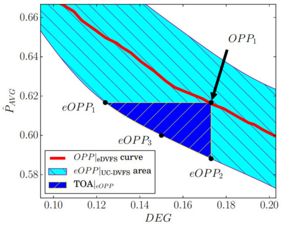
Figure 5.
Extended operating points in the trade-off area for the selected from Figure 4.
As illustrated in Figure 5 and quantified in Table 7, different s can be selected to lower performance degradation (), to lower power consumption (), or to enable enhancements in both domains (). Adjustment of operating point parameters enables relative improvement of application performance at the of 28.3%, compared with the system operation at under the identical power budget. In contrast, operation at enables relative decrease of 4.5% in power consumption under the same performance level as in .
Table 7.
Properties of the system operation at and characteristic s in the TOA.
To make a point from previous analysis, extension of operating point parameters from 1D to 3D parameter space enables fine grained control and more efficient system operation in both power and performance domains.
The further analysis exploits the trade-off potential for optimizing system behavior in the power–performance domain. The UC-DVFS provides an implicit link between the extended operating point defined in the 3D space of system parameters and the operating point in the power–performance domain given with the pair of values . This link allows for the introduction of different management relationships that quantify the trade-off between and .
In the remainder of the paper, we analyze the optimized system operation under the different optimization criteria extracted from simple trade-off management relation () given in the form of linear Equation (16). Although different more complex relationships may be more appropriate for particular applications, the simplified form of is adopted, as the selection of is not affecting the optimization process but rather the optimization outcome.
The introduces parameter used to set the goal of trade-off management toward more efficient system operation under the required performance level or available power budget:
By setting the value of , different settings in 3D parameter space are found to optimize, e.g., minimize the value of the relation. The results shown in Figure 6 provide insight into the influence of setting different trade-off criteria, obtained by varying parameter , on optimal system behavior.
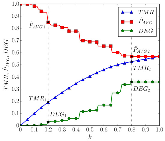
Figure 6.
Data points represent optimized power and performance behavior of system operation under different trade-off management relations varied by the parameter .
Regions of optimal system operation under the boundary cases of TMR defined with and elevates the impact of system performance or system power consumption on the selection of . The boundary cases conform to the adopted trade-off management relation and the workload model parameters and are selected based on the observed properties of and curves from Figure 6. As noticeable from Figure 6, optimal system behavior under parameter settings , results in significant power savings (15% at ) with minimal degradation of performance level (near 3% at ), where system operates near the utilization bound from Figure 4. Analyzing system behavior under reveals that the system reaches its limits in minimizing system power consumption (power savings of 43% at ), at the same time, maximally degrading application performance (approx. 36% at ) without system failures. As obvious from Figure 6, optimal settings depend on the selected criteria, actual system performance, as well as power consumption. The following paragraph discusses limitations and challenges regarding the application of presented methodology.
To be applied in the physical world, where power and performance models are not a priori known, regardless of the selected criteria, an tracking algorithm may be needed to provide the optimal system operation in the power–performance domain. Additionally, the proposed performance model may not fit the application needs and criticality architecture of the workload. The proposed coarse-grained approach for estimating degradation level of the workload execution is result of the intention to omit the requirements for measuring or estimating timing properties of the task execution. Thus, the presented performance model simplifies its implementation, and, at the same time, provides the support for event-driven performance estimation. From the power consumption point of view, the application of the proposed static power model is limited to the simulation of system behavior and presentation of the proposed power management approach. In real-world scenarios, the power consumption may require more complex dynamic modeling, or the estimation obtained from direct power consumption measurements.
5. Conclusions
In this paper, we presented the methodology that allows fine-grained power–performance trade-off by introducing metrics for estimating application performance and by extending the set of application-level operating point parameters for performance control. The extension of operating point parameters resulted from the introduction of the technique for fine-grained management of power–performance trade-offs. The introduced utilization control technique as a part of the proposed methodology enables selective degradation of the application tasks at the arbitrary criticality level, without affecting the execution of safety-critical features. The evaluation of the proposed techniques confirmed more energy efficient system operation in the power–performance domain compared with the traditional DVFS approach. Furthermore, the presented methodology provides the background for the design of more sophisticated power and energy management solutions utilizing the effectiveness of UCT and combined UC-DVFS approaches for driving the real-time embedded systems even beyond the safe boundaries. The main original contribution of the proposed methodology is in making the bound between the power and performance domains, providing the background for associated trade-offs, and the technique that enables control of trade-offs through the simple upgrade of the traditional RTOS with static priority-based scheduling.
Multi-level variants of UCT, as well the implementation of the presented methodology in the RTOS environment as a framework that enables integration of arbitrary algorithms for the control of operating point parameters and the selection of appropriate optimization criteria that fits the application needs, will be part of future work.
Author Contributions
Conceptualization, I.P. and S.J.; software, S.J.; validation, I.P. and S.J.; formal analysis, I.P. and S.J.; investigation, I.P. and S.J.; resources, S.J.; data curation, I.P. and S.J.; writing—original draft preparation, I.P. and S.J.; writing—review and editing, I.P. and S.J.; visualization, I.P. and S.J.; supervision, I.P.; project administration, I.P.; funding acquisition, I.P. and S.J. All authors have read and agreed to the published version of the manuscript.
Funding
This research was funded by the Ministry of Education, Science and Technological Development, Republic of Serbia through Grant Agreement with University of Belgrade-School of Electrical Engineering No: 451-03-9/2021-14/200103.
Acknowledgments
The authors gratefully acknowledge the financial support from the Ministry of Education, Science, and Technological Development of the Republic of Serbia.
Conflicts of Interest
The authors declare no conflict of interest.
Abbreviations
| IoT | Internet of Things |
| WSN | Wireless Sensor Network |
| IC | Integrated Circuit |
| OS | Operating System |
| RTOS | Real Time Operating System |
| UCT | Utilization Control Technique |
| UC | Utilization Control |
| DAG | Directed Acyclic Graph |
| UC-DVFS | Utilization Control with Dynamic Voltage and Frequency Scaling |
| DVFS | Dynamic Voltage and Frequency Scaling |
| SPM | Static Power Management |
| DPM | Dynamic Power Management |
| PM | Power Management |
| HPC | High-Performance Computing |
| MPI | Message Passing Interface |
| CPU | Central Processing Unit |
| EDF | Earliest Deadline First |
| MCS | Mixed Criticality Systems |
| EDP | Energy Delay Product |
| HW | Hardware |
| SW | Software |
| WCET | Worst Case Execution Time |
| OPP | Operating Point Parameters |
| LCM | Least Common Multiple |
| RMA | Rate Monotonic Analysis |
| 3D | Three Dimensions |
| eOPP | Extended Operating Point Parameters |
| eDVFS | Extended Dynamic Voltage and Frequency Scaling |
| TOA | Trade-off Area |
| TMR | Trade-off Management Relation |
Appendix A. List of Symbols
| Workload given as a set of application tasks | |
| Task model parameters | |
| Task priority value where higher priority value indicates lower task priority level | |
| Task period as a minimal interval between the arrival of two succeeding task instances | |
| Worst case task execution of task instance | |
| Task relative deadline | |
| Idle task priority as the lowest task priority level | |
| Frequency scaling factor given as | |
| Nominal CPU frequency settings | |
| Voltage scaling factor given as | |
| Nominal microprocessor supply voltage settings | |
| System-level power consumption during the execution of the task under the given frequency and voltage scaling factor settings | |
| Power consumption of microprocessor IC under given voltage and frequency scaling and during the execution of the task | |
| Overall power consumption of all system components, whose operation is not affected by voltage and frequency scaling, during the execution of task | |
| Power consumption of microprocessor IC under nominal voltage and frequency settings and during the execution of the task | |
| Operating point under given frequency scaling factor settings | |
| System-level power consumption during the execution of the task under the given frequency scaling factor settings | |
| Observation period for workload Γ found as least common multiple of task periods | |
| Utilization of task under given frequency scaling factor settings | |
| Maximum application utilization value during the observation period under given frequency scaling factor settings | |
| Number of task instances that arrive for execution during the observation period | |
| System-level average power consumption during the observation period | |
| Average power consumption during the idle processing under given frequency scaling factor settings | |
| Application-level performance degradation | |
| Task-level performance degradation | |
| Degradation weighting factor for task | |
| Number of task instances that missed their deadline in the observation period | |
| Number of firm-criticality task consecutive instances where missing their deadlines leads to complete system failure | |
| Task criticality assignment, where corresponds to soft, firm, and hard task criticality levels | |
| Priority assignment for utilization control task | |
| Utilization assignment for utilization control task | |
| Utilization bound, that guarantees that all application tasks will meet their deadlines | |
| Normalized system-level average power consumption during the observation period found as | |
| Average system-level power consumption for system operation during the observation period under the nominal frequency and voltage settings | |
| Extended set of operating point parameters | |
| System operating point in power-performance domain |
References
- Hassan, R.; Qamar, F.; Hasan, M.K.; Aman, A.H.M.; Ahmed, A.S. Internet of Things and Its Applications: A Comprehensive Survey. Symmetry 2020, 12, 1674. [Google Scholar] [CrossRef]
- Tanweer, A. A Reliable Communication Framework and Its Use in Internet of Things (IoT). Int. J. Sci. Res. Comput. Sci. Eng. Inf. Technol. 2018, 5, 450–456. [Google Scholar]
- Etinski, M.; Corbalan, J.; Labarta, J.; Valero, M. Understanding the future of energy performance trade-off via DVFS in HPC environments. J. Parallel Distrib. Comput. 2012, 72, 579–590. [Google Scholar] [CrossRef]
- Thakkar, A.; Chaudhari, K.; Shah, M. A Comprehensive Survey on Energy-Efficient Power Management Techniques. Procedia Comput. Sci. 2020, 167, 1189–1199. [Google Scholar] [CrossRef]
- Chetto, M.; El Ghor, H. Scheduling and power management in energy harvesting computing systems with real-time constraints. J. Syst. Arch. 2019, 98, 243–248. [Google Scholar] [CrossRef]
- Wu, H.; Chen, C.; Weng, K. An Energy-Efficient Strategy for Microcontrollers. Appl. Sci. 2021, 11, 2581. [Google Scholar] [CrossRef]
- Chéour, R.; Jmal, M.W.; Khriji, S.; El Houssaini, D.; Trigona, C.; Abid, M.; Kanoun, O. Towards Hybrid Energy-Efficient Power Management in Wireless Sensor Networks. Sensors 2022, 22, 301. [Google Scholar] [CrossRef]
- Bambagini, M.; Marinoni, M.; Aydin, H.; Buttazzo, G. Energy-Aware Scheduling for Real-Time Systems: A Survey. Trans. Embed. Comput. Syst. 2016, 15, 7. [Google Scholar] [CrossRef]
- Kim, Y.G.; Kong, J.; Chung, S.W. A survey on recent OS-level energy management techniques for mobile processing units. IEEE Trans. Parallel Distrib. Syst. 2018, 29, 2388–2401. [Google Scholar] [CrossRef]
- Moyer, B. Low-power design for embedded processors. Proc. IEEE Inst. Electr. Electron. Eng. 2001, 89, 1576–1589. [Google Scholar] [CrossRef]
- Baruah, S.; Bonifaci, V.; D’Angelo, G.; Li, H.; Marchetti-Spaccamela, A.; van der Ster, S.; Stougie, L. The Preemptive Uniprocessor Scheduling of Mixed-Criticality Implicit-Deadline Sporadic Task Systems. In Proceedings of the 24th Euromicro Conference on Real-Time Systems (ECRTS), Pisa, Italy, 10–13 July 2012. [Google Scholar] [CrossRef]
- Vestal, S. Preemptive scheduling of multi-criticality systems with varying degrees of execution time assurance. In Proceedings of the 28th IEEE International Real-Time Systems Symposium (RTSS 2007), Tucson, AZ, USA, 3–6 December 2007; pp. 239–243. [Google Scholar] [CrossRef]
- Ma, W.; Cheng, Q.; Gao, Y.; Xu, L.; Yu, N. An Ultra-Low-Power Embedded Processor with Variable Micro-Architecture. Micromachines 2021, 12, 292. [Google Scholar] [CrossRef] [PubMed]
- Legout, V.; Jan, M.; Pautet, L. Mixed-criticality multiprocessor real-time systems: Energy consumption vs deadline misses. In Proceedings of the First Workshop on Real-Time Mixed Criticality Systems (ReTiMiCS), Taipei, Taiwan, 19–21 August 2013; Available online: https://hal-imt.archives-ouvertes.fr/hal-00922522 (accessed on 29 April 2022).
- Fadlelseed, S.; Kirner, R.; Menon, C. ATMP-CA: Optimising Mixed-Criticality Systems Considering Criticality Arithmetic. Electronics 2021, 10, 1352. [Google Scholar] [CrossRef]
- Guo, Z.; Yang, K.; Vaidhun, S.; Arefin, S.; Das, S.K.; Xiong, H. Uniprocessor Mixed-Criticality Scheduling with Graceful Degradation by Completion Rate. In Proceedings of the IEEE Real-Time Systems Symposium (RTSS), Nashville, TN, USA, 12–14 December 2018; pp. 373–383. [Google Scholar] [CrossRef]
- Laplante, P.A. Real-Time Systems Design and Analysis, 3rd ed.; Stamatios, V.K., Ed.; John Wiley & Sons: New York, NY, USA, 2004; ISBN 0-471-22855-9. [Google Scholar]
- Shye, A.; Scholbrock, B.; Memik, G. Into the wild: Studying real user activity patterns to guide power optimizations for mobile architectures. In Proceedings of the 42nd Annual IEEE/ACM International Symposium on Microarchitecture, New York, NY, USA, 12–16 December 2009; pp. 168–178. [Google Scholar] [CrossRef]
- Chen, Y.-L.; Chang, M.-F.; Yu, C.-W.; Chen, X.-Z.; Liang, W.-Y. Learning-Directed Dynamic Voltage and Frequency Scaling Scheme with Adjustable Performance for Single-Core and Multi-Core Embedded and Mobile Systems. Sensors 2018, 18, 3068. [Google Scholar] [CrossRef]
- Calore, E.; Gabbana, A.; Schifano, S.F.; Tripiccione, R. Software and DVFS Tuning for Performance and Energy-Efficiency on Intel KNL Processors. J. Low Power Electron. Appl. 2018, 8, 18. [Google Scholar] [CrossRef]
- Xu, R.; Mosse, D.; Melhem, R. Minimizing Expected Energy Consumption in Real-time Systems through Dynamic Voltage Scaling. ACM Trans. Comput. Syst. 2007, 25, 9. [Google Scholar] [CrossRef]
- Liu, S.; Qiu, Q.; Wu, Q. Energy Aware Dynamic Voltage and Frequency Selection for Real-time Systems with Energy Harvesting. In Proceedings of the Design, Automation and Test in Europe, (DATE ’08), Munich, Germany, 10–14 March 2008; pp. 236–241. [Google Scholar] [CrossRef]
- Xu, H.; Li, R.; Zeng, L.; Li, K.; Pan, C. Energy-efficient scheduling with reliability guarantee in embedded real-time systems. Sustain. Comput. Inform. Syst. 2018, 18, 137–148. [Google Scholar] [CrossRef]
- Haririan, P. DVFS and Its Architectural Simulation Models for Improving Energy Efficiency of Complex Embedded Systems in Early Design Phase. Computers 2020, 9, 2. [Google Scholar] [CrossRef]
- Chéour, R.; Khriji, S.; Götz, M.; Abid, M.; Kanoun, O. Accurate Dynamic Voltage and Frequency Scaling Measurement for Low-Power Microcontrollors in Wireless Sensor Networks. Microelectron. J. 2020, 105, 104874. [Google Scholar] [CrossRef]
- Aydin, H.; Melhem, R.; Mosse, D.; Mejia-Alvarez, P. Power-aware scheduling for periodic real-time tasks. IEEE Trans. Comput. 2004, 53, 584–600. [Google Scholar] [CrossRef]
- Zhang, Y.; Li, H. Energy aware mixed tasks scheduling in real-time systems. Sustain. Comput. Inform. Syst. 2019, 23, 38–48. [Google Scholar] [CrossRef]
- Moser, C.; Brunelli, D.; Thiele, L.; Benini, L. Lazy Scheduling for Energy Harvesting Sensor Nodes. In Proceedings of the Working Conference on Distributed and Parallel Embedded Systems (DIPES 2006), Braga, Portugal, 11–13 October 2006; pp. 125–134. [Google Scholar] [CrossRef]
- Severini, M.; Squartini, S.; Piazza, F. Energy-aware lazy scheduling algorithm for energy-harvesting sensor nodes. Neural Comput. Appl. 2013, 23, 1899–1908. [Google Scholar] [CrossRef]
- Kim, Y.; Lee, K.-S.; Lee, C.-G. Energy Efficient Real-Time Scheduling Using DPM on Mobile Sensors with a Uniform Multi-Cores. Sensors 2017, 17, 2906. [Google Scholar] [CrossRef] [PubMed]
- Marchand, A.; Chetto, M. Dynamic scheduling of periodic skippable tasks in an overloaded real-time system. In Proceedings of the International Conference on Computer Systems and Applications (IEEE/ACS), Doha, Qatar, 31 March–4 April 2008; pp. 456–464. [Google Scholar] [CrossRef]
- Chéour, R.; Jmal, M.; Kanoun, O.; Abid, M. Evaluation of Simulators Tools and Power-Aware Scheduling Model for Wireless Sensor Networks. IET Compute. Dig. Tech. 2017, 11, 173–182. [Google Scholar] [CrossRef]
- Mittal, S. A Survey of Techniques for Approximate Computing. ACM Comput. Surv. 2016, 48, 62. [Google Scholar] [CrossRef]
- Liu, J.W.S.; Shih, W.-K.; Lin, K.-J.; Bettati, R.; Chung, J.-Y. Imprecise computations. Proc. IEEE 1994, 82, 83–94. [Google Scholar] [CrossRef]
- Wiedenhoft, G.R.; Frhlich, A.A. Using Imprecise Computation Techniques for Power Management in Real-Time Embedded Systems. In Proceedings of the Working Conference on Distributed and Parallel Embedded Systems (DIPES 2008), Milano, Italy, 7–10 September 2008; pp. 121–130. [Google Scholar] [CrossRef]
- Hua, S.; Qu, G.; Bhattacharyya, S.S. An energy reduction technique for multimedia application with tolerance to deadline misses. In Proceedings of the Design Automation Conference (IEEE Cat. No.03CH37451), Anaheim, CA, USA, 2–6 June 2003; pp. 131–136. [Google Scholar] [CrossRef]
- Gotz, M.; Khriji, S.; Chéour, R.; Arief, W.; Kanoun, O. Benchmarking based Investigation on Energy Efficiency of Low-Power Microcontrollers. IEEE Trans. Instrum. Meas. 2020, 69, 7505–7512. [Google Scholar] [CrossRef]
- Broekaert, F.; Fritsch, A.; Sa, L.; Tverdyshev, S. Towards power-efficient mixed-critical systems. In Proceedings of the 9th annual workshop on Operating Systems Platforms for Embedded Real-Time Applications (OSPERT), Paris, France, 10–12 July 2013; pp. 31–35. Available online: http://citeseerx.ist.psu.edu/viewdoc/download?doi=10.1.1.385.4299&rep=rep1&type=pdf#page=31 (accessed on 29 April 2022).
- Sha, L.; Abdelzaher, T.; Arzen, K.-E.; Cervin, A.; Baker, T.; Burns, A.; Buttazzo, G.; Caccamo, M.; Lehoczky, J.; Mok, A.K. Real Time Scheduling Theory: A Historical Perspective. Real-Time Syst. 2004, 28, 101–155. [Google Scholar] [CrossRef]
- Liu, C.L.; Layland, J.W. Scheduling Algorithms for Multiprogramming in a Hard-Real Time Environment. J. ACM 1973, 20, 46–61. [Google Scholar] [CrossRef]
- Ali, I.; Jo, Y.-I.; Lee, S.; Lee, W.Y.; Kim, K.H. Reducing Dynamic Power Consumption in Mixed-Critical Real-Time Systems. Appl. Sci. 2020, 10, 7256. [Google Scholar] [CrossRef]
- Maghsoud, Z.; Noori, H.; Mozaffari, S.P. PEPS: Predictive energy-efficient parallel scheduler for multi-core processors. J. Supercomput. 2021, 77, 6566–6585. [Google Scholar] [CrossRef]
- Ramesh, U.B.K.; Sentilles, S.; Crnkovic, I. Energy management in embedded systems: Towards a taxonomy. In Proceedings of the First International Workshop on Green and Sustainable Software (GREENS), Zurich, Switzerland, 3 June 2012; pp. 41–44. [Google Scholar] [CrossRef]
- Shailesh, T.; Nayak, A.; Prasad, D. An UML Based Performance Evaluation of Real-Time Systems Using Timed Petri Net. Computers 2020, 9, 94. [Google Scholar] [CrossRef]
- Silva-de-Souza, W.; Iranfar, A.; Bráulio, A.; Zapater, M.; Xavier-de-Souza, S.; Olcoz, K.; Atienza, D. Containergy—A Container-Based Energy and Performance Profiling Tool for Next Generation Workloads. Energies 2020, 13, 2162. [Google Scholar] [CrossRef]
- Casini, D.; Biondi, A.; Buttazzo, G. Task Splitting and Load Balancing of Dynamic Real-Time Workloads for Semi-Partitioned EDF. IEEE Trans. Comput. 2020, 70, 2168–2181. [Google Scholar] [CrossRef]
- Saifullah, A.; Agrawal, K.; Lu, C.; Gill, C. Multi-core real-time scheduling for generalized parallel task models. In Proceedings of the IEEE 32nd Real-Time Systems Symposium (RTSS), Vienna, Austria, 29 November–2 December 2011; pp. 217–226. [Google Scholar] [CrossRef]
- Baskiyar, S.; Abdel-Kader, R. Energy aware DAG scheduling on heterogeneous systems. Cluster Comput. 2010, 13, 373–383. [Google Scholar] [CrossRef]


Publisher’s Note: MDPI stays neutral with regard to jurisdictional claims in published maps and institutional affiliations. |
© 2022 by the authors. Licensee MDPI, Basel, Switzerland. This article is an open access article distributed under the terms and conditions of the Creative Commons Attribution (CC BY) license (https://creativecommons.org/licenses/by/4.0/).