3.1. Notation and Problem Definition
In accordance with the notations that are most often used, we denote sets as calligraphic fonts (e.g., ) and vectors as bold lowercase letters (e.g., ). Scalars are represented by lowercase letters (e.g., l). We refer to matrices as bold uppercase letters (e.g., ), and indicates the ith row in .
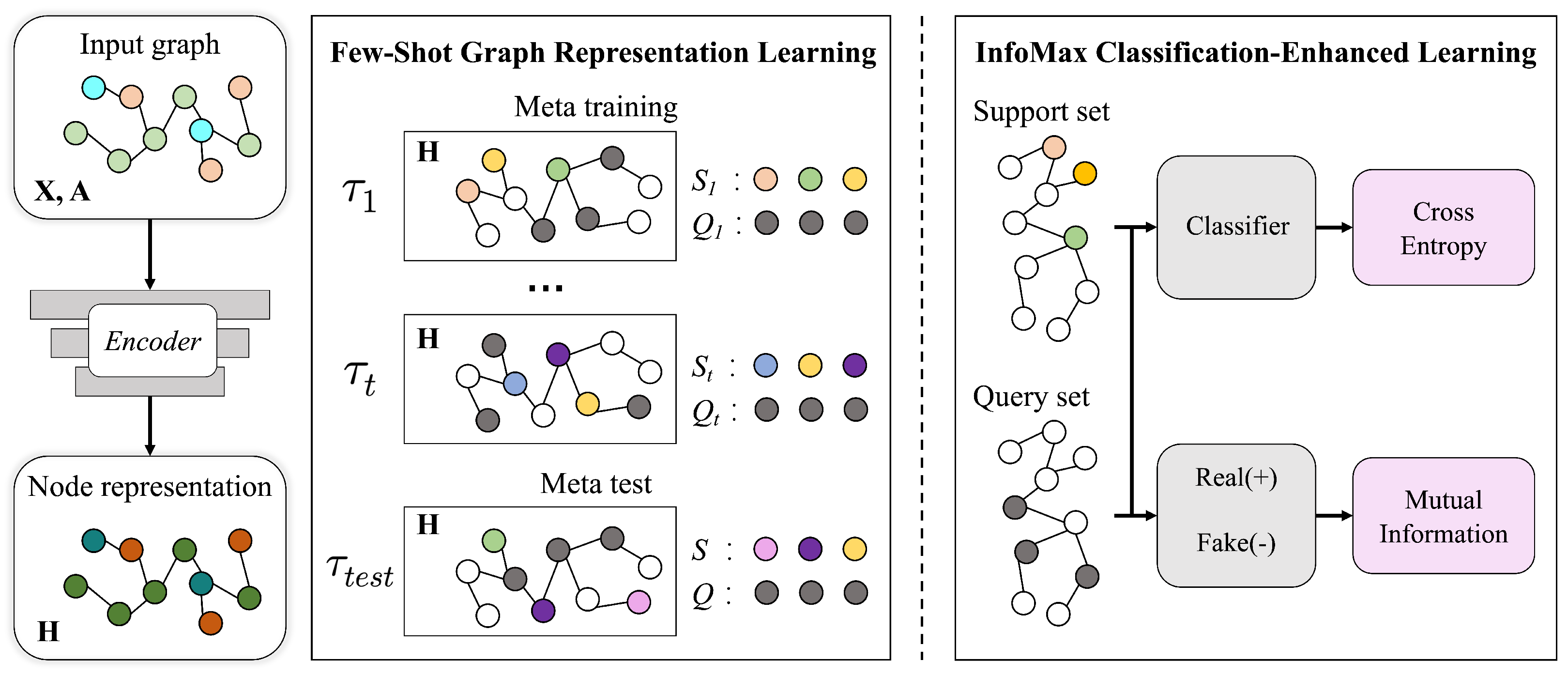
An undirected attributed graph is referred to as a quadruple , where is the node set, n denotes the total number of nodes, is the edge set, represents the asymmetric adjacency matrix that represents the graph structure, and means node and node are connected by an edge. is the attributed feature matrix, a row vector represents a node’s () characteristic information, and its dimension is d.
Problem Definition: With a direct attributed graph , we are looking forward to learning a network encoder and a classifier from a limited number of labeled nodes that can be adapted to a disjoint set of new classes to predict nodes’ labels. In most cases, there are just a few nodes for which the labels may be provided. Formally, following the few-shot learning (FSL) settings, the nodes in training set contain C classes, and the nodes in the disjoint testing set contain N unseen classes. In , if each class has K nodes that are labeled and make up the support set , the task is referred to as an N-way K-shot node classification task, and K is usually a relatively small number, such as one, three, or five. Our purpose is finding and training a suitable network encoder that can obtain good node representations and make accurate predictions about the labels of the remaining unlabeled nodes (also called the query set ). Thus, the meta-learning problem on the graph is addressed as a few-shot node classification problem, and the key lies in how to extract knowledge that can be transferred from the training data to testing data that have not been seen before.
3.2. Few-Shot Graph Representation Learning
The methodology for addressing the problem of few-shot node classification largely depends on the graph representation learning module as its core component. In designing the framework, we made sure to take into account two difficult research topics:
- •
How to conduct meta-learning on graph structure data and how to extract information that can be transferred from the training data to testing data when there are only a handful of labeled nodes available.
- •
How to make the most of the limited number of nodes that are available in the support set and restrict the query set to obtain informative and discriminative representations?
As can be seen in
Figure 1, we constructed a meta-learning structure that is based on the concept of episodic categorization. To be more specific, the training process is composed of a large number of meta-training tasks sampled from task distribution, which is denoted as
, and trained episodically. The training process mimics the actual testing setting to alleviate the distribution gap between training and testing. After studying a significant amount of different episodes, the knowledge in graph topology and feature distribution can be extracted and passed through each episode and then applied to unseen classes in meta-testing tasks.
In order to assure that there will be no differences between the training and the tests, each task used in the meta-training phase and the meta-testing phase came from the same task distribution and were formed as an N-way K-shot classification task . For every task , we used to represent the support set and used to represent the query set. contains nodes and their corresponding labels from N different classes. contains nodes taken from the rest of the N classes, and the unknown labels are the labels to be predicted. The true labels of the query set nodes are disguised throughout the training phase so that it may be more similar to the testing procedure, and the actual labels are used to compute and evaluate the training loss. After T meta-training tasks and optimization with a gradient descent, the model is convergent and may be used to make predictions for unknown query nodes in meta-testing tasks with unseen classes. By completing these meta-training tasks, the model is able to acquire information that is not only portable from one episode to the next but also may be generalized to be applied to meta-testing tasks.
With a given
N-way
K-shot task, we employed an encoder network to capture the graph topology information
and the nodes’ feature matrix
to obtain a node’s representation. Specifically, we stacked several GNN layers to convey a node to a low-dimensional vector
. The GNNs follow the
pipeline, where the
step aggregates a node’s neighboring information, and the
step compresses the node features from the local neighborhoods. After
l instances of
operations, each node
v’s multi-hop messages are passed, and ultimate node representation
is obtained for predicting its class label
. A GNN layer may be described in a formal way as follows, and
l is the layer number:
where
is the node embedding at layer
l that is updated with the
function based on this node’s representation and its neighborhood representation
at the upper layer and
is the neighborhood representation based on
v’s neighborhood set
and the
function. The
operation can be any form of information aggregator, such as
,
,
, and the
function can be
,
or others. With the different choices of
and
functions, there is a series of implementations [
5,
10,
28]. We stacked
L instances of GNN layers above these two operations to build the graph encoder and obtain the node representations that may be used in the output layer for the purpose of node categorization. For simplicity, we denote the graph encoder as
and the graph encoder’s output matrix as
.
ś
ith row element, denoted as
, represents the ultimate node representation of node
.
3.3. InfoMax Classification-Enhanced Learning
After obtaining the node representations, we could perform classification and evaluate the model based on the misclassification rate. However, when it comes to learning in a few-shot task, the labeled nodes of the support set are limited to a small number, and the unlabeled query set nodes’ number is not fixed. We needed to make the most use of the scanty labels to train a task-specific classifier for unlabeled nodes and also make sure the query set nodes kept a similar feature distribution to the support set nodes. Thus, we propose InfoMax classification-enhanced learning. In a few-shot task, we first train a task-specific classifier with support set nodes and then restrict the query set nodes to have similar feature distribution to the support set nodes with mutual information maximization. By doing so, we enhance the accuracy of the node classification while simultaneously training the network encoder to learn the maximum comparable feature representation for the same class of nodes as before.
Class-Specific Classifier: We used support set nodes and their labels to train a task-specific classifier. The following is the definition of the classifier:
where
denotes the
ith node representation of
K nodes that belong to one of the
N different classes that make up the support set,
is its corresponding label prediction, and
is the total number of nodes in the support set.
Mutual Information Constraint: We worked under the assumption that nodes that belong to the same class ought to have feature representations that are comparable to one another. Therefore, we used the InfoMax principle [
29] to make the query set nodes representation near the support set nodes representation. To calculate the mutual information (MI) between random variables
X and
Y, we used the following formula:
where
is the joint distribution of
X and
Y while
and
are the marginal distributions of
X and
Y, respectively.
means considering
X and
Y comprehensively, and
means considering them separately. The MI between
X and
Y is maximized to increase the distance between
and
, which ultimately means
X and
Y are highly correlated, and the amount of information these two variables carry is maximized.
However, when
X and
Y are high-dimensional and with unknown probability distributions, it is not easy to calculate the MI directly. Based on the discriminator, MINE [
21] proposed a simple and scalable neural network estimator to estimate mutual information, and DGI [
24] applied the method to graph structure data. DGI is designed to maximize the amount of information that the local patches can gain from the graph’s global summary.
, denoted as the representation of node
, is the local patch, and the global summary is generated by a readout function that is calculating the average of all the attributes of the nodes as its input:
where
represents a logistic sigmoid nonlinearity and
N represents the total number of nodes. The discriminator in DGI assigns points based on a bilinear scoring function to the pairings of summary-patch representations:
where
represents a score-calculating matrix that can be learned and
stands for the logistic sigmoid nonlinearity. The higher probability of the summary-patch representation pair is a positive pair, and the more information it conveys, the higher the score given by the discriminator. As MI has been maximized, all the local patch representations are trained and learned to preserve MI with the graph-level representation in order to enable the capture of the global properties shared by the whole graph.
Following the settings in DGI, we aim to learn the node representations for each node to ensure the MI between the query set’s nodes’ representations and the support set’s global summary representation is maximized. To this end, with the help of the readout function, we created a global representation that was a summary of the representations of the nodes in the support set that belonged to the same class:
Here,
represents the total number of classes in the few-shot task, and
is the global summary representation of a class in a few-shot task. Thus, the nodes’ representations in the query set are the patch representations, and with each class’s summary representation, they form the summary-patch pairs to be discriminated. If the pair is true, and the score given by the discriminator is high, then the node representation and class summary are highly correlated. Otherwise, the node representation is irrelevant to this class summary. Therefore, we now have positive samples and negative samples that lead us to the restraint loss:
where
is the class summary representation that is irrelevant to this node. Finally, we joined the restraint loss to the classification loss to obtain the final objective
for a few-shot task as follows:
governs how significant the restraint loss is to the overall balance. After completing a number of meta-training tasks using Equation (
8), our model can be trained and used to classify unlabeled nodes on the meta-test tasks. Algorithm 1 presents the specific steps that ICELN takes throughout the learning process.
Time Complexity Analysis: The time complexity of Algorithm 1 is mainly spent on acquiring the nodes’ representations, which is , where l represents the number of GNN layers, n represents the number of nodes in the graph, and d represents the dimension of the node feature.
| Algorithm 1: The detailed ICELN learning framework for few-shot node classification. |
![Electronics 12 00239 i001]() |


