Article

Few-Shot Learning Based on Double Pooling Squeeze and Excitation Attention

1
School of Information Science and Engineering, University of Jinan, Jinan 250022, China
2
Shandong Provincial Key Laboratory of Network Based Intelligent Computing, University of Jinan, Jinan 250022, China
3
Artificial Intelligence Research Institute, University of Jinan, Jinan 250022, China
*
Authors to whom correspondence should be addressed.
Electronics 2023, 12(1), 27; https://doi.org/10.3390/electronics12010027
Submission received: 23 November 2022 / Revised: 13 December 2022 / Accepted: 13 December 2022 / Published: 21 December 2022
(This article belongs to the Special Issue Deep Perception in Autonomous Driving)

Abstract

:
Training a generalized reliable model is a great challenge since sufficiently labeled data are unavailable in some open application scenarios. Few-shot learning (FSL) aims to learn new problems with only a few examples that can tackle this problem and attract extensive attention. This paper proposes a novel few-shot learning method based on double pooling squeeze and excitation attention (dSE) for the purpose of improving the discriminative ability of the model by proposing a novel feature expression. Specifically, the proposed dSE module adopts two types of pooling to emphasize features responding to foreground object channels. We employed both the pixel descriptor and channel descriptor to capture locally identifiable channel features and pixel features of an image (as opposed to traditional few-shot learning methods). Additionally, in order to improve the robustness of the model, we designed a new loss function. To verify the performance of the method, a large number of experiments were performed on multiple standard few-shot image benchmark datasets, showing that our framework can outperform several existing approaches. Moreover, we performed extensive experiments on three more challenging fine-grained few-shot datasets, the experimental results demonstrate that the proposed method achieves state-of-the-art performances. In particular, this work achieves 92.36% accuracy under the 5-way–5-shot classification setting of the Stanford Cars dataset.

1. Introduction

Various studies show that deep learning techniques will fail to produce generalized reliable models when annotations are limited or unavailable [1,2]. To this end, research on training an effective recognition model with scarce data has attracted the attention of researchers. This includes the following directions used to solve the dependence problem on the data of deep learning and reduce the cost of data annotation. Semi-supervised learning works together on labeled data and unlabeled samples. Active learning aims to select the most valuable unlabeled samples for collection. Self-supervised learning uses the structures or characteristics of unlabeled data to construct artificial labels to supervise network learning, while few-shot learning (FSL) is committed to learning new problems with only a few examples.
To tackle the few-shot learning task, the methods [3,4,5,6] based on metric learning were developed. The general framework of metric learning has two modules [7]: the embedding module and metric module. Samples are embedded into the vector space through the embedding module, and the similarity score is given according to the metric module. For the few-shot image classification task, the most recent research studies on metric learning focus on feature descriptions and relation measurements.
Traditional metric learning methods, such as ProtoNet [8] and MatchingNet [9], both use image-level features to represent query images and support classes. The authors propose that local features of an image in a compact image-level representation could lose considerable discriminative information, which shows that deep local descriptors can achieve better representation than image-level feature representations [10]. In order to obtain more critical or stable feature representation in images, local feature descriptions are increasingly being employed in few-shot image classification tasks [11]. Most methods commonly adopt single-matric ways [12,13,14,15]. For instance, the idea of ProtoNet [8] is to compare the Euclidean distance (the mean vector) between the query vector and each supporting class prototype. CovaMNet [16] designs a covariance metric to measure the similarities between query samples and support classes. Zhang et al. [14] propose a method of using the Earth mover’s distance as a distance measure, which is originally used in the field of image restoration.
Although the existing methods pay more attention to feature descriptions and relation measurements, there exist some embedded vectors whose foregrounds in the sample are not prominent, i.e., the background of the image is too messy, the sample has a small foreground object, the foreground object is blocked, or only part of the object is displayed in the image [17]. The existing metric learning method-embedded CNNs usually have poor discriminative abilities since simple CNN structures cannot learn the corresponding object features well if the foregrounds are not prominent in some images [8,9]. Since the channel mappings to high-level features can be regarded as category-specific responses, and different semantic responses are interrelated (i.e., some channels correspond to noisy background regions, while in theory, those correspond to foreground objects in the image deserve more attention), we paid more attention toward improving the discriminative ability of the model by proposing a channel-level feature expression with a novel attention module instead of improving the embedded network structure in our work. The major contributions of this work are summarized as follows:
  • We propose a novel few-shot learning method based on double pooling squeeze and excitation attention (dSE) in order to improve the discriminative ability of the model. In order to improve the robustness of the model, we also designed a new loss function.
  • We propose a novel attention module (dSE), which adopts two types of pooling. Different from the conventional few-shot learning methods employing image-level or pixel-level features, we innovatively used the pixel-level and channel-level informative local feature description to represent each image with image-to-class measures.
  • Experiments on four common few-shot benchmark datasets with two different backbones demonstrate that our proposed method shows more excellent classification accuracy compared to other state-of-the-art methods. More importantly, our results on more challenging fine-grained datasets are superior to those of other methods.
The rest of this paper is organized as follows: the related works are discussed in the next section. The details of the proposed approach are described in Section 3. Section 4 presents our experimental settings and performances. In Section 5, we analyze the experimental results. The conclusions are presented in Section 6.

2. Related Work

2.1. Few-Shot Learning

In the past few years, considerable progress has been made in few-shot learning methods, including meta-learning and metric learning. Regarding the few-shot learning tasks, meta-learning refers to learning meta-knowledge from a large number of prior tasks, using the previous prior knowledge to guide the model to learn faster. MAML [18] can quickly adapt to new tasks with only a small amount of data through one or more steps of gradient adjustments based on the initial parameters. SNAIL [19] formalizes meta-learning as a sequence-to-sequence problem, using a new combination of temporal convolution (TC) and attention mechanism. MetaOptNet [20] combines differentiable quadratic programming solvers and different linear classifiers and has greater benefits than the nearest neighbor method with a small increase in computational costs.
Metric-learning-based methods mainly compare feature similarities after embedding image samples into shared feature spaces [6]. Koch et al. [12] designed a method to solve the task of few-shot image classification by using the Siamese network [21,22,23] structure, which created a new era. Reference [8] utilized a clustering method to find the prototype of the category in the metric space. Simon et al. [13] reduced the dimension of each category to a specific subspace by the truncated singular value decomposition (TSVD). DeepEMD [14] divides the image into multiple blocks, and then introduces the Earth mover’s distance (EMD), i.e., the best-matching method between the blocks of the two images is found through linear programming. The relational network proposed by Sung et al. [15] is transformed from a predefined fixed similarity measurement function to a learnable nonlinear similarity measurement function trained by the neural network.

2.2. Attention Mechanism

Attention mechanism is widely used in natural language processing (NLP) and image processing (CV), speech classification, and other different types of machine learning tasks. A non-local neural network [24] obtains inspiration from the traditional non-local means method, directly integrating the global information, rather than just stacking multiple convolutional layers to obtain relatively global information. SENet [25] utilizes a feature calibration mechanism for the network model, which can selectively magnify valuable feature channels and suppress useless feature channels from the perspective of global information. CBAM [26] infers the attention map along the two separate channels and spatial dimensions, and multiplies the attention map with the input feature map for adaptive feature refinement. Unlike previous efforts to capture context through multi-scale feature fusion, Fu et al. [27] propose a dual attention network (DANet) to adaptively integrate local features and their global dependencies.
Recent work [28] optimized the feature map by using the attention mechanism so that it has the ability to adaptively adjust according to the task (query set image). Lim et al. [29] present an attentional mechanism for object detection, which can focus on objects in images and contain contextual information from the target layer. MoCA [30] shows that prototype memory with an attentional mechanism can improve the quality of image synthesis, learn interpretable visual concept clustering, and improve the robustness of the model.

3. Methodology

3.1. Problem Definition

Unlike conventional classification problems, the purpose of the few-shot classification task is to learn a small number of labeled samples to recognize new classes.
Each few-shot classification task contains a support set S and a query set Q [31]. Formally, in the training phase, given the training data D t r a i n , the task of few-shot learning in each episode is usually considered an N-way–K-shot classification task, i.e., the support set S D t r a i n contains N classes with K-labeled samples for each randomly selected class. S can be expressed as S = x 1 , y 1 , x 2 , y 2 , , x N × K , y N × K , where x i represents the i-th sample and its corresponding label is y i , and y i 1 , , N . The query set Q D t r a i n can be expressed as Q = x N × K + 1 , y N × K + 1 , , x N × K + T , y N × K + T , where Q has T samples, and x i represents an image, and its corresponding label is y i , y i 1 , , N . Specifically, in the training phase, S and Q have labels. In the testing phase, given the testing data D t e s t , the goal is to train a classifier that can accurately map the query samples Q D t e s t to the corresponding labels with only a small number of samples S D t e s t .
We will introduce each module in more detail in the following sections. The framework of our method is illustrated in Figure 1.

3.2. Multi-Feature-Embedded Representation

Most metric-learning methods usually employ simple neural networks to obtain features. Considering that a simple CNN structure [10,11] cannot learn the corresponding object features well if the foregrounds of some images are not prominent, the embedded networks are improved [19]. Inspired by DN4 [12], we propose a channel-level dSE attention module to extract the discriminative local features. The pixel-level and channel-level feature descriptions are applied to represent each image.

3.2.1. Pixel-Level Feature Representation

Given an image X of query set Q , the feature vector F q X can be expressed as a H × W × C tensor with a CNN.
F q X C × M ,
where C is the number of channels, H and W are the height and the width, respectively, and M represents the product of the H and W . The meanings of C , H , W in the latter equation are the same as those above, so we will not repeat them.
For the general N-way–K-shot classification task, each class in the support set includes K samples. When given a certain support class S j , j = 1 , , N , the feature representation F S j X can be regarded as:
F S j X K × C × M ,
The feature vector F q X can be regarded as a set of M local descriptors with C dimensions [12,13]. F q X can be denoted as F q p i x e l X :
F q p i x e l X = v 1 p i x e l , , v M p i x e l C × M ,
where v i p i x e l represents the i-th pixel-level feature descriptor of a query image X . When given a support class S j , the feature representation F S j X can be denoted as F S j p i x e l X :
F S j p i x e l X = v ^ 1 p i x e l , , v ^ K M p i x e l C × K M ,
where v ^ i p i x e l represents the i-th pixel-level feature descriptor of the support class S j .

3.2.2. Channel-Level dSE Attention Module

Because each channel mapping to the high-level features can be regarded as a category-specific response and different semantic responses are related to each other, the three-dimensional feature vector F q X can also be considered a set of C -local descriptors of M dimensions. F q X can be denoted as F q c h a n n e l X :
F q c h a n n e l X = v 1 c h a n n e l , , v C c h a n n e l M × C ,
where v j c h a n n e l represents the j-th channel-level feature descriptor of the query image X . Accordingly, F S j X can be denoted as:
F S j c h a n n e l X = v ^ 1 c h a n n e l , , v ^ K C c h a n n e l M × K C ,
where v ^ j c h a n n e l represents the j-th channel-level feature descriptor of the support class S j .
We innovatively propose a novel attention module named double pooling squeeze and excitation (dSE), which pays more attention to the channels that respond to objects and favorable background features. The dSE is shown in Figure 2:
As illustrated in Figure 2, the first branch of the squeeze operation is employed to compress the features from the spatial dimension H × W to obtain the global receptive field of the vector to some extent, which represents the global distribution of the response on the feature channel. The global pooling feature map F a p C can be obtained as follows:
F a p = 1 M h = 1 H w = 1 W F c h a n n e l X ,
Average pooling tends to preserve the characteristics of the overall data and retain more background information, while maximum pooling tends to learn the features of the foreground object to a greater extent. By taking the point with the largest value in the local receptive field, maximum pooling can learn the edge and texture structure of the image. However, the maximum pooling approach ignores some features of valid background information. In order to better preserve the texture features and background features of the image, we applied both the global maximum pooling and the global average pooling in dSE. The max pooling feature map F m p C can be obtained as follows:
F m p = M a x F c h a n n e l X ,
where F c h a n n e l X denotes F q c h a n n e l X and F S j c h a n n e l X . The excitation operation uses linear layers and element-wise addition and generates the weight for each feature channel by introducing normalized weight parameters ϖ between 0 and 1 through a sigmoid activation function. In Figure 1 and Figure 2, linear layers consist of two fully connected layers. The first fully connected layer is followed by RELU. When entering the query image, the weights are defined as follows:
ϖ q = ϖ 1 , , ϖ C ,
Accordingly, the support class weights are formulated as:
ϖ S j = ϖ 1 , , ϖ K C ,
The original features are recalibrated on the channel dimension through weighted features. The query feature vector L q c h a n n e l and support class feature vector L S j c h a n n e l can be expressed as:
L q c h a n n e l = ϖ 1 v 1 c h a n n e l , , ϖ C v C c h a n n e l = v ¯ 1 c h a n n e l , , v ¯ C c h a n n e l M × C ,
L S j c h a n n e l = ϖ 1 v ^ 1 c h a n n e l , , ϖ K C v ^ K C c h a n n e l = v ˜ 1 c h a n n e l , , v ˜ K C c h a n n e l M × K C ,
where v ¯ j c h a n n e l denotes the j-th channel-level feature descriptor of query image q, and v ˜ j c h a n n e l represents the j-th channel-level feature descriptor of the support class.

3.3. Similarity Metric

The classification involves measuring the similarity between the query sample and support set S , and assigning the most similar category in the support set to the query.
The cosine similarity metric method on the pixel-level is defined as follows:
O i p i x e l = cos v i p i x e l , v ^ j p i x e l = v i p i x e l T v ^ j p i x e l v i p i x e l v ^ j p i x e l ,
where v i p i x e l is the i-th channel-level feature descriptor of the query image, i 1 , , M ; and v ^ j p i x e l is the j-th channel-level feature descriptor of the support category, j 1 , , M K . For each v i p i x e l , select a v ^ j p i x e l that is most similar to v i c h a n n e l , and finally obtain the feature description of the support set category. The cosine similarity d p i x e l ( x i , y j ) between the query image x i and category y j in the support set S is defined as:
d p i x e l ( x i , y j ) = i = 1 M T o p θ ( O i p i x e l ) ,
where T o p θ ( ) is the largest element selected in each row, and we take θ as 1.
After obtaining the channel-level feature representation by the dSE of the query sample and the support category, the correlation matrix O i c h a n n e l is calculated as:
O i c h a n n e l = cos v ¯ i c h a n n e l , v ˜ j c h a n n e l = v ¯ i c h a n n e l T v ˜ j c h a n n e l v ¯ i c h a n n e l v ˜ j c h a n n e l ,
where v ¯ i c h a n n e l is the i-th channel-level feature descriptor of the query sample, i 1 , , C ; v ˜ j c h a n n e l is the j-th channel-level feature descriptor of the support category, j 1 , , C K . Sum the selected descriptors of the C channel as the channel-level similarity between the query image and the support class y j :
d c h a n n e l ( x i , y j ) = i = 1 C T o p θ ( O i c h a n n e l ) ,
where T o p θ ( ) is the largest θ element selected in each row; we take it as 1.

3.4. The Loss Function

The loss function is defined as:
L b i = λ 1 log P p i x e l x i y j λ 2 log P c h a n n e l x i y j ,
where
P p i x e l x i y j = P p i x e l x i y j ( y = y j | x i ) P p i x e l y j x i ( x = x i | y j ) ,
P p i x e l x i y j ( y = y j | x i ) = exp ( d p i x e l ( x i , y j ) ) n = 1 N exp ( d p i x e l ( x i , y n ) ) ,
and   P p i x e l y j x i ( x = x i | y j ) = exp ( d p i x e l ( y j , x i ) ) i = 1 N exp ( d p i x e l ( y n , x i ) ) ,
where y k represents the ground truth labels of query images, and y ^ N is the one-hot encoding of y . N = N K , N and K denote the numbers of the images and categories in the query set, respectively. j takes the value of the number of categories N . The polynomial distribution P ( y = y j | x i ) is calculated by the similarity metric of the softmax operation on the pixel-level and channel-level metric results. K is set to 15 in our experiment. P c h a n n e l x i y j is calculated with the same method as P p i x e l x i y j .

4. Experiments

In this section, we conduct extensive experiments to validate the proposed method. we first describe the datasets and the specific settings of experiments. Then, we evaluate and compare the classification performance of our method with other current methods. Finally, ablation experiments were conducted to prove the effectiveness of each component in our method further.

4.1. Datasets

We mainly performed our experiments on four common few-shot classification datasets, i.e., miniImageNet, tieredImageNet, CIFAR-FS, FC100, and three fine-grained benchmark datasets, i.e., Stanford Dogs, Stanford Cars, and CUB-200. All images are RGB-colored. CIFAR-FS and FC100 are 32 × 32 pixels, and the rest were uniformly resized to 84 × 84 pixels by rescaling and center-clipping.

4.2. Implementation Details

During the process of training, we employed the episode training mechanism to perform the end-to-end training. We set the training epochs to 50, and randomly sampled 100,000 episodes in each epoch. Moreover, we set the batch size to 4 with an initial learning rate of 5 × 10⁻³, reduced by half for every 10 epochs. The validation set was only used to track model generalization in all experiments. In the testing process, we evaluated our model of the average accuracy in the corresponding 95% confidence interval based on an average of 1000 tasks. To make a fair comparison with other methods, we employed the Conv-64F and ResNet-12 networks as our embedding network.

4.3. Experiments on Common Few-Shot Classification Datasets

4.3.1. Experimental Results on miniImageNet

We compare our approach with several state-of-the-art approaches reported in miniImageNet, as illustrated in the first column of Table 1. The embedded networks are illustrated in the second column of Table 1, e.g., Conv-64F and ResNet-12. The third and fourth columns show the classification accuracies on 5-way–1-shot and 5-way–5-shot tasks with 95% confidence intervals of miniImageNet, respectively. When the model uses the ResNet-12 backbone, our method outperforms the other methods both under the 5-way–1-shot and 5-way–5-shot settings. When adopting a shallow-embedded backbone, Conv-64F, our method can still achieve extraordinarily competitive results. Specifically, the accuracy of our method is improved by 10.00%, 8.23%, 8.18%, and 7.64% when compared with ProtoNet, CovaMNet, DN4, and DSN under the 5-way–1-shot settings, respectively.

4.3.2. Experimental Results on tieredImageNet

Table 2 displays the results of our method and other classic or outstanding methods on the tieredImageNet dataset. It can be seen that our method outperforms all the other state-of-the-art methods on both the 5-way–1-shot and the 5-way–5-shot tasks. In particular, when the model employs a deeper ResNet-12 as the embedding backbone, our method achieves 16.26%, 7.86%, 4.09%, and 3.36% improvements over RelationNet, DSN, DeepEMD, and DMF, on the 5-way–1-shot task, respectively. When adopting a shallow backbone network, Conv-64F as a feature extractor, our method achieves 9.99%, 8.05%, and 5.11% improvements over ProtoNet, CovaMNet, and DN4 on the 5-way–5-shot task, respectively.

4.3.3. Experimental Results on CIFAR-FS

The experimental results of CIFAR-FS are listed under the 5-way–1-shot and 5-way–5-shot cases in Table 3. Our proposed method using the Conv-64F backbone achieves significant improvements compared with the other methods and exceeds the others by at least 4.40% and 4.86% in the 1-shot and 5-shot cases, respectively. When it comes to deeper networks, ResNet-12, our approach is superior to the previous excellent methods under the 1-shot and 5-shot settings.

4.3.4. Experimental Results on FC100

The experimental results with the 95% confidence interval for the few-shot classification problem on the FC100 dataset are reported in Table 4. Different from the above datasets, we only used ResNet-12 as our backbone network. Note that our method achieves state-of-the-art results for both the 5-way–1-shot and 5-way–5-shot settings. Taking conventional ProtoNet as an example, we have 50.32 ± 0.73% and 71.55 ± 0.75% for the 5-way–1-shot and 5-way–5-shot tasks, respectively, which far exceed 41.54 ± 0.76% and 57.08 ± 0.76%.

4.4. Experiments on the Fine-Grained Few-Shot Classification Datasets

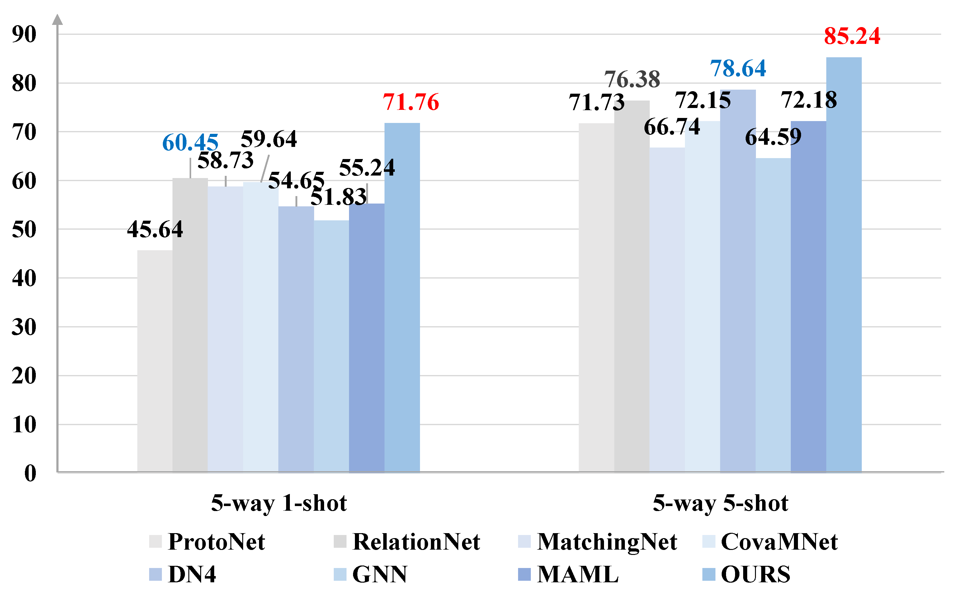
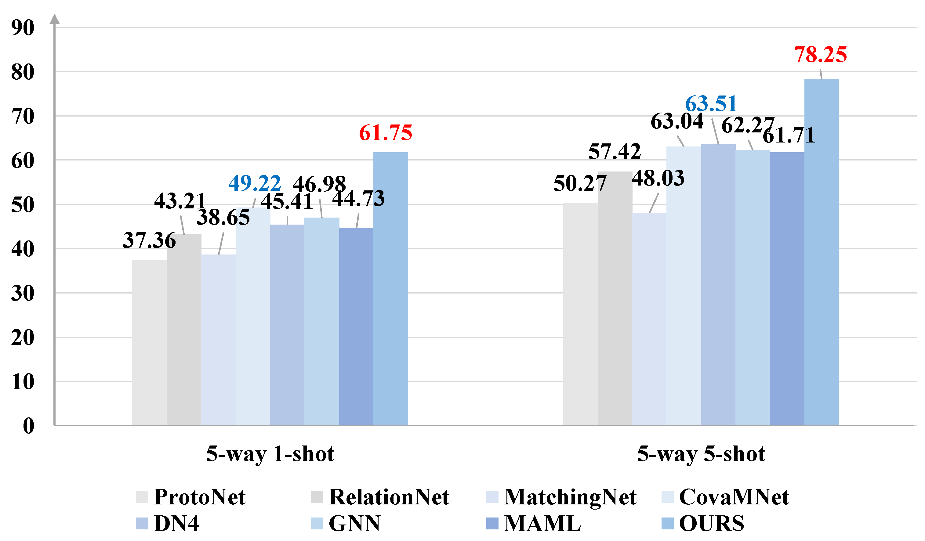
Figure 3, Figure 4 and Figure 5 summarize the results of our method on three fine-grained datasets under the 5-way–5-shot and 5-way–1-shot settings, respectively. Unlike the above-mentioned conventional datasets, Stanford Dogs, Stanford Cars, and CUB-200 are fine-grained datasets, which are even more challenging.
Here, the feature extractor we adopt is the Conv-64F backbone. Our proposed method achieves state-of-the-art performances in all three fine-grained datasets compared with the other most advanced methods, especially the Stanford Dogs dataset. Under the 5-way–5-shot setting, our method gained the largest absolute improvement over the second-best method, i.e., DN4, by 13.74%.

4.5. Experiments on Fine-Grained Few-Shot Classification Datasets

In this section, we perform extensive ablation experiments. First, we explore the effectiveness of different components in our proposed method. Then, we design some visualization cases to analyze the effectiveness of the attention mechanism dSE.

4.5.1. Effectiveness of Different Components

We performed ablation experiments on three challenging fine-grained datasets to prove the universality of the performance of each component. The experimental results are listed in Figure 6, Figure 7 and Figure 8. The baseline is the model with only channel-level feature embedding representation and cross-entropy loss. We also mark the growth rate with gray arrows.
Compared with the baseline, the model with the “channel+dSE” set performed well, as shown in Figure 6, Figure 7 and Figure 8. For the Stanford Cars dataset, the performance had a significant improvement from the baseline by 9.85% (70.36% vs. 60.51%) when employing the dSE. The accuracy of the model using pixel-level and channel-level feature representations is higher than those of the methods only using channel-level feature representation. As shown in Figure 8, the method using channel-level feature representation improved by almost 4.18% (from 64.16% to 68.34%) on the 5-way–5-shot task. Comparing the results of the last two groups of experiments in Figure 6, Figure 7 and Figure 8, we found that the accuracy improved when employing our loss function instead of the cross-entropy loss in our mode for fine-grained few-shot image classification tasks.

4.5.2. Effectiveness of Attention Mechanism dSE

To show the benefits of attention mechanism dSE in our model, we compare the grad-cam activation maps of SE and dSE, respectively, in Figure 9. These experiments were conducted on Stanford Dogs, CUB-200, and miniImageNet with the Conv-64F backbone. As Figure 9 shows, the backbone with dSE can obtain more discriminative features of the object. For example, on the Stanford Dogs dataset, the model can clearly highlight the dog’s eyes, ears, and feet (if not obscured in the image) when using dSE, which are the parts of the dogs that are easy to distinguish. For miniImageNet, the last three columns show that the model employing dSE pays more attention to the foreground objects rather than the background with noise.

5. Experimental Analysis

In this paper, we conducted extensive experiments on four common few-shot classification datasets and three challenging fine-grained benchmark datasets to validate the proposed method. We took the 5-way–1-shot and 5-way–5-shot classification tasks, and Conv-64F and ResNet-12 networks were employed as the embedding networks. Table 1, Table 2, Table 3 and Table 4 show the results of the experiments on four common few-shot classification datasets, which demonstrate that our proposed method performs better compared with other state-of-the-art methods. By employing the shallow network Conv-64F as the embedding network, we carried out experiments on the more challenging fine-grained benchmark datasets to further verify the validity and feasibility of our model. The results show that our method gains significant improvement. Notably, the accuracy for the 5-way–5-shot classification task on the Stanford Cars dataset approached 92.36% when employing our model. To verify the efficacy of different components in our method, extensive ablation experiments were performed on fine-grained few-shot classification datasets. Our method gained significant improvement in precision compared with the benchmark on Stanford Dogs due to the utilization of multi-feature embedding representation, dSE attention, and our loss function. To verify the value of the proposed dSE attention module, we show the results of the SE attention and dSE attention by the Grad-class activation maps. The backbone with dSE can extract more discriminative features of the object. Various experiments demonstrate the effectiveness of our method on few-shot image classification tasks.

6. Conclusions

In this work, we propose a novel few-shot learning method based on double pooling squeeze and excitation attention (dSE) for the purpose of improving the discriminative ability of the model by proposing a novel feature expression. Both the pixel descriptor and channel local descriptor are employed to capture locally identifiable channel features and pixel features of an image. Global max pooling and average pooling are designed to emphasize features responding to foreground object channels in the proposed dSE module. Additionally, our loss function is designed to capture the bi-directional selection relationships between query classes and support classes. A great number of comparative experiments and ablation results demonstrate that the classification performance of the method is superior to other existing approaches. In future work, we will explore more appropriate and efficient metric methods to measure query images and support set relationships.

Author Contributions

Conceptualization, Q.X.; methodology, Q.X. and J.S.; software, Q.X.; validation, Q.X.; formal analysis, Q.X. and J.S.; investigation, Q.X. and J.S.; resources, J.Z. and Y.Z.; data curation, Q.X. writing—original draft preparation, Q.X. and Y.W.; writing—review and editing, Q.X.; visualization, Q.X.; supervision, Q.X. and J.S.; Q.X. and J.S. designed the study; Q.X. analyzed and interpreted the data; Q.X. conducted the experiments, Q.X. and J.S. provided the technical and material support. All authors contributed to the writing of the manuscript and final approval. All authors have read and agreed to the published version of the manuscript.

Funding

This research was funded by the Natural Science Foundation of China under grant no. 52171310, the National Natural Science Foundation of China (no. 52001039), the Science, Technology on Underwater Vehicle Technology Laboratory (no. 2021JCJQ-SYSJJ-LB06903), Shandong Natural Science Foundation in China (no. ZR2019LZH005), and Shandong Small and Medium Enterprises Innovation Improvement Project (no. 2021TSGC1012).

Data Availability Statement

The data used to support the findings of this study are available from the corresponding author upon request.

Acknowledgments

The authors thank the anonymous reviewers for their valuable comments and suggestions.

Conflicts of Interest

The authors declare no conflict of interest.

References

  1. Wertheimer, D.; Hariharan, B. Few-shot learning with localization in realistic settings. In Proceedings of the IEEE/CVF Conference on Computer Vision and Pattern Recognition, Long Beach, CA, USA, 15–20 June 2019; pp. 6558–6567. [Google Scholar]
  2. Lifchitz, Y.; Avrithis, Y.; Picard, S.; Bursuc, A. Dense classification and implanting for few-shot learning. In Proceedings of the IEEE/CVF Conference on Computer Vision and Pattern Recognition, Long Beach, CA, USA, 15–20 June 2019; pp. 9258–9267. [Google Scholar]
  3. Xu, W.; Xu, Y.; Wang, H.; Tu, Z. Attentional constellation nets for few-shot learning. In Proceedings of the International Conference on Learning Representations, Virtual, 3–7 May 2021. [Google Scholar]
  4. Kang, D.; Kwon, H.; Min, J.; Cho, M. Relational embedding for few-shot classification. In Proceedings of the IEEE/CVF In-ternational Conference on Computer Vision, Montreal, BC, Canada, 10–17 October 2021; pp. 8822–8833. [Google Scholar]
  5. Cao, K.; Brbic, M.; Leskovec, J. Concept learners for few-shot learning. arXiv 2020, arXiv:2007.07375. [Google Scholar]
  6. Li, H.; Eigen, D.; Dodge, S.; Zeiler, M.; Wang, X. Finding task-relevant features for few-shot learning by category traversal. In Proceedings of the IEEE/CVF Conference on Computer Vision and Pattern Recognition, Long Beach, CA, USA, 15–20 June 2019; pp. 1–10. [Google Scholar]
  7. Chen, H.; Li, H.; Li, Y.; Chen, C. Multi-level metric learning for few-shot image recognition. In Proceedings of the International Conference on Artificial Neural Networks, Bristol, UK, 6–9 September 2022; Springer: Cham, Switzerland, 2022; pp. 243–254. [Google Scholar]
  8. Sell, J.; Swersky, K.; Zemel, R. Prototypical networks for few-shot learning. In Proceedings of the 31st International Conference on Neural Information Processing Systems, Long Beach, CA, USA, 4–9 December 2017; pp. 4080–4090. [Google Scholar]
  9. Vinyals, O.; Blundell, C.; Lillicrap, T.; Wierstra, D. Matching networks for one shot learning. Adv. Neural Inf. Process. Syst. 2016, 29, 3630–3638. [Google Scholar]
  10. Li, W.; Wang, L.; Xu, J.; Huo, J.; Gao, Y.; Luo, J. Revisiting local descriptor based image-to-class measure for few-shot learning. In Proceedings of the IEEE/CVF Conference on Computer Vision and Pattern Recognition, Long Beach, CA, USA, 15–20 June 2019; pp. 7260–7268. [Google Scholar]
  11. Huang, H.; Wu, Z.; Li, W.; Huo, J.; Gao, Y. Local descriptor-based multi-prototype network for few-shot learning. Pattern Recognit. 2021, 116, 107935. [Google Scholar] [CrossRef]
  12. Koch, G.; Zemel, R.; Salakhutdinov, R. Siamese neural networks for one-shot image recognition. In Proceedings of the ICML Deep Learning Workshop, Lille, France, 6–11 July 2015; Volume 2. [Google Scholar]
  13. Simon, C.; Koniusz, P.; Nock, R.; Harandi, M. Adaptive subspaces for few-shot learning. In Proceedings of the IEEE/CVF Conference on Computer Vision and Pattern Recognition, Seattle, WA, USA, 13–19 June 2020; pp. 4136–4145. [Google Scholar]
  14. Zhang, C.; Cai, Y.; Lin, G.; Shen, C. Deepemd: Differentiable earth mover’s distance for few-shot learning. IEEE Trans. Pattern Anal. Mach. Intell. 2022, 1–17. [Google Scholar] [CrossRef] [PubMed]
  15. Sung, F.; Yang, Y.; Zhang, L.; Xiang, T.; Torr, P.H.; Hospedales, T.M. Learning to compare: Relation network for few-shot learning. In Proceedings of the IEEE Conference on Computer Vision and Pattern Recognition, Salt Lake City, UT, USA, 18–23 June 2018; pp. 1199–1208. [Google Scholar]
  16. Li, W.; Xu, J.; Huo, J.; Wang, L.; Gao, Y.; Luo, J. Distribution consistency based covariance metric networks for few-shot learning. In Proceedings of the AAAI Conference on Artificial Intelligence, Honolulu, HI, USA, 27 January–1 February 2019; Volume 33, pp. 8642–8649. [Google Scholar]
  17. Zheng, Y.; Wang, R.; Yang, J.; Xue, L.; Hu, M. Principal characteristic networks for few-shot learning. J. Vis. Commun. Image Represent. 2019, 59, 563–573. [Google Scholar] [CrossRef]
  18. Finn, C.; Abbeel, P.; Levine, S. Model-agnostic meta-learning for fast adaptation of deep networks. In Proceedings of the International Conference on Machine Learning, Sydney, Australia, 6–11 August 2017; pp. 1126–1135. [Google Scholar]
  19. Mishra, N.; Rohaninejad, M.; Chen, X.; Abbeel, P. A simple neural attentive meta-learner. arXiv 2017, arXiv:1707.03141. [Google Scholar]
  20. Lee, K.; Maji, S.; Ravichandran, A.; Soatto, S. Meta-learning with differentiable convex optimization. In Proceedings of the IEEE/CVF Conference on Computer Vision and Pattern Recognition, Long Beach, CA, USA, 15–20 June 2019; pp. 10657–10665. [Google Scholar]
  21. Lu, X.; Wang, W.; Ma, C.; Shen, J.; Shao, L.; Porikli, F. See more, know more: Unsupervised video object segmentation with co-attention siamese networks. In Proceedings of the IEEE/CVF Conference on Computer Vision and Pattern Recognition, Long Beach, CA, USA, 15–20 June 2019; pp. 3623–3632. [Google Scholar]
  22. Lu, X.; Wang, W.; Shen, J.; Crandall, D.; Luo, J. Zero-shot video object segmentation with co-attention siamese networks. IEEE Trans. Pattern Anal. Mach. Intell. 2022, 44, 2228–2242. [Google Scholar] [CrossRef] [PubMed]
  23. Shen, J.; Liu, Y.; Dong, X.; Lu, X.; Khan, F.S.; Hoi, S.C. Distilled Siamese Networks for Visual Tracking. IEEE Trans. Pattern Anal. Mach. Intell. 2022, 44, 8896–8909. [Google Scholar] [CrossRef] [PubMed]
  24. Wang, X.; Girshick, R.; Gupta, A.; He, K. Non-local neural networks. In Proceedings of the IEEE Conference on Computer Vision and Pattern Recognition, Salt Lake City, UT, USA, 18–23 June 2018; pp. 7794–7803. [Google Scholar]
  25. Hu, J.; Shen, L.; Sun, G. Squeeze-and-excitation networks. In Proceedings of the IEEE Conference on Computer Vision and Pattern Recognition, Salt Lake City, UT, USA, 18–23 June 2018; pp. 7132–7141. [Google Scholar]
  26. Woo, S.; Park, J.; Lee, J.Y.; Kweon, I.S. Cbam: Convolutional block attention module. In Proceedings of the European Conference on Computer Vision (ECCV), Munich, Germany, 8–14 September 2018; pp. 3–19. [Google Scholar]
  27. Fu, J.; Liu, J.; Tian, H.; Li, Y.; Bao, Y.; Fang, Z.; Lu, H. Dual attention network for scene segmentation. In Proceedings of the IEEE/CVF Conference on Computer Vision and Pattern Recognition, Long Beach, CA, USA, 15–20 June 2019; pp. 3146–3154. [Google Scholar]
  28. Jiang, Z.; Kang, B.; Zhou, K.; Feng, J. Few-shot classification via adaptive attention. arXiv 2020, arXiv:2008.02465. [Google Scholar]
  29. Lim, J.S.; Astrid, M.; Yoon, H.J.; Lee, S.I. Small object detection using context and attention. In Proceedings of the 2021 International Conference on Artificial Intelligence in Information and Communication (ICAIIC), Jeju Island, South Korea, 13–16 April 2021; pp. 181–186. [Google Scholar]
  30. Li, T.; Li, Z.; Luo, A.; Rockwell, H.; Farimani, A.B.; Lee, T.S. Prototype memory and attention mechanisms for few shot image generation. In Proceedings of the International Conference on Learning Representations, Virtual Event, Austria, 3–7 September 2021. [Google Scholar]
  31. Yang, L.; Li, L.; Zhang, Z.; Zhou, X.; Zhou, E.; Liu, Y. Dpgn: Distribution propagation graph network for few-shot learning. In Proceedings of the IEEE/CVF Conference on Computer Vision and Pattern Recognition, Seattle, WA, USA, 13–19 June 2020; pp. 13390–13399. [Google Scholar]
  32. Oh, J.; Yoo, H.; Kim, C.; Yun, S.Y. BOIL: Towards representation change for few-shot learning. In Proceedings of the International Conference on Learning Representations, Addis Ababa, Ethiopia, 26–30 April 2020. [Google Scholar]
  33. Ye, H.J.; Hu, H.; Zhan, D.C.; Sha, F. Few-shot learning via embedding adaptation with set-to-set functions. In Proceedings of the IEEE/CVF Conference on Computer Vision and Pattern Recognition, Seattle, WA, USA, 13–19 June 2020; pp. 8808–8817. [Google Scholar]
  34. Chen, Z.; Ge, J.; Zhan, H.; Huang, S.; Wang, D. Pareto self-supervised training for few-shot learning. In Proceedings of the IEEE/CVF Conference on Computer Vision and Pattern Recognition, New Orleans, LA, USA, 18–24 June 2021; pp. 13663–13672. [Google Scholar]
  35. Wertheimer, D.; Tang, L.; Hariharan, B. Few-shot classification with feature map reconstruction networks. In Proceedings of the IEEE/CVF Conference on Computer Vision and Pattern Recognition, New Orleans, LA, USA, 18–24 June 2021; pp. 8012–8021. [Google Scholar]
  36. Zhou, Z.; Qiu, X.; Xie, J.; Wu, J.; Zhang, C. Binocular mutual learning for improving few-shot classification. In Proceedings of the IEEE/CVF International Conference on Computer Vision, Montreal, QC, Canada, 10–17 October 2021; pp. 8402–8411. [Google Scholar]
  37. Xie, J.; Long, F.; Lv, J.; Wang, Q.; Li, P. Joint Distribution Matters: Deep Brownian Distance Covariance for Few-Shot Classification. In Proceedings of the IEEE/CVF Conference on Computer Vision and Pattern Recognition, New Orleans, LA, USA, 18–24 June 2022; pp. 7972–7981. [Google Scholar]
  38. Zhang, M.; Zhang, J.; Lu, Z.; Xiang, T.; Ding, M.; Huang, S. IEPT: Instance-level and episode-level pretext tasks for few-shot learning. In Proceedings of the International Conference on Learning Representations, Addis Ababa, Ethiopia, 26–30 September 2020. [Google Scholar]
  39. Afrasiyabi, A.; Lalonde, J.F.; Gagné, C. Mixture-based feature space learning for few-shot image classification. In Proceedings of the IEEE/CVF International Conference on Computer Vision, Montreal, QC, Canada, 10–17 October 2021; pp. 9041–9051. [Google Scholar]
  40. Xu, C.; Fu, Y.; Liu, C.; Wang, C.; Li, J.; Huang, F.; Xue, X. Learning dynamic alignment via meta-filter for few-shot learning. In Proceedings of the IEEE/CVF Conference on Computer Vision and Pattern Recognition, Montreal, QC, Canada, 10–17 October 2021; pp. 5182–5191. [Google Scholar]
  41. Kim, J.; Kim, H.; Kim, G. Model-agnostic boundary-adversarial sampling for test-time generalization in few-shot learning. In Proceedings of the European Conference on Computer Vision, Glasgow, UK, 23–28 August 2020; Springer: Cham, Switzerland, 2020; pp. 599–617. [Google Scholar]
  42. Liu, Y.; Schiele, B.; Sun, Q. An ensemble of epoch-wise empirical bayes for few-shot learning. In Proceedings of the European Conference on Computer Vision, Glasgow, UK, 23–28 August 2020; Springer: Cham, Switzerland, 2020; pp. 404–421. [Google Scholar]
  43. Zhang, C.; Ding, H.; Lin, G.; Li, R.; Wang, C.; Shen, C. Meta navigator: Search for a good adaptation policy for few-shot learning. In Proceedings of the IEEE/CVF International Conference on Computer Vision, Montreal, QC, Canada, 10–17 October 2021; pp. 9435–9444. [Google Scholar]
  44. Wu, J.; Zhang, T.; Zhang, Y.; Wu, F. Task-aware part mining network for few-shot learning. In Proceedings of the IEEE/CVF International Conference on Computer Vision, Montreal, QC, Canada, 10–17 October 2021; pp. 8433–8442. [Google Scholar]
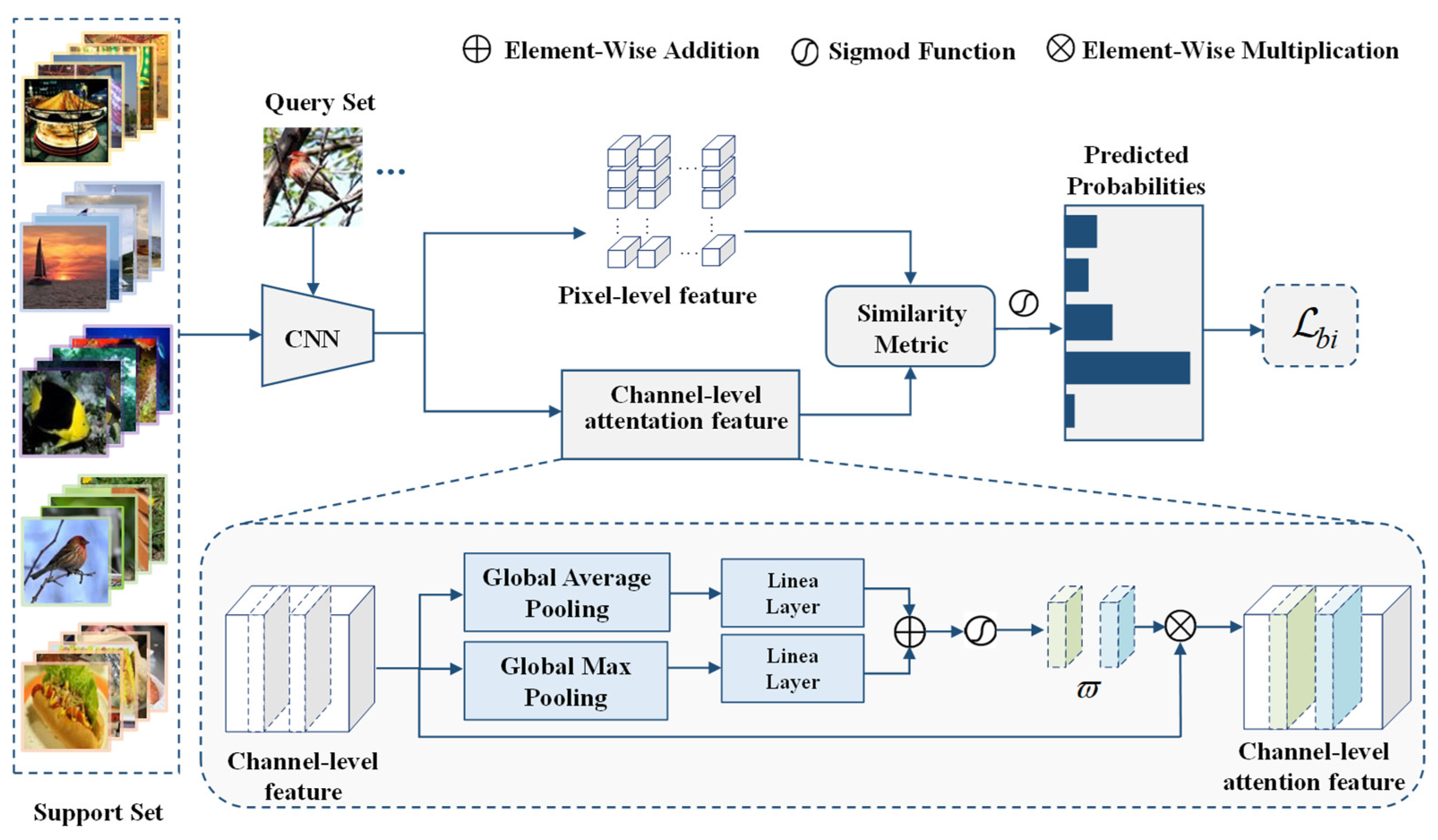
Figure 1. The framework of few-shot learning based on dSE attention. Features obtained by a backbone are expressed as pixel-level features and channel-level features, respectively. The channel-level features are fed into a double pooling squeeze and excitation (dSE) attention module to obtain the channel-level attention features, which, along with the pixel-level features, are input into a similarity metric to obtain the predicted class probability. L b i is defined to improve the robustness of the model by making the best of the bi-directional selection relationship between queries and support classes.
Electronics 12 00027 g001
Figure 2. The structure of dSE. Global average pooling and global max pooling are applied in the dSE model. Attention maps shown by grad-cam activation describe the roles of the dSE model.
Electronics 12 00027 g002
Figure 3. Classification accuracies on Stanford Cars with 95% confidence intervals. The highest and second highest results are shown in red and blue bold fonts, respectively.
Electronics 12 00027 g003
Figure 4. Classification accuracies on CUB 200 with 95% confidence intervals. The highest and second highest results are shown in red and blue bold fonts, respectively.
Electronics 12 00027 g004
Figure 5. Classification accuracies on Stanford Dogs with 95% confidence intervals. The highest and second highest results are shown in red and blue bold fonts, respectively.
Electronics 12 00027 g005
Figure 6. Effectiveness of different components. The experiments were conducted on the Stanford Cars dataset for the 5-way–1-shot/5-shot classification tasks with 95% confidence intervals. The best results are shown in bold red fonts.
Electronics 12 00027 g006
Figure 7. Effectiveness of different components. The experiments were conducted on the CUB-200 dataset for the 5-way–1-shot/5-shot classification tasks with 95% confidence intervals. The best results are shown in bold red fonts.
Electronics 12 00027 g007
Figure 8. Effectiveness of different components. The experiments were conducted on the Stanford Dogs dataset for the 5-way–1-shot/5-shot classification tasks with 95% confidence intervals. The best results are shown in bold red fonts.
Electronics 12 00027 g008
Figure 9. Grad-class activation mapping (Grad-cam) visualization results on the few-shot classification tasks. The ground-truth label is shown on the top of each input image. We compare the visualization results of the dSE-integrated network (Conv-64F + dSE) and SE-integrated network (Conv-64F + SE) in the next two rows.
Electronics 12 00027 g009
Table 1. Comparison of the state-of-the-art methods with 95% confidence intervals on miniImageNet. The highest and second highest results are shown in red and blue bold font for easy observation and analysis.
MethodBackbone5-way–1-shot5-way–5-shot
BOIL [32]Conv-64F49.61 ± 0.1666.45 ± 0.37
ProtoNet [8]Conv-64F49.42 ± 0.7868.20 ± 0.66
CovaMNet [16]Conv-64F51.19 ± 0.7667.65 ± 0.63
DN4 [10]Conv-64F51.24 ± 0.7471.02 ± 0.64
DSN [13]Conv-64F51.78 ± 0.9668.99 ± 0.69
FEAT [33]Conv-64F55.15 ± 0.2071.61 ± 0.16
OURSConv-64F59.42 ± 0.5177.36 ± 0.73
PSST [34]ResNet-1264.05 ± 0.4980.24 ± 0.45
ConstellationNet [5]ResNet-1264.89 ± 0.2379.95 ± 0.37
FRN [35]ResNet-1266.45 ± 0.1982.83 ± 0.13
DeepEMD [14]ResNet-1265.91 ± 0.8279.74 ± 0.56
BML [36]ResNet-1267.04 ± 0.6383.63 ± 0.29
Meta DeepBDC [37]ResNet-1267.34 ± 0.4384.46 ± 0.28
OURSResNet-1269.64 ± 0.4487.95 ± 0.53
Table 2. Comparison of the state-of-the-art methods with 95% confidence intervals on tieredImageNet. The highest and second highest results are shown in red and blue bold font for easy observation and analysis.
MethodBackbone5-way–1-shot5-way–5-shot
ProtoNet [8]Conv-64F48.67 ± 0.8769.57 ± 0.75
BOIL [32]Conv-64F49.35 ± 0.2669.37 ± 0.12
DN4 [10]Conv-64F53.37 ± 0.8674.45 ± 0.70
CovaMNet [16]Conv-64F54.98 ± 0.9071.51 ± 0.75
IEPT [38]Conv-64F58.25 ± 0.4875.63 ± 0.46
OURSConv-64F61.47 ± 0.8379.56 ± 0.64
RelationNet [15]ResNet-1258.99 ± 0.8675.78 ± 0.76
DSN [13]ResNet-1267.39 ± 0.8282.85 ± 0.56
MixtFSL [39]ResNet-1270.97 ± 1.0386.16 ± 0.67
FEAT [33]ResNet-1270.80 ± 0.2384.79 ± 0.16
DeepEMD [14]ResNet-1271.16 ± 0.8783.95 ± 0.58
RENet [4]ResNet-1271.61 ± 0.5185.28 ± 0.35
DMF [40]ResNet-1271.89 ± 0.5285.96 ± 0.35
OURSResNet-1275.25 ± 0.6489.21 ± 0.46
Table 3. Comparison of state-of-the-art methods with 95% confidence intervals on CIFAR-FS. The highest and second highest results are shown in red and blue bold font for easy observation and analysis.
MethodBackbone5-way–1-shot5-way–5-shot
ProtoNet [8]Conv-64F55.50 ± 0.7072.00 ± 0.60
ConstellationNet [5]Conv-64F69.30 ± 0.3082.70 ± 0.20
OURSConv-64F69.70 ± 0.4287.56 ± 0.44
MetaOpt
Net [20]
ResNet-1272.00 ± 0.7084.20 ± 0.50
MABAS [41]ResNet-1273.51 ± 0.9285.49 ± 0.68
RENet [4]ResNet-1274.51 ± 0.4686.60 ± 0.32
OURSResNet-1277.12 ± 0.4092.85 ± 0.30
Table 4. Comparison of state-of-the-art methods with 95% confidence intervals on FC100. The highest and second highest results are shown in red and blue bold font for easy observation and analysis.
MethodBackbone5-way–1-shot5-way–5-shot
MetaOptNet [20]ResNet-1241.10 ± 0.6055.50 ± 0.60
ProtoNet [8]ResNet-1241.54 ± 0.7657.08 ± 0.76
E3BM [42]ResNet-1243.20 ± 0.3060.20 ± 0.30
ConstellationNet [5]ResNet-1243.80 ± 0.2059.70 ± 0.20
MixtFSL [39]ResNet-1244.89 ± 0.6360.70 ± 0.60
Meta Navigator [43]ResNet-1246.40 ± 0.8161.33 ± 0.71
DeepEMD [14]ResNet-1246.47 ± 0.7863.22 ± 0.71
TPMN [44]ResNet-1246.93 ± 0.7163.26 ± 0.74
OURSResNet-1250.32 ± 0.7371.55 ± 0.75
Disclaimer/Publisher’s Note: The statements, opinions and data contained in all publications are solely those of the individual author(s) and contributor(s) and not of MDPI and/or the editor(s). MDPI and/or the editor(s) disclaim responsibility for any injury to people or property resulting from any ideas, methods, instructions or products referred to in the content.