This section uses CenterNet as the basic model to explore the influence of the size, depth, and fusion mechanism of the backbone network’s convolution features on multi-scale target ships and find the best convolution feature settings in each scale range.
3.1. The Structure and Principle of the CenterNet Model
We chose CenterNet [
14] as the basic pdetection framework and Resnet50 [
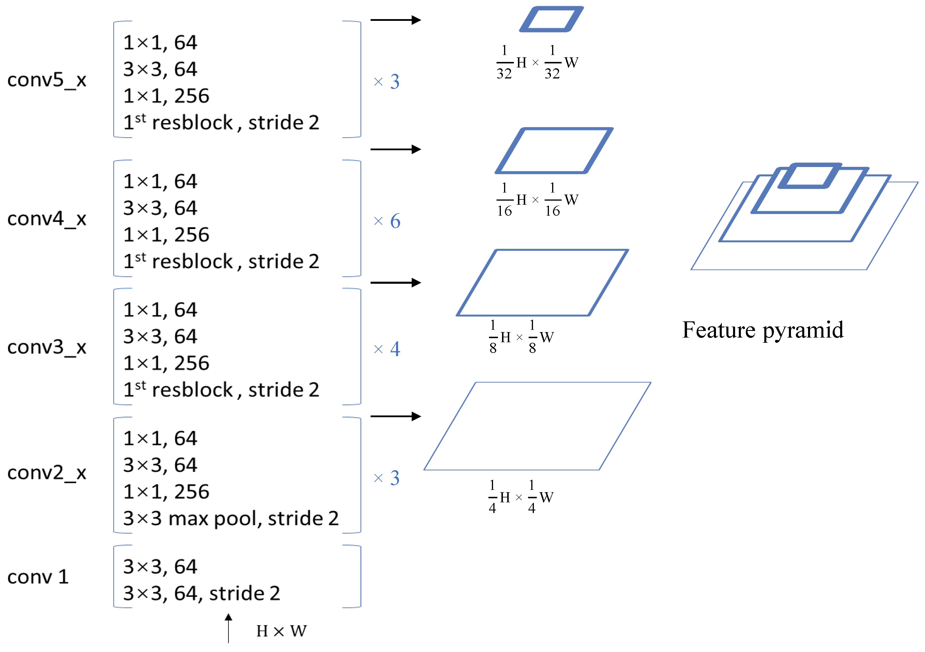
28] as the basic backbone network for feature extraction. The backbone network structure is shown in
Figure 1, consisting of a total of 5 network segments:
,
,
,
, and
.
The original first network segment
is a single-layer convolutional network with a core of
and a step size of 2. We used two convolutional layers with a core of
instead, where the first convolutional layer has a step size of 2. The second network segment is composed of three identical residual blocks in series, and there is a maximum pooling layer with a core of
and a step length of 2 before the residual block. The third network segment is composed of 4 identical residual blocks in series. In the first residual block of the network segment, the convolutional layer with a core of
has a step size of 2. The fourth network segment is composed of 6 identical residual blocks. In the first residual block of the network segment, the convolutional layer with a core of
has a step size of 2. The fifth network segment is composed of 3 identical residual blocks, and the step size of the convolutional layer with a core of
; the first residual block of the network segment is set to 2. It can be observed from the image input network that each time it passes through a network segment, the resolution of the output convolution feature map drops to
of the previous network segment. We use the second, third, fourth, and fifth network segment output convolution feature maps to explore the network feature fusion strategy, denoted as C2, C3, C4, and C5, respectively. Inspired by the idea of CornerNet [
15,
27] discarding anchor boxes and using corner points to represent box positions, Zhou et al. designed CenterNet. Unlike CornerNet, CenterNet uses the center point of the target box to indicate the position of the box, and the shape of the box is directly represented by its width and height. Similar to CornerNet, CenterNet does not directly predict the coordinates of the center point of the box, but it predicts the distribution of the center point of the box. The center point distribution is represented by a heat map.
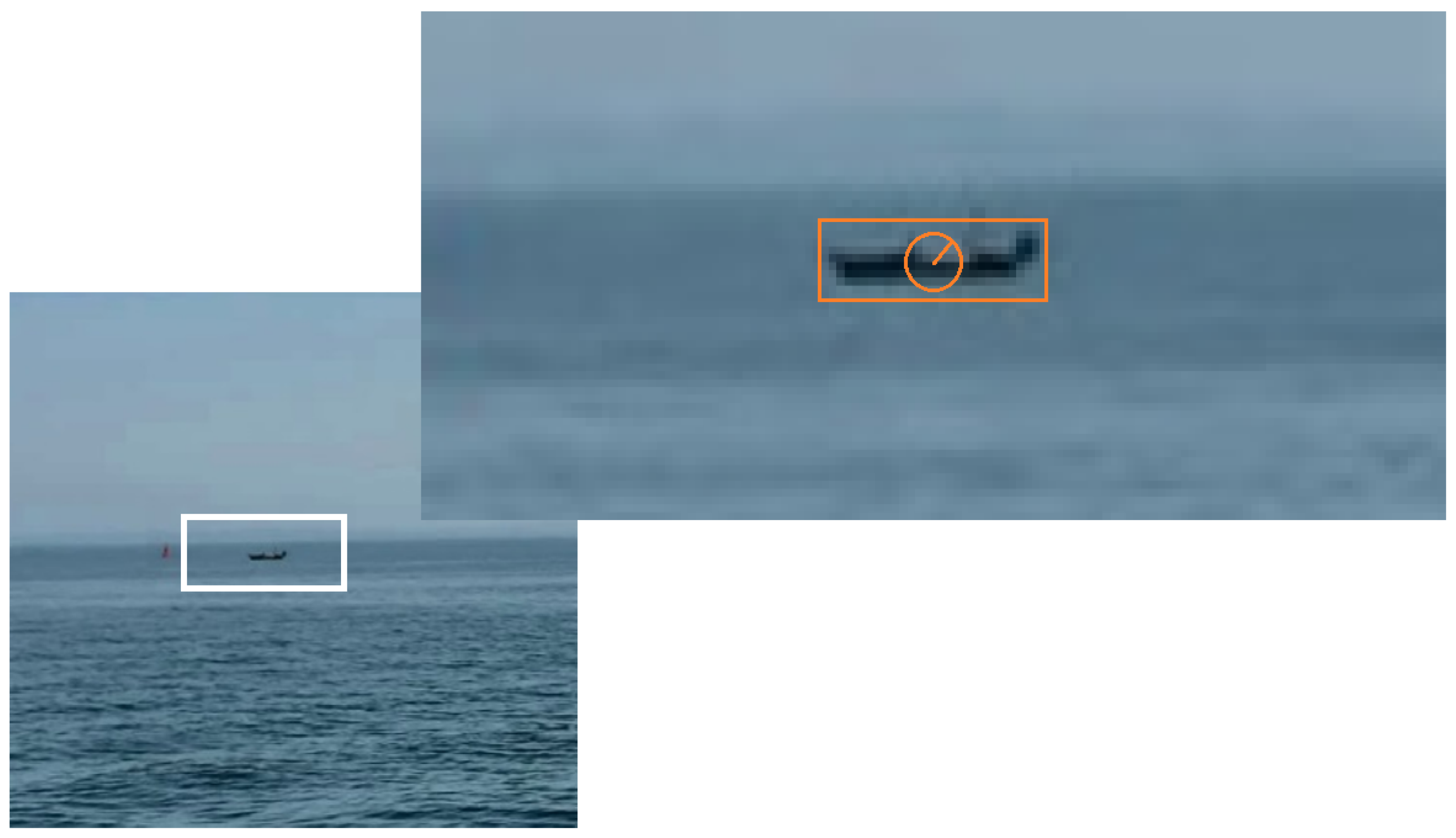
In
Figure 2, the solid red rectangular box represents the actual box marked by the ship. When the center of the yellow rectangular box is near the center of the red rectangular box, the yellow dashed box can also correctly represent the ship. This is because the red solid line frame and the yellow dashed line frame have a larger intersection ratio at this time. The closer the center of the yellow box is to the center of the red box, the greater the intersection ratio between the two; on the contrary, the smaller the intersection ratio between the two. The green circle indicates the allowable range of the center point of the yellow dashed box. When it exceeds this range, it can no longer indicate the position of the ship. We call the green circle the distribution circle, and the radius of the green circle is the distribution radius. When the width and height of the red actual label box are determined, the distribution radius
r is determined by the intersection ratio of the red and yellow boxes.
In the exploration experiment, we set , that is, the intersection ratio of the yellow box and the red box must be at least 0.7 to be marked as a positive sample. This processing can expand the number of positive sample points and reduce the impact of the imbalance of positive and negative samples when training the network. In addition, this central point representation mechanism can also improve the robustness of the model during reasoning and avoid false negative detection errors.
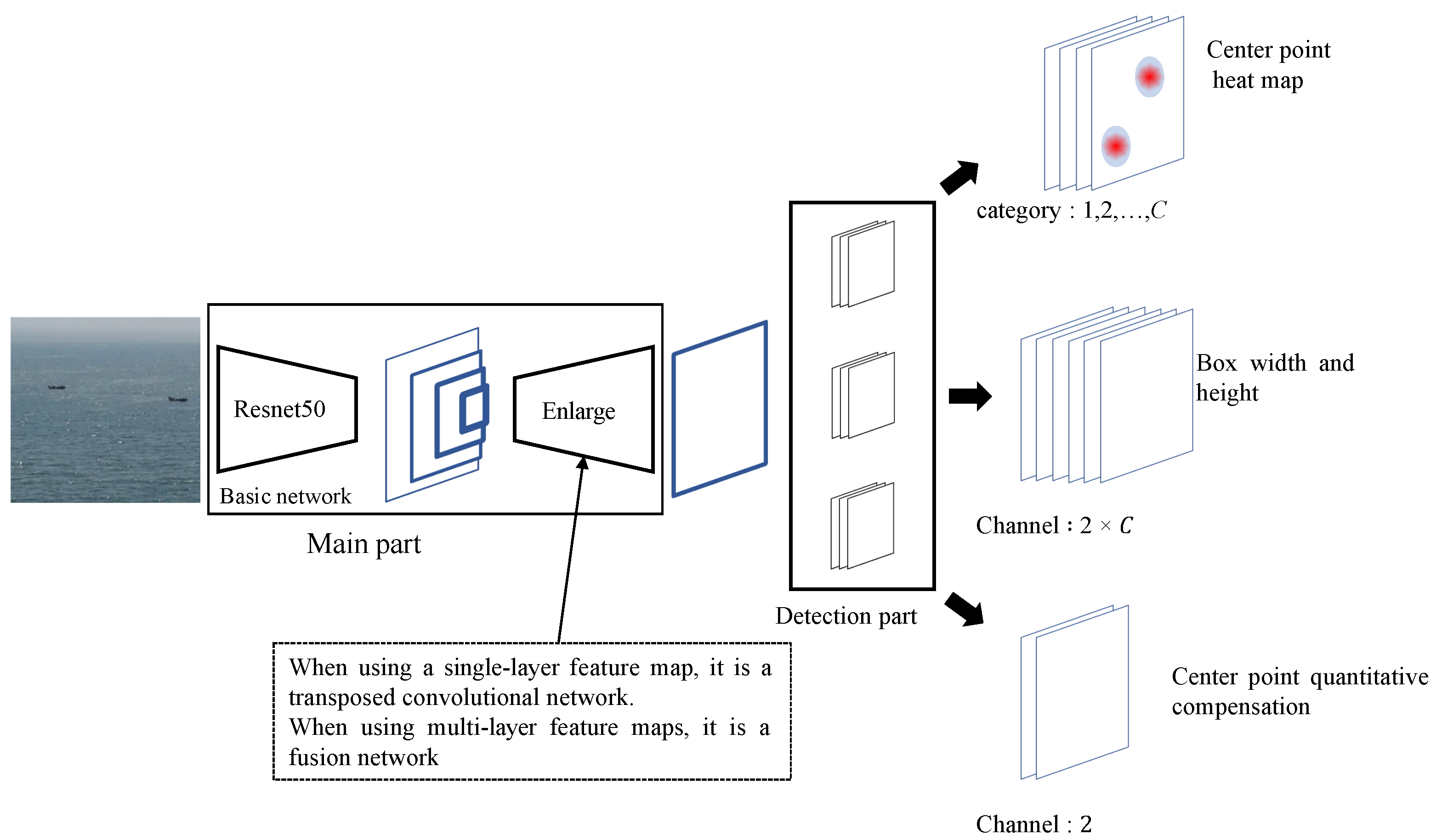
We replaced the hourglass backbone network of CenterNet with Resnet50 in the actual setting of the exploration, and used it to study the 4-layer convolution feature map of the second, third, fourth, and fifth network segments, as shown in
Figure 3. When using single-layer convolution feature map detection, the selected feature map is input into multiple consecutive transposed convolution layers, and the convolution feature map is enlarged to the required resolution; when using multi-layer convolution feature map detection, the selected feature map is input into the fusion network, and the convolution feature with the required resolution is obtained for detection. The feature map is obtained and then input to the three branches detection part. Each branch is a two-layer convolutional network. The convolution kernel of each layer is
, the step size is 1, and the number of convolution kernels in the first layer is 256; the number of second-layer convolution kernels is different. The first branch is used to predict the heat map of the center point, the second branch is used to predict the width and height of the box, and the third branch is used to predict the quantized compensation value of the center point. The output of the three branches is three tensors. The resolution of the three tensors is the same, which is determined by the feature map of the input detection network, but their numbers of channels are different. The number of channels for predicting the branch output tensor of the center point heat map is the number of sample categories. In this experiment, there is only one type of ship, so the number of channels is 1. The number of channels for predicting the branch output tensor of the box width and height is sample 2 times the number of categories; each category predicts the width and height of the sample box in its respective category. The number of channels for predicting the branch output tensor of the quantized compensation value of the center point is 2, that is, the offset value in the x and y directions.
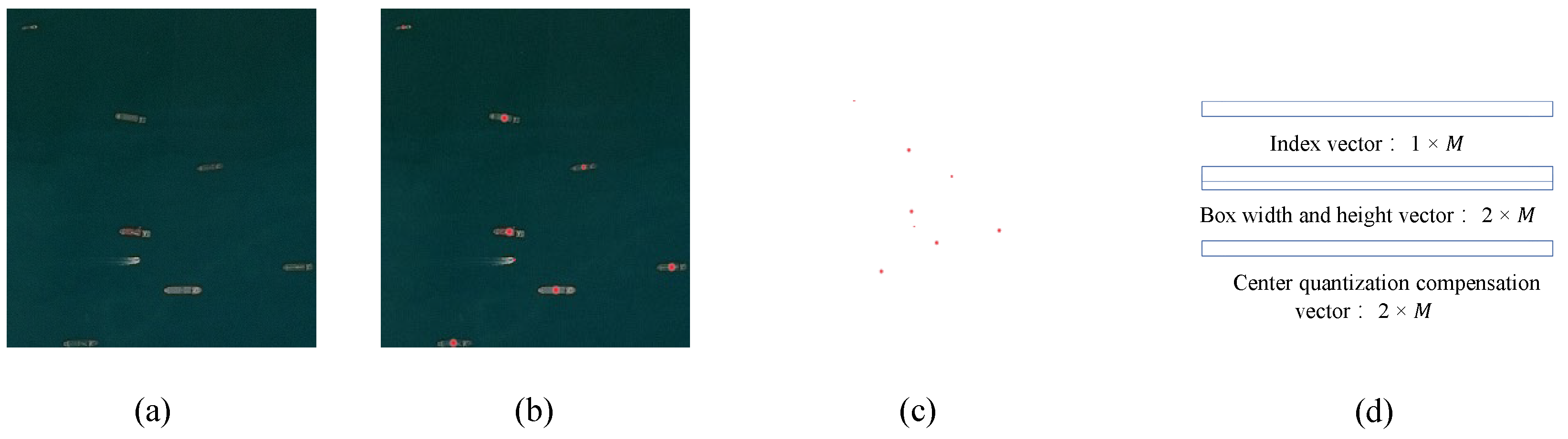
During training, the sample data used by CenterNet were converted into the form shown in
Figure 4.
Figure 4a is a training image. Taking the box of this ship as the center, a two-dimensional Gaussian distribution was generated to cover the location of the target, as shown in
Figure 4b, and the center point heat map corresponding to this image was obtained. The function that produces this two-dimensional Gaussian distribution is formulated by Equation (
1):
where
represents the coordinates of the center point of the target box, and
is
of the radius of the circle shown in
Figure 2, where the radius is determined by the width and height of the target box. In the original CenterNet network, the resolution of the center point heat map is downsampled by
from the original input, as shown in
Figure 4c. The width and height of the box and the center quantization compensation are represented by two vectors with length
M and the number of channels 2. In addition, the index vector is required to establish a mapping relationship between the center point heat map and the box width and height vector and the center quantization compensation vector, as shown in
Figure 4d.
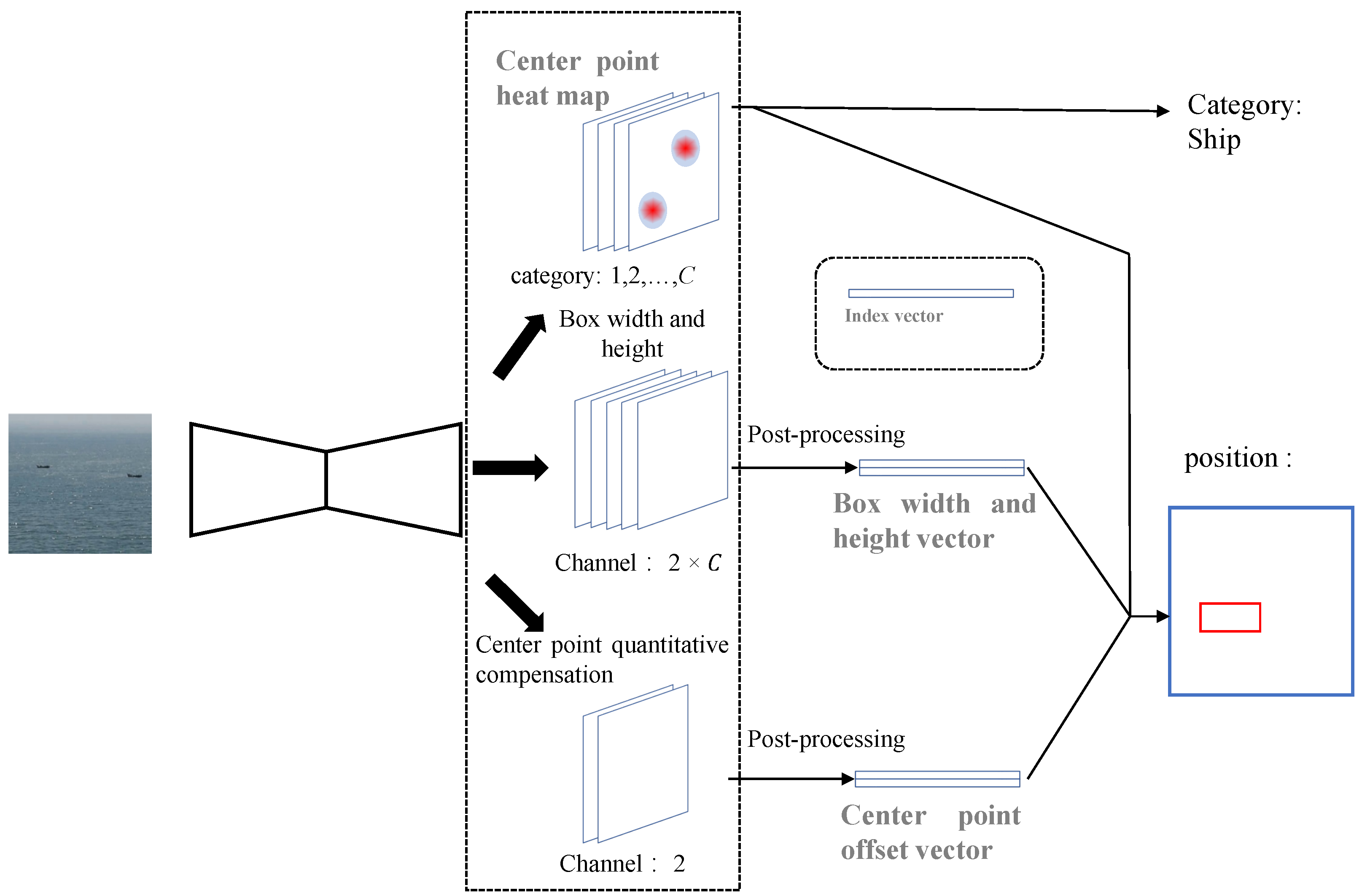
In inference, after the image was input to CenterNet, the center point heat map tensor, the center point quantization compensation value tensor, and the box width and height value tensor were obtained, as shown in
Figure 5. From the center point heat map, the center point coordinates of the box and the box category can be directly extracted. Each specific value in the box width and height value tensor and the center point quantization compensation tensor has no practical meaning but can be converted into a box width and height vector and a center point offset vector through post-processing. Combined with the extracted coordinates of the center point of the box, the final coordinate value of the box can be obtained.
3.2. The Influence of the Size of Convolution Features on Multi-Scale Ship Target Detection
We used a downsampling rate of the convolution feature relative to the input image as the size of the convolution features. For example, the size of C4 is , the size of C5 is , the size of the input image is 1, and the size of the input image obtained by upsampling 2 times is 2. The original CenterNet connects 4 layers of deconvolution layers with a step length of 2 behind C5, and the resulting convolution featurep size is .
In order to explore the influence of the convolution features of the backbonep network on the change of ship target scale, we especially studied the convolution features of C5. We connected a number of deconvolution layers with a step size of 2 and a convolution kernel after C5 so that the size could be enlarged to , , , 1 and 2.
The evaluation method is shown in
Section 4.1.2. The experimental results are shown in
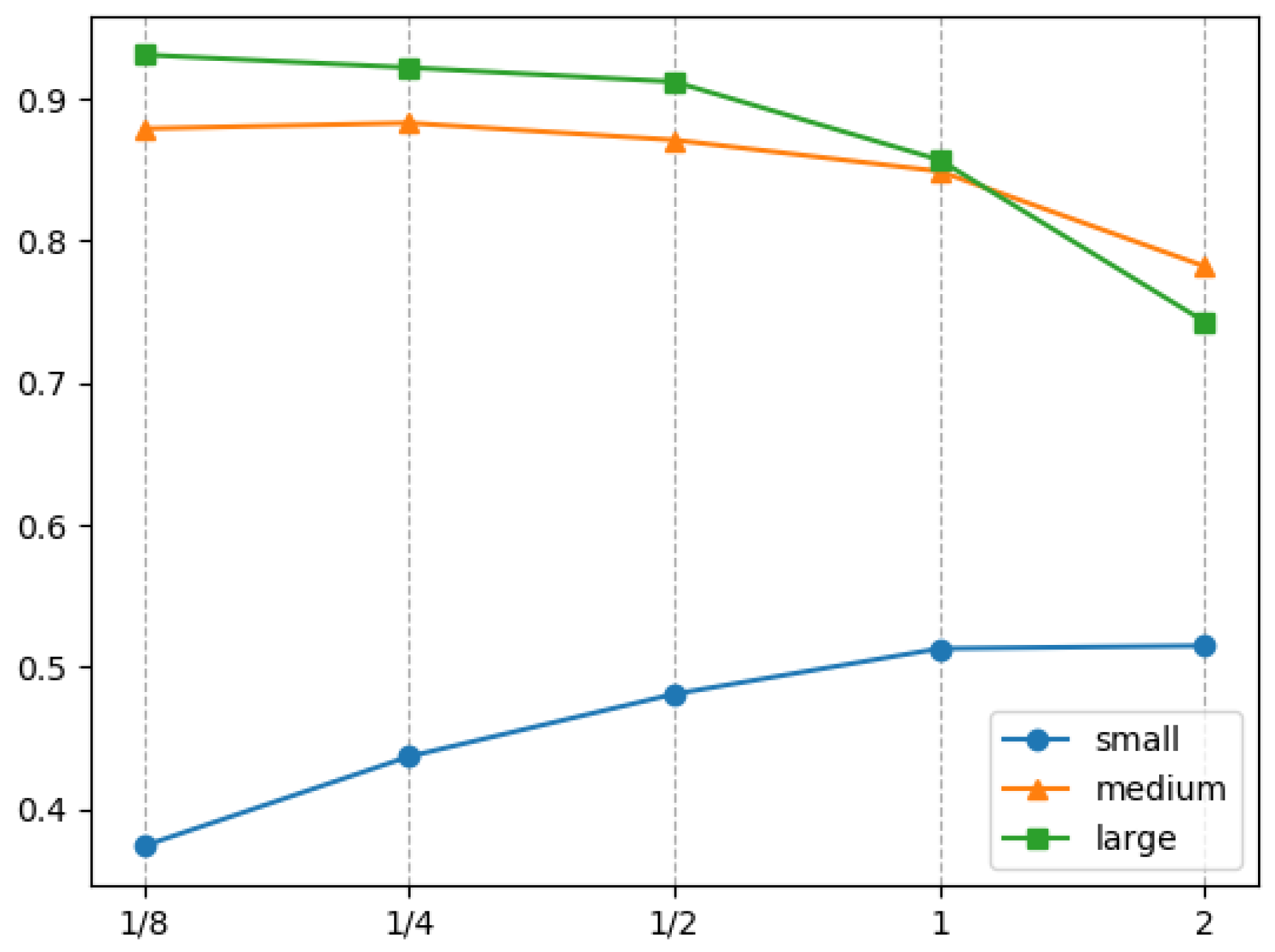
Table 1. For small-scale ship targets, the larger the size of the convolution feature output by the backbone network, the better the detection performance. For medium-scale and large-scale ship targets, better detection results were obtained using smaller-size convolution features during detection. However, as the size of the convolution feature used for detection changes, the detection accuracy gain effects of ship targets of different scales also become different, as shown in
Figure 6.
For small target ships, as the size of the convolution feature increases, the gain in detection performance obtained gradually decreases. When the size of the convolution feature increases from
to
, the detection accuracy of small target ships can be improved by
. When the convolution feature size increases from
to
and from
to 1, the detection accuracy of small target ships increases by
and
, respectively; however, when the convolution feature size is increased from 1 to 2, the detection accuracy gain of the small target ship is very slight, only
. The detection of small target ships requires a larger feature size, because this can make the receptive field smaller, and the detector does not mix too much background information when detecting small target ships; however, when the size of the convolution feature exceeds the size of the input image, it does not bring significant gain. We believe this is because the convolutional features that exceed the input size without being enhanced [
29] will not obtain more refined details. Therefore, we believe that the convolutional features with the same size as the input image are most suitable for detecting small-scale ship targets. They can obtain almost the same detection accuracy as 2 times the input size, and at the same time, the computational cost is lower.
For ships of medium target size, the best detection result is obtained when the convolution feature size is . When the convolution feature size is less than , the larger the size, the lower the detection accuracy. When the convolution feature size is greater than , the detection accuracy of the medium-sized target ship begins to decrease. When the convolution feature size decreases from to , the detection accuracy drops by . With the gradual decrease in the size of the convolution feature comes a greater decrease in the target detection accuracy of medium-sized ships, or, in other words, the greater the negative gain. When the size of the convolution feature is increased from to , the detection accuracy of medium-sized target ships is reduced by ; when the size of the convolution feature is increased from to 1, the detection accuracy is reduced by ; when the convolution feature size is increased from 1 to 2, the detection accuracy is reduced by . We believe that the most suitable convolution feature size for detecting medium-scale ship targets is of the input image. When the convolution feature size is greater than , because the receptive field is too small, the detector cannot perceive all the information of the medium-sized ship target, which reduces the detection result; when the convolution feature size is greater than , the receptive field is too large, so that the detector experiences interference from background information, which weakens the performance of the detector.
For large-scale ship targets, as the size of the convolution feature decreases, the detection performance gain obtained gradually decreases. When the size of the convolution feature is reduced from 2 to 1, the detection accuracy of large-scale ship targets can be increased by ; when the size of the convolution feature is reduced from 1 to , the detection accuracy of large-target ships is increased by . When the convolution feature size is reduced from to and from to , the detection accuracy is increased by and , respectively, and the increase is very small. Detecting large ship targets requires a larger receptive field. Using a smaller size convolution feature can enable the detector to obtain a larger receptive field and obtain better detection results. When the convolution feature size is large, the target detector receives interference from the background signal. However, compared with small and medium-sized ship targets, the detection of large-scale ship targets is less sensitive to background signals. With certain background information mixed in, the detector can also detect large-scale ship targets. Therefore, when detecting large ship targets, and when the size of the convolution feature is reduced from to , we speculate that if the detection accuracy increases, the increase will not exceed ; if the detection accuracy decreases, the drop will not be too great. According to the experimental results and analysis, we believe that the size of the input image after downsampling by is most conducive to detecting large-scale ship targets.
In addition, from
Figure 6, it can be found that the detection performance characteristics of medium-scale and large-scale ship targets regarding convolution feature size are similar in trend. However, compared with medium-scale and large-scale ship targets, the detection performance characteristics of small target ships regarding convolution feature size is significantly different. First, the detection accuracy of the convolution feature size of large-scale and medium-scale ship targets is about 75–95%, while the range of small targets is about 35–55%; second, the detection accuracy of large-scale and medium-scale ship targets tends to decrease with the increase in the convolution feature’s size, while the detection accuracy of small target ships increases with the increase of the convolution feature’s size. These two differences show that the size of the convolution feature has inconsistencies in the detection of small target ships and non-small target ships, but this inconsistency is not the main factor that leads to the poor detection accuracy of small target ships.
3.3. The Influence of the Depth of Convolution Features on Multi-Scale Ship Target Detection
C2, C3, C4, and C5 come from the output of different depth layers of Resnet50, where C2 is the output of the 11th layer, C3 is the output of the 23rd layer, C4 is the output of the 41st layer, and C5 is the output of the 50th layer. Therefore, we directly use these four convolution features to explore the influence of the depth of the backbone network convolution feature on the changes in ship target scale.
In the experiment, we first used the complete Resnet50 as the basic feature extraction network and added a 4-layer transposed convolution to enlarge the feature size. We used the trained convergent model to characterize the performance of C5; we took the C4 part of the convergent network and added 3 transposed convolutional layers, froze the weight of the C4 part during training, and only updated the network weights of the amplified part and the detected part. The resulting model was used to characterize the performance of C4. We took the C3 part of the convergence network and added 2 transposed convolutional layers, froze the weight of the C3 part during training, and only updated the weight parameters of the amplification part and the detection part, and the resulting model is used for characterization of C3’s performance. We took the C2 part of the convergence network and added a transposed convolutional layer, froze the weight of the C2 part during training, and only updated the weight parameters of the amplification part and the detection part; the resulting model was used to characterize the performance of C2. Adopting the above-mentioned experimental settings, on the one hand, prevents the interference of the convolution feature’s size; on the other hand, the weight of the shared feature extraction network remains consistent, which means that the inconsistency of the initialization parameters and the inconsistency of the convergence path are eliminated.
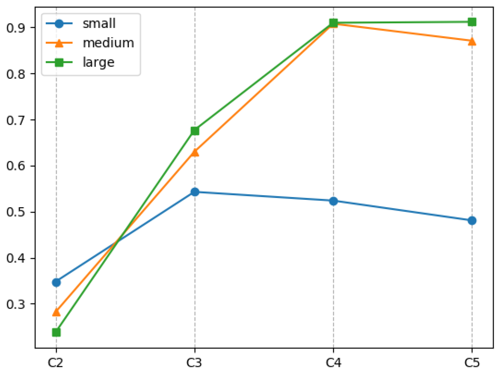
The experimental results are shown in
Table 2. Small-scale ship targets use C3 depth convolution features to obtain the best detection results; medium-scale ship targets use C4 depth convolution features to make the detection accuracy the highest; large-scale ship targets use C5 depth convolution features to make the detection accuracy the highest. Because the weight parameters of the feature extraction basic network are shared in the experiment, from the point of view of parameter fitting, for small target ships, the C3 convolution feature is just fitting, the C2 feature is under-fitting, and C4 and C4 are under-fitting. The convolutional features of the C5 layer are in an over-fitting state. For medium-sized ship targets, the C4 feature is in a fitting state, the C2 and C3 features are in an under-fitting state, and the C5 feature has entered an over-fitting state. For large-scale ships C2 and C3 are obviously under-fitting, while C4 to C5 are only increased by
, and the two are almost the same. It can be considered that C4 and C5 have reached the fitting state.
The characteristics of ship targets of different scales with respect to the depth of convolution features are shown in
Figure 7. It can be found that large- and medium-scale ship targets have strong similarities in trends, while small targets have great differences compared with them. The detection accuracy of large and medium target ships on the convolution features of C2 depth is less than
, while the detection accuracy of small target ships on the convolution features of C2 depth is
, which is higher than that of large and medium targets. The detection accuracy of large and medium targets increases rapidly when the convolution feature depth increases from C2 to C4, and it rises or decreases slightly from C4 to C5, while the detection accuracy of small targets only rises from C2 to C3 and reaches C3. After the high point, C4 and C5 slowly fall back. Through analysis, it can be seen that the detection of large- and medium-sized ship targets is more dependent on deeper convolutional layer features, while the detection of small target ship targets is more dependent on shallower convolutional layer features. In other words, the depth of the convolution feature has inconsistency in the detection of small target ships and non-small target ships. This inconsistency will aggravate the phenomenon in which the detection accuracy of small target ships is much lower than that of non-small target ships. It can be said that, among the factors that make it more difficult to detect small targets than non-small target ships, the inconsistency of the convolution feature depth on the target scale is more important than the inconsistency of the convolution feature size on the target scale.
From
Figure 6 and
Figure 7, it can be observed that whether it is about the size or depth of the convolution features, the characteristics of large and medium-sized ship targets have a strong similarity, while their characteristics and the characteristics of small target ships are very inconsistent. We believe that this similarity and inconsistency are determined by the way the convolutional network expresses the characteristics of ships of different scales.
Some studies have pointed out that the convolutional network mainly recognizes objects by extracting texture features instead of shape or color features [
30]. Texture can be characterized by spectral characteristics, and the forward process of convolutional neural networks is a multi-layer nonlinear activated filter. Many studies [
12,
31] believe that in the target detection model based on convolutional neural networks, shallow features have more accurate detailed information, while deep features have richer semantic information. The shallow layer of the convolutional network extracts fine-grained texture features with a smaller receptive field, and the deep layer extracts coarse-grained texture features with a larger receptive field. The shallow convolution features are more detailed, and as the network deepens, the expression of the convolution features becomes more and more abstract. However, the texture information of the small target itself is sparse, and the convolutional neural network can only rely on the texture feature pattern extracted in the shallow layer for detection. Large- and medium-scale targets are rich in texture information, and convolutional neural networks can only obtain their proper feature expression at a deeper level. In the deep convolutional features, the feature expression of small targets will be too abstract. Therefore, the detection results of small target ships using shallower convolution features are better than using deep convolution features, and large and medium-scale ships have to use deep convolution feature roots to obtain the best detection results. We believe that large and medium-scale ship targets have similarities in the expression of convolution features, while small target ships and non-small target ships have inconsistencies in the expression of convolution features. These similarities and inconsistencies are caused by the inherent working mode of convolutional neural networks, which can be regarded as the inherent characteristics of ship targets of different scales.
3.4. The Effect of Convolutional Feature Fusion Mechanism on Multi-Scale Ship Target Detection
There are two types of convolution feature map fusion operations: (1) adding elements element by element; (2) splicing along the channel. They can be divided into early fusion and late fusion according to the order of fusion and prediction. Early fusion refers to the fusion of multi-layer features into single-layer features, and predictions are made on the single-layer features after the fusion, such as in [
32,
33]. Late fusion refers to the use of multiple different levels of convolutional feature maps for prediction and the fusion of the detection results of multiple features. Late fusion can be divided into two categories: the first category directly uses the multi-layer features extracted by the basic network to predict, and the multi-layer prediction results are merged to obtain the final result, such as SSD [
12]; After the feature map is fused, the multi-layer fusion feature of the pyramid structure is obtained, and the prediction result of the multi-layer fusion feature is further fused to obtain the final result. FPN and PAN are the most typical representatives.
We noticed that the feature pyramid fusion adopts a layer-by-layer transfer and gradual fusion method. There are the same number of feature layers before and after the fusion, and the feature maps of the corresponding levels have the same resolution. In [
31,
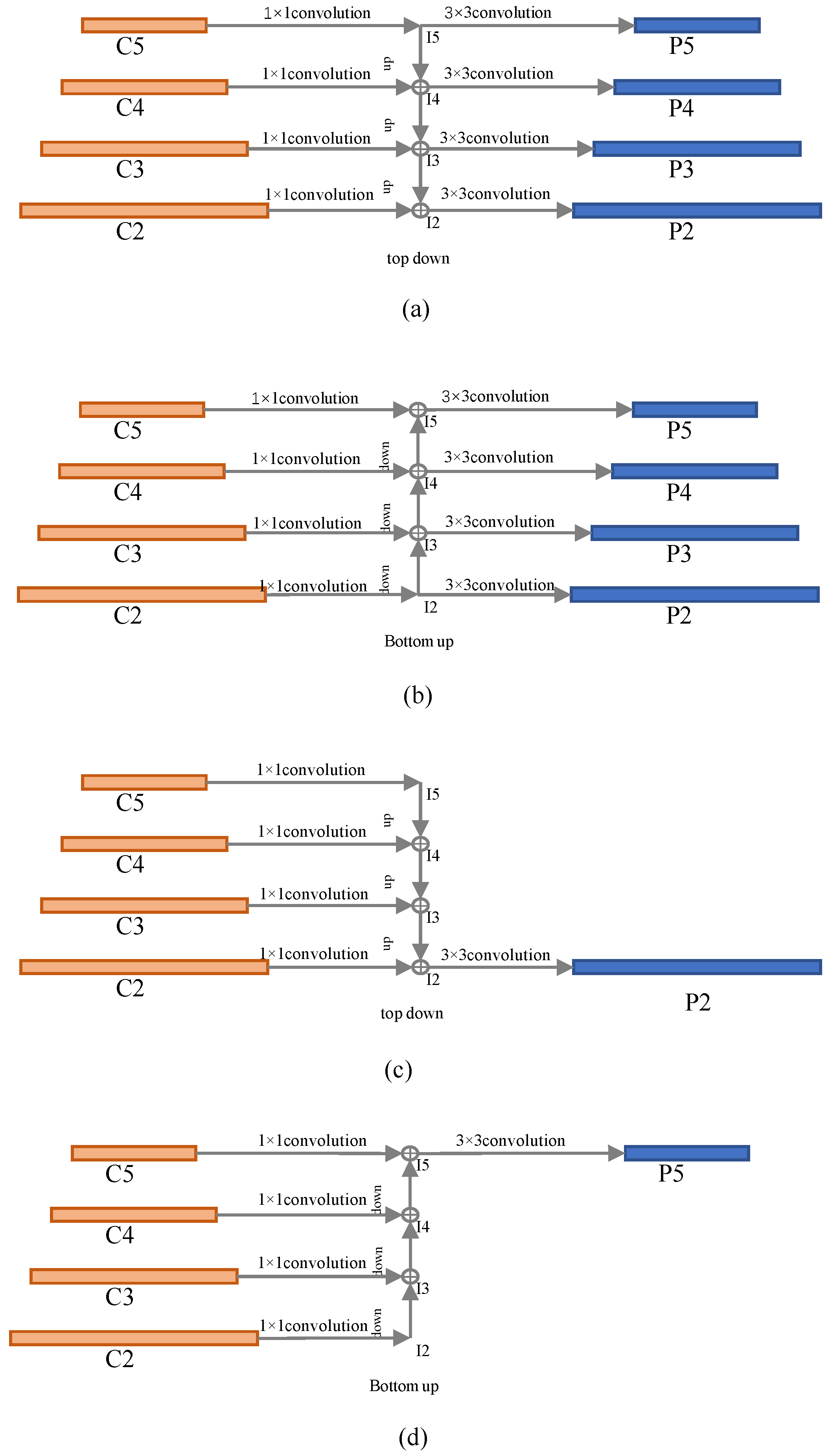
34], the feature pyramid has two fusion paths: (1) top-down and (2) bottom-up.
Figure 8a shows the top-down pyramid fusion method. The left side is the feature pyramid composed of 4 layers of tensors extracted by the basic network, which are
, and on the right is the merged feature pyramid, which are
. Before the fusion operation, a
convolution will be used to convert the feature tensor of the 4-layer basic network into the same number of channels,
N, generally set as
. The top-down fusion method starts from C5; C5 obtains I5 after
convolution, and I5 directly enters a
convolution layer to obtain P5. The up-sampling of I5 and the result of
convolution with C4 are added element-by-element to obtain I4, and I4 is obtained after a
convolution layer to obtain P4. Up-sampling I4 to double its size, adding the result to the tensor of C3 after
convolution element-by-element to obtain I3. I3 goes through a
convolution layer to obtain P3. We then upsample I3 to enlarge the size, add the result to the tensor after
convolution of C2 element by element to obtain I2, and let I2 pass through a
convolution layer to obtain P2. By observing the pyramid fusion operation process of the top-down path, it can be found that the fusion features of each layer are unequal. P5 does not incorporate the convolutional features of other layers; it is the result of C5 passing through a 2-layer convolutional network. P4 only incorporates two convolutional features of C4 and C5. C4 and C5 are finally passed to P4 through I4, but C5 is passed to I4 after I5 and upsampling. I5 will lose a certain amount of information during upsampling. C4 is directly passed to I4 through a layer of convolution with a step size of 1, so the information of C4 obtained in the fusion feature P4 is stronger than that of C5. P3 combines the three-layer convolution features of C3, C4 and C5. C4 and C5 are passed to I3 after I4 and up-sampling. At the same time, I3 integrates the characteristic information from C3. Since I4 is up-sampled and C4 is not scaled, the information of C3 obtained in the fusion feature P3 is stronger than C4, and C4 is stronger than C5. Only P2 incorporates the convolutional features of all four layers of C2, C3, C4 and C5. I3, which combines the features of C3, C4, and C5, is up-sampled and transferred to I2. At the same time, I2 combines the information passed by C2. Similar to the previous one, the information of C2 obtained in the fusion feature P2 is stronger than that of C3, and C3 is stronger than C4, while C5 has the weakest information.
Figure 8b shows the bottom-up pyramid fusion method. The difference is that the bottom-up fusion method starts from C2 and gradually transfers to each layer above. Similar to the top-down fusion path, the fusion characteristics of each layer of the bottom-up fusion path are not equal. The difference is that in the bottom-up feature pyramid, P2 does not integrate the feature information of any other layers. It is only obtained by C2 through a two-layer convolutional network. P3 combines the two-layer convolution features of C3 and C2. C2 is fused with C3 through I2 downsampling to obtain I3, which means that C2 and C3 pass the fusion information to P3 through I3. Since I2 loses certain information after downsampling, the information of C3 obtained by fusion in P3 is stronger than C2. Similarly, P4 combines the three-layer convolution features of C2, C3, and C4. The information obtained by fusion in P4 is stronger than that of C3, and the information of C3 is stronger than that of C2. Only P5 integrates the convolution features of all four layers. The information obtained by the fusion of C5 is stronger than C4, C4 is stronger than C3, and the information obtained by C2 is the weakest.
From the above content, we can know that whether it is top-down or bottom-up, only the fusion feature tensor at the end of the fusion path accepts the information of all convolutional features of the basic network, and the fusion network feature behind the fusion path does not contain the front of the fusion path information about basic network characteristics. In addition, the basic feature information acquired in the fusion feature is not equal. The basic feature corresponding to the fusion feature transmits the strongest information; the earlier the basic feature on the fusion path transmits, the weaker the information. If the basic feature pyramid has N layers, from shallow to deep, respectively, denoted as , then there are ways to select the basic features of two or more adjacent layers to be merged into a single-layer feature.


