A Multi-Level Attentive Context-Aware Trajectory Prediction Algorithm for Mobile Social Users

Abstract

The prediction of a user’s trajectory is a key problem in mobility prediction, which has been applied to a range of fields such as location-based service recommendations and traffic planning. The impact of users’ social contacts on mobility is not adequately considered in the current trajectory prediction research. Furthermore, the spatial–temporal dependence of long trajectories is difficult to characterize by conventional recurrent neural network models. A multi-level attentive context-aware trajectory prediction model (MACTP) for mobile social users is proposed in this research to address the above problems. Specifically, users’ social preferences are captured by friend-level attention, and different friends are allocated varying weights. The impact of other check-in points in the trajectory on the present check-in point is considered through check-in-level attention. Trajectory-level attention is used to obtain the representation of historical trajectories influenced by current trajectories, as well as the spatial–temporal dependencies of longer trajectories. Experimental results on two real-world datasets demonstrate that the proposed model significantly improves trajectory prediction performance.

1. Introduction

With the popularization of smart mobile terminals and the explosive expansion of mobile networks, location-based social networks (LBSNs) have become an intrinsic part of people’s lives. LBSNs, such as Facebook, Foursquare, and Gowalla, are a subset of social networks that combine social and location-related check-in data. Due to the growing popularity of LBSNs, an increasing number of users are checking in and exchanging check-in data with their social friends at any time and from any location, which combines online check-in with offline geographic mobility. Foursquare has surpassed 50 million users and accumulated over 8 billion check-ins since 2016 [1]. The check-in record contains the user’s id, timestamp, the check-in location’s latitude and longitude, the location type, the user’s social affiliations, and remark information. These statistics are critical for user mobility studies.

Mobility is a critical human trait, and users’ mobility patterns are influenced by a variety of variables, such as geography, time, weather, and location attraction. Therefore, it is difficult to enhance trajectory prediction performance. More precisely, the trajectory prediction issue (alternatively referred to as location prediction) is a problem that predicts users’ future check-in locations based on past check-in data. Exploring complicated user movement patterns using temporal, geographical, and semantic information in LBSNs is essential to predict future check-ins. Trajectory prediction is critical for economic and social advancement. For instance, based on the results of location prediction, the commercial value of data can be thoroughly explored for the location-aware recommendation. Additionally, large-scale crowd and vehicle flows can be estimated to aid in travel planning and traffic scheduling, advancing the field of intelligent transportation in cities.

Extensive research on trajectory prediction has been performed by scholars. Historically, approaches have relied on Markov chains and frequent pattern mining. In Markov models, the transfer probability between trajectory points is determined artificially, and a trajectory point transfer matrix is formed. The anticipated trajectory points are then calculated with the help of the present trajectory point and the transfer matrix. The approach has a low prediction accuracy because it considers only the influence of time. The frequent pattern mining methods require the manual extraction of trajectory features. The effectiveness of the model depends on how well the features were extracted. Deep learning has been applied to the study of trajectory prediction problems in recent years. In terms of prediction accuracy, deep-learning-based methods outperformed traditional models. However, some difficulties remain in predicting a user’s trajectory in LBSNs. First, the impact of social interactions and location categories is not fully examined in the current research. Second, the dependencies inherent in longer trajectories are difficult to capture by RNN-based prediction models. Finally, there is an opportunity for improvement in trajectory prediction performance.

A multi-level attentive context-aware trajectory prediction model (MACTP) for mobile social users is proposed in this paper to address the above issues. Individual and group preferences are incorporated into the model to predict future visits of users. Personal preferences are derived from historical trajectory data first, and then group preferences are gained based on a combination of historical and current trajectory data. More precisely, the current user’s social relationship representation is obtained by merging his friends’ social representations. A friend-level attention layer that takes social impact into account fully assigns varied importance degrees to each friend. The gated recurrent unit (GRU) and user-check-in attention layer are leveraged to determine the user’s preference for check-in. The check-in-level attention layer is employed to build an intermediate representation of historical trajectories, while the long short-term memory (LSTM) is utilized to generate the representation of current trajectories. The impact of different historical trajectories on the current trajectory is considered by the trajectory-level attention layer. The spatial–temporal dependency of lengthy trajectories is successfully captured by the multi-level attention module.

The following is a summary of the paper’s contributions:

• A new trajectory representation modeling method is designed. In this method, not only are conventional time and space considered, but also the semantic context of trajectories, such as social relations and location categories, is fully considered;
• A novel MACTP model is proposed to obtain trajectory point representation and capture users’ preferences. In terms of personal preferences, the friend-level attention layer and user-check-in attention layer are used to mine users’ check-in and social preferences, while for group preferences, the trajectory representation incorporating a priori knowledge is obtained by a multi-level attention module;
• Experiments are conducted on these datasets: Gowalla–LA, Gowalla–Houston, and Foursquare–NYC. The results indicate that the proposed model considerably improves trajectory prediction.

The study background is described by the paper’s related work. Section 3 introduces the study’s objectives and accompanying terms. Section 4, the most important section of the study, describes the model in detail, including its architecture and core modules. Section 5 details the experiment design and results. Section 6 concludes the paper and discusses future work.

2. Related Work

2.1. Trajectory Prediction

Trajectory prediction, often referred to as location prediction, is a critical topic in human mobility modeling. There are two typical problems in trajectory prediction, which are the prediction of the next location and the prediction of the random time location. The former is more concerned with real-time prediction outcomes, while the latter focuses more on mining users’ mobility patterns. The decision-making patterns of a user are reflected in historical trajectories. A user’s future location can be forecasted based on previous visits [2,3,4] in the trajectory prediction problem.

Numerous studies have been conducted on trajectory prediction. Traditional location prediction approaches rely on various features, including previous visits and activity preferences, or employ graph-embedding techniques to automatically learn features. Markov-based models [5,6] mainly use the transfer matrix to predict the probability of the next location. Prediction approaches based on Markov models or collaborative filtering [7] are inflexible and do not consider all the information included in historical trajectories. Meanwhile, the impact of other trajectory factors on trajectory prediction is overlooked in these methods. Thus, these models have difficulty obtaining ideal results.

2.2. Neural Network Applications in Trajectory Prediction

With the development of deep learning, RNN-based models have received increasing attention due to their ability to model sequence data. These models such as RNN, bi-directional long short-term memory (Bi-LSTM), and GRU have been widely used in trajectory prediction problems [8,9,10]. Graph neural networks such as graph convolutional neural networks (GCN) [11] and graph attention neural networks (GAT) are also applied in trajectory prediction.

There are some better ways to employ these models in trajectory prediction issues, such as changing the fundamental LSTM or GRU units and fine-tuning the network structure [12,13]. For example, Li et al. [14] brought the idea of fuzzy into the LSTM by modifying the structure of the LSTM cells, which avoided the sharp border problem. SASRM [15] redesigned a variant recurrent cell. A time gate and a distance gate were added to the original LSTM to effectively capture the spatial–temporal correlation of trajectories.

Various basic models are combined or layered in many methods [16,17] to create a trajectory prediction model with enhanced prediction performance and generalization. Liang et al. [18] modeled the temporal event sequence using a point process. The model combined the point process with representation learning. A combination of Bi-LSTM and CNN was utilized to predict the next check-in region [4], with Bi-LSTM capturing the overall spatial–temporal and contextual information and CNN capturing the local information. GLSP [19] combined GNN and LSTM to capture user preferences.

Additionally, attention mechanisms have been applied to trajectory prediction to pay attention to crucial information contained in trajectories. A point-level attention layer and feature-level attention layer were devised to learn trajectory representations [20]. STSAN [21] has three attention modules, and not only incorporates spatial–temporal factors but also captures patterns of location and user preference change. DWSTTN [22] used a transformer-based model to dynamically capture long-range dependencies. HGMAP [23] combined GCNs and multi-head attention. Multi-head attention is used to differentiate user preference over different aspects of locations.

More and more features are integrated into the model for trajectory prediction. In all features, temporal and spatial features are basic ones. GLSP [19] captures temporal dependencies and location topology information. A spatially aware POI encoder and a temporally aware category encoder are used to search hidden states with predictive power by exploiting the rich spatiotemporal trajectory context [24]. Other features such as social interactions [25,26] and textual reviews [27,28] have been considered.

Although most of the existing work has enhanced trajectory prediction performance, the current trajectory prediction of users in LBSNs confronts some challenges. (1) The temporal and spatial data are combined in many studies, which yields superior results. As well as spatial–temporal data, LBSNs contain rich semantic information, such as social and location category information. The semantic information also has a great influence on trajectory prediction. However, little attention has been paid to the semantic information in human trajectory prediction, which is not sufficient. (2) Spatial–temporal dependencies in short trajectories can be caught by sequence models such as the LSTM, while long-term dependencies in long trajectories are difficult to capture. Current studies have not solved this problem well. (3) The trajectory prediction accuracy can still be improved. To alleviate these problems, a multi-level attentive context-aware trajectory prediction model called MACTP is proposed in this paper. Semantic information such as social impact and location category are incorporated and the long-term spatial–temporal dependency of trajectories is captured in MACTP via the multi-level attention module.

3. Preliminaries

Some formal definitions of the user trajectory prediction problem are introduced in this section.

Firstly, the term $U$ is defined to refer to the set of users and $L$ to refer to the set of locations.

Definition 1.

(Trajectory point) A trajectory point $p$ is a check-in point on a trajectory. It is expressed as a tuple $p=(t,loc,cate)$, $t$ denoting a timestamp, and $loc$ is a location represented by longitude $\mathit{lng}$ and latitude $lat$. That is to say, $loc=(lat,\mathit{lng})$, and $cate$ identifies the categorization of the present location, such as a library or a park.

Definition 2.

(Trajectory) The user’s next location on the current trajectory will be predicted based on the historical and current trajectories. For user $u\in U$, his trajectory is a series of all trajectory points $p$ of the user in chronological order, denoted as $T_u=\{p_u^1,p_u^2,\dots ,p_u^n\}$, a total of $n$ trajectory points.

Definition 3.

(Trajectory segment) A user’s trajectory is separated into many sub-trajectories, or trajectory segments, based on a certain time interval (e.g., 48 h). For user $u\in U$, his trajectory segment is designated by $T_u=\{S_u^1,S_u^2,\dots ,S_u^m\}$, and the trajectory is made up of $m$ trajectory segments.

Definition 4.

(History trajectory) A history trajectory $T_u^H$ of a user $u$ is indicated as $T_u^H=\{S_u^1,S_u^2,\dots ,S_u^{m-1}\}$, which is the set of the user’s first $m-1$ trajectory segments.

Definition 5.

(Current trajectory) A current trajectory $T_u^C$ of a user $u$ is defined as $T_u^H=\{S_u^1,S_u^2,\dots ,S_u^{m-1}\}$, i.e., the last trajectory segment of the user. Specifically, $S_u^m=(p_u^{m(1)},p_u^{m(2)},\dots ,p_u^{m(t-1)})$, it is composed of the trajectory points that occurred before the time $t$.

Problem Statement.

For user $u$, given the user’s historical trajectory $T_u^H=\{S_u^1,S_u^2,\dots ,S_u^{m-1}\}$, current trajectory $S_u^m=(p_u^{m(1)},p_u^{m(2)},\dots ,p_u^{m(t-1)})$, and time $t$, the task of the trajectory prediction problem is to predict the user’s check-in point $p_u^{m(t)}$ at the instant $t$, i.e., to predict $lo{c}_u^{m(t)}$.

With the definitions discussed above, the construction of the trajectory prediction model is described in the following section.

4. Multi-Level Attentive Context-Aware Trajectory Prediction Model

In this study, a multi-level attentive context-aware trajectory prediction model named “MACTP” is proposed. The model consists of three modules. The three critical components are named the trajectory embedding module, the multi-level attention module, and the trajectory prediction module, respectively. The trajectory embedding module is for the embedding of multiple trajectory contexts. The multi-level attention module is the core module, and it is designed for user preference capturing. The trajectory prediction module is for generating predicted trajectory points. The architecture of the model is shown in Figure 1.

As illustrated in Figure 1, several factors are incorporated in the trajectory embedding module, which are social interactions, user preferences, location information, location categorization, and temporal correlations. Different embedding methods are utilized for different factors to produce the corresponding embedding vectors. The multi-level attention module is used to capture individual and group preferences. The social attention layer is utilized to reflect users’ individual social preferences, which results in the addition of social influence to trajectory prediction. Users’ personal location preferences are generated by integrating GRU with user-check-in attention. An intermediate historical trajectory representation is obtained by the check-in attention layer, which contains the group preferences for the check-in point. The representation of the current trajectory is obtained using LSTM. Through the trajectory-level attention layer, distinct weights are assigned to different historical trajectories based on their value to the current trajectory. The historical trajectory representation is then gained. Finally, the individual and group preference representations are passed through the trajectory prediction module, which generates trajectory prediction results. The following sections contain a detailed description of each module.

4.1. Trajectory Embedding Module

Users’ trajectories are influenced by various factors, such as social relationships, user preferences, geographic location, location category, and temporal relationships, and hence, various factors must be considered comprehensively. Multiple methods are utilized to integrate numerous factors into the trajectory’s representation. As a result, the issue that social impact was not considered or was not sufficiently considered in previous studies is now alleviated. Specifically, the check-in time pattern is represented by a temporal relationship. The geographic location contains the latitude and longitude of the trajectory point. The semantic information about a location is contained in the location category. Social interactions are described by the social connections between users. The degree to which various friends influence the current user is assessed and a representation of one’s friends is derived through the friend-level attention layer. In this way, the social context is thus incorporated into the trajectory representation. The following are the details of each factor’s embedding approach.

4.1.1. Time Embedding

Human activity patterns fluctuate over time and location, and it is critical to obtain reliable time and location information for the location prediction. The raw time data are a real-valued timestamp, for example, “2021-10-18T23:55:27Z”. The parameter time $t$ cannot be directly embedded into a high-dimensional space since it is continuous. The timestamp data are discretized and translated into distinct periods in this work. An example of time embedding is shown in Figure 2.

These questions are considered: what hour of the day it is, what period it is (morning, afternoon, or evening), and what day of the week it is. The information is then encoded as a one-hot vector, with the day’s hour encoded in the interval $\left[0,23\right]$, the day’s morning, afternoon, and evening periods encoded in the interval $\left[0,2\right]$, and the day of the week encoded in the interval $\left[0,6\right]$. The encodings are then concatenated. For instance, the timestamp “2021-10-18T23:55:27Z” says it is Monday and it is evening, and it can be encoded as $\left[0\dots 001\right]\oplus \left[001\right]\oplus \left[1000000\right]$. The notation $\oplus$ represents the concatenation operation between vectors. The one-hot cannot capture the similarity of the representation of different times, and it is so sparse that it takes up much memory. Compared with the one-hot vector with a sparse nature, the low-dimensional dense vector retains the original information while minimizing computational effort. As a result, self-learning low-dimensional dense vectors of the one-hot are constructed through the word embedding technique. Finally, the time $t$ is represented as $v_t\in {ℝ}^{d_t}$, where $d_t$ is the embedding dimension of the time.

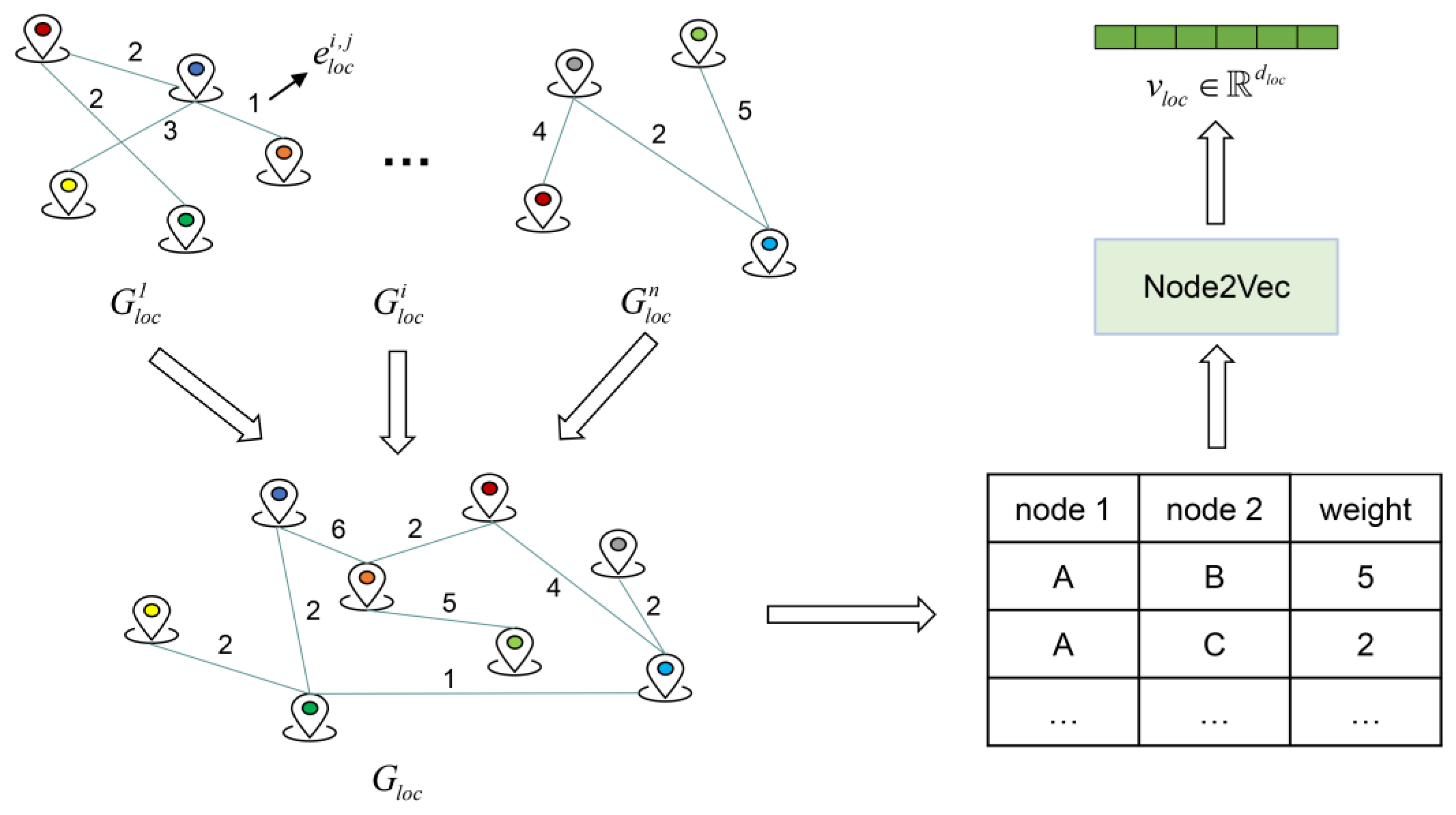
4.1.2. Spatial Interaction Embedding

Trajectory prediction is used to predict future user visits. Thus, correct location information is also critical to the model. Some factors are included in the raw location data, such as location ID, latitude, longitude, and location category information. For example, a location with the ID “49bbd6c0f964a520f4531fe3”, latitude and longitude of 40.719810375488535 and −74.00258103213994, respectively, location category ID “4bf58dd8d48988d127951735”, and category name “Arts & Crafts Store”. The place’s latitude and longitude are directly preserved as its embedding in numerous classic methods for location embedding. Although this strategy is straightforward, the connection between places is overlooked. Indeed, certain venues, such as school buildings and canteens, are extremely likely to be frequented in succession. As a result, the relationship between locations must be carefully considered.

Recent years have seen the application of graph-embedding techniques in a range of domains, including text classification and social influence research. In this research, the graph-embedding technique is used to create location embeddings with full consideration of the transfer relationships between places. The graph-embedding technique is utilized to construct embeddings of locations with full consideration of the transfer link between locations and the degree of transfer potential. Figure 3 depicts how the real behavioral patterns of users are translated into graph structures, considering that a user visited sites A, B, C, D, E, and F in order. These locations are taken as nodes and linked in order, and the location access graph of this user is built.

After the construction of a user’s location graph, all location graphs are built in the same way. The whole location embedding process is displayed in Figure 4.

Then, an undirected weighted location graph $G_{loc}=(V_{loc},E_{loc})$ is constructed, where $V_{loc}$ denotes the collection of all locations and $E_{loc}$ indicates the set of edges. If a person visits two locations adjacent to one another in an unconstrained sequence, there is an edge $e_{loc}^{i,j}$ between location $i$ and location $j$. The trajectory segments of each user are then traversed to obtain the weights of the edges. Then, the weight $w_{loc}^{i,j}$ of the edge $e_{loc}^{i,j}$ is equal to the total number of occurrences of all neighboring location pairs $(lo{c}_i,lo{c}_j)$ or $(lo{c}_{j,}lo{c}_i)$. The graph-embedding technique Node2Vec [29] is used to retrieve the embedding of each graph node, i.e., the embedding vector $v_{loc}\in {ℝ}^{d_{loc}}$ of each location, $d_{loc}$ is the embedding size of the location.

While the location attribute in space has garnered much attention, the location category properties have received less. Location categories are semantically rich spatial information that can be used to analyze movement intentions and patterns. A location category graph $G_{cate}=(V_{cate},E_{cate})$ is generated with a similar method to location embedding. The weights $w_{cate}^{r,s}$ of edges $e_{cate}^{r,s}$ are determined by the number of transfers between the location category $r$ and category $s$. The embedding $v_{cate}\in {ℝ}^{d_{cate}}$ of the location category is acquired by Node2Vec, $d_{cate}$ is the embedding size of the location category.

Then, the embedding $v_p$ of each trajectory point $p$ can be obtained by (1):

$$v_p=v_t\oplus v_{loc}\oplus v_{cate},$$

(1)

where $v_p$ represents the embedding of each location obtained by splicing three embedding vectors $v_t$, $v_{loc}$, and $v_{cate}$, and $\oplus$ denotes the concatenation operation.

4.1.3. Social Relationship Embedding

Each user in the original dataset has a unique ID, which is used to generate the embedding $v_u\in {ℝ}^{d_u}$ of user characteristics in a low-dimensional space of size $d_u$. Then easy differentiation across users is allowed.

Social impacts on mobility behavior have been overlooked because of inadequate consideration of social links. The social relationships between users are represented via a graph in this study. The social user graph $G_{soc}=(V_{soc},E_{soc})$ is constructed using the users’ social connection data, where $V_{soc}$ represents the set of nodes, i.e., users. Similarly, $E_{soc}$ denotes the collection of edges. An edge $e_{soc}^{i,j}$ between a user $i$ and another user $j$ will be generated if they have a link. During the creation process, $V_{soc}\subseteq U$, some users may lack social data, rendering them isolated points in the graph. The Node2Vec algorithm uses other nodes to update the representation of the current node, incorporating social connections between different users. The social embedding is $v_{soc}\in {ℝ}^{d_{soc}}$, the embedding size is $d_{soc}$. Meanwhile, the representation depicts the similarity of social ties. If users’ social connections representation is closer in higher dimensional space, this means that the communities to which they belong are more similar.

The conventional technique of viewing all of a user’s friends equally is abandoned in this work. Because each friend’s effect on a current user’s mobility behavior is often distinct, different influence weights should be considered for different friends. Assume that the user $i$ is the current user, and the set of his friends is expressed as $F_i$, formally donated as $F_i=\{f_1,f_2,\dots ,f_q\}$, where $f_j$ represents the embedding representation vector of the $j$-th friend, and there are $q$ friends in total. Equation (2) can be used to express the impact ${\beta }_{ij}$ of the $j$-th friend on the user $i$ when the influence of various users is considered.

$${\beta }_{ij}=softmax(v_{u_i}\cdot f_j),$$

(2)

where $v_{u_i}$ indicates the representation of the user $i$ and $f_j$ denotes the representation of the user’s $j$-th friend. Their similarity is determined using an inner product, which is then normalized to obtain the degree of effect of the $j$-th friend on the user $i$. The representation of the user $i$’s friends $so{c}_i$ is derived as follows, and the impact of all the user’s friends is considered.

$$so{c}_i={\displaystyle \sum _{j=1}^q{\beta }_{ij}{f}_j}.$$

(3)

As shown in (3), the social relationship representation ${\mathit{soc}}_i$ of the user $i$ is derived through weighted summation. By considering all friends of the current user $i$ and the effect of each friend independently, the ultimate social representation $v_{f_i}$ of the user $i$ is expressed as follows:

$$v_{f_i}=v_{soc}+so{c}_i.$$

(4)

The intermediate representation $v_{soc}$ of the user’s social relationships is produced by graph embedding. $so{c}_i$ indicates the user’s friend representation, which incorporates the diverse effects of various friends using attention.

The embedding representation of the trajectory’s contextual information is gained through the module, which includes temporal information, location information, location category information, and social information. The social representations of the current user’s friends are fused with friend-level attention, which alleviates the problem of social relationships being underrepresented in existing research. Meanwhile, the social relationship representation of the current user is obtained. These embeddings are then fed into the multi-level attention module to improve the learning of trajectory patterns.

4.2. Multi-Level Attention Module

Multi-level attention architecture is proposed to mine individual and group preferences while, simultaneously, user trajectory patterns are learned. The personal preferences of the user are captured through the user-check-in attention layer. Group preferences are reflected through the check-in-level attention layer and the trajectory-level attention layer. A trajectory representation is generated, which incorporates both individual and group preferences. Meanwhile, it alleviates the problem of standard RNN-based models failing to capture the spatial–temporal dependency of lengthy trajectories. Individual preference learning is covered in Section 4.2.1, while group preference learning is discussed in Section 4.2.2.

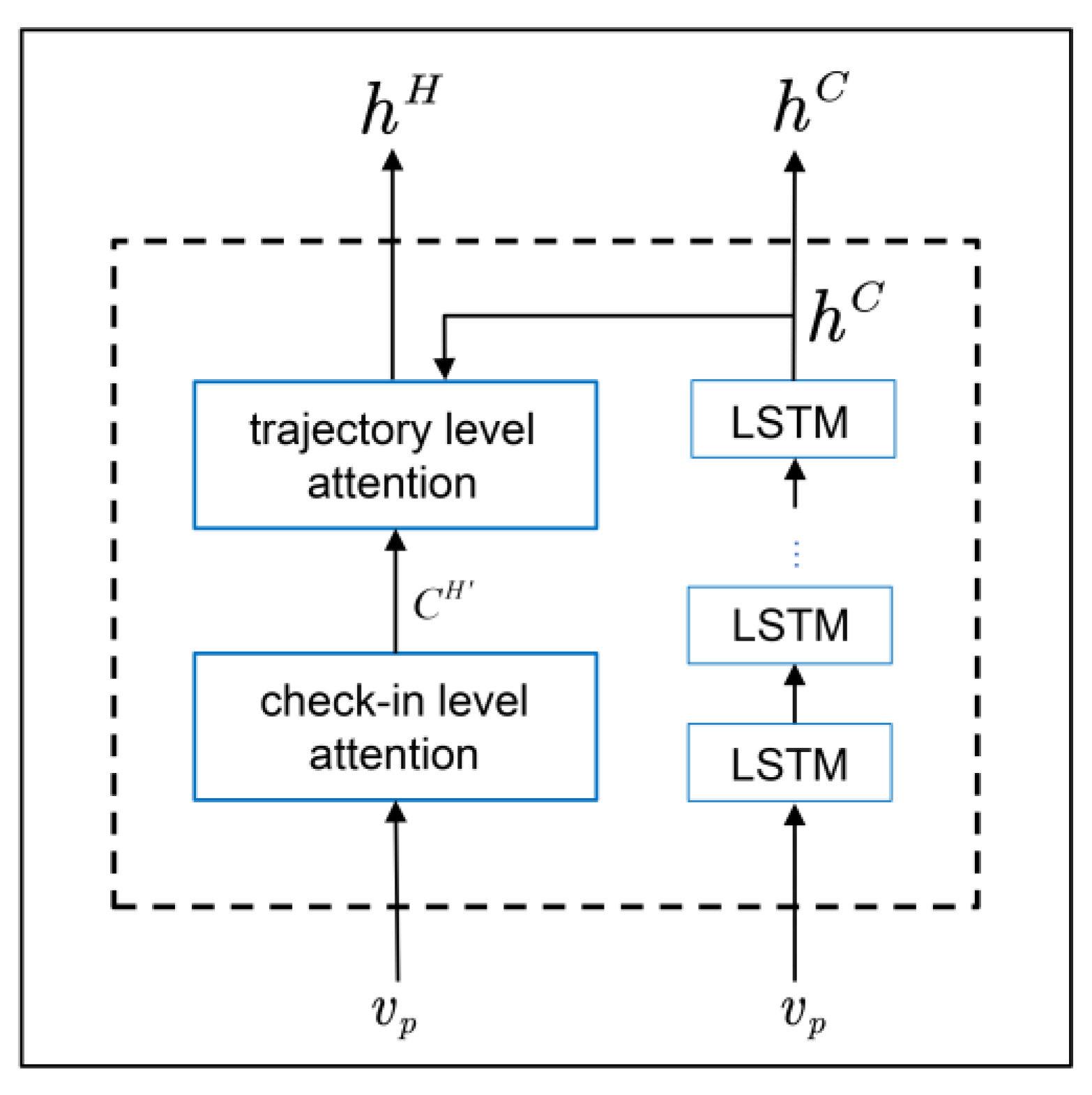
4.2.1. Personal Preference Learning

Individual user travel preferences may be reflected in their historical trajectories. RNNs are frequently used in natural language processing tasks due to their superior ability to process sequences. GRU is a variant of the RNN. User trajectory is a sequence arranged chronologically by trajectory points. Thus, GRU is utilized to deal with user historical trajectories. A user-check-in level attention layer is designed to capture personal preferences for trajectory points, as shown in Figure 5.

As seen in the figure, the trajectory points sequence is fed into the GRU to produce a new trajectory point representation. Through attention, the representation of the user preference for trajectory points is obtained, together with the weight of each point concerning the user representation. Equation (5) can be used to calculate the hidden state $h_i$ of the GRU at the $i$-th time step.

$$h_i=GRU(v_{p_i},h_{i-1}),$$

(5)

where $v_{p_i}$ donates the trajectory point representation vector at the $i$-th time step. $h_{i-1}$ is the hidden state at the $i-1$-th step of GRU.

Although RNNs, especially LSTMs and GRUs, are excellent at capturing short-term dependencies, they are incapable of solving the problem of long-term dependencies. Therefore, the attention mechanism [30] was introduced to enhance the deep neural network’s ability to capture long-term dependencies. It has been applied to a variety of tasks, such as recommendation systems and machine translation. User-check-in attention is designed to learn individual preferences for trajectory points from historical trajectories. The preference score for check-ins at each time step is determined using (6).

$${\alpha }_i=\frac{\mathit{exp}(h_i^T{v}_u)}{{\displaystyle {\sum }_{i=1}\mathit{exp}(h_i^T{v}_u)}}.$$

(6)

The user’s preference representation $p_u$ is obtained by weighting the sum of the user’s preference scores for each time step’s check-in. It can be expressed as follows:

$$p_u={\displaystyle \sum {\alpha }_i}{h}_i,$$

(7)

And the representation $p_u$ is utilized to reveal the individual user’s preference for trajectory points.

4.2.2. Group Preference Learning

In addition to personal preferences, users’ travel decisions are influenced by group preferences. In this study, group preferences are learned through the check-in-level attention layer and the trajectory-level attention layer.

The interaction between check-ins has not been fully considered in previous studies, which neglects the fact that one location has an impact on the frequency of check-ins at nearby locations. For instance, there are generally several restaurants located near a park, and the number of patrons at these restaurants is influenced by the park’s people flow. A check-in-level attention scheme is proposed to obtain a historical trajectory representation that considers the location interactions. Meanwhile, the spatial–temporal dependencies of lengthy trajectories are captured. The different influences of historical trajectories on current trajectories are considered in the trajectory-level attention layer. The group preference learning scheme is displayed in Figure 6.

For the historical trajectory $T_u^H$ of the user $u$, the interactions between check-ins are considered and the critical information in the trajectory is captured by the trajectory itself. A multi-head self-attention [30] is first used to obtain the updated representation of each trajectory point. The trajectory representation is then updated via other layers in the check-in level attention layer, which is illustrated in Figure 7.

The check-in embedding vector obtained by the embedding module is passed to the multi-head attention sublayer. Unlike standard RNNs that have inherent orderliness, all time steps are accepted concurrently in this structure, which sacrifices orderliness between check-ins but gains parallelism. As a result, the position encoding [30], which is computed in (8) and (9), must be included to obtain the sequence.

$$pos\_emb(pos,2i)=\mathit{sin}(pos/{10000}^{2i/d}),$$

(8)

$$pos\_emb(pos,2i+1)=cos(pos/{10000}^{2i/d}),$$

(9)

where $pos$ indicates the position of the check-in point in the trajectory, $i$ denotes the position of the check-in embedding, and $d$ represents the dimension of the position embedding. The output is defined as $v_{pos}$. By position embedding, the relative position information between the trajectory points is stored in the trajectory representation. The position embedding and the trajectory point embedding are then passed into the multi-head self-attention, as specified in (10).

$$x=v_p+v_{pos}.$$

(10)

Here, $x$ represents the input of the multi-head self-attention. Numerous trajectory points are then supplied into the multi-head attention layer. When the attention score $S$ is utilized as the query vector, the relevance of other locations relative to the current location can be conveyed. The weight of each location’s vector in the final historical trajectory context vector is determined by expressing the similarity between two locations. The attention score $S$ is calculated by (11), and it is then normalized using (12) to produce the normalized attention score $a_{ij}$.

$$S_{ij}=\frac{Q\cdot K^T}{\sqrt{d_k}},$$

(11)

$$a_{ij}=\frac{\mathit{exp}(S_{ij})}{{\displaystyle {\sum }_{k=1}^n\mathit{exp}(S_{ik})}},$$

(12)

where $d_k$ is a scaling factor that is used for normalization, which is used to ensure the gradient remains steady during the training process. The $Q\in R^{M\times d}$, $K\in R^{N\times d}$, and $V\in R^{N\times d}$ are matrices gained by performing various linear transformations on the matrix $X$ composed of vectors $x$, respectively. The formulas are as follows:

$$Q=X\cdot W_Q,$$

(13)

$$K=X\cdot W_K,$$

(14)

$$V=X\cdot W_V.$$

(15)

After the attention score $a_{ij}$ is obtained, the weighted sum can be computed with the score and value matrix $V$. As indicated in (16), the final trajectory context $C^H$ is the weighted sum of each check-in vector.

$$C^H={\displaystyle \sum _{i=1}^n{a}_i}V.$$

(16)

Multi-head attention maps $Q$ and $K$ to different subspaces $({\gamma }_1,{\gamma }_{2,}\dots ,{\gamma }_h)$ of the high-dimensional space $\gamma$ to compute the similarity, which enhances the expressiveness of each attention layer without increasing the number of parameters. The attention information from multiple subspaces is then combined, which lowers the dimension used to compute each head’s attention and prevents overfitting. Because distinct distributions are included in attention in different spaces, the similarities between different locations from several perspectives can be evaluated by multi-head attention. The results of all views are then combined to provide a contextual representation $C^{H^{\prime }}$ of historical trajectories, which is shown in (17):

$$C^{H^{\prime }}=(C_1^H\oplus C_2^H\oplus \cdots \oplus C_h^H)\cdot W_H,$$

(17)

where $h$ specifies the number of heads, and $\oplus$ represents the concatenation operation. $C_i^H$ is the context representation of the $i$-th space, and $W_H$ is the weight matrix.

After the intermediate trajectory representation $C^{H^{\prime }}$ is obtained, the representation is supplied into the feed-forward layer for spatial transformation. ReLu is the activation function, and two linear transformation layers are included in the layer. The output space of the attention is transformedby the nonlinear transformation. Therefore, the expressiveness of the model is enhanced by the space transformation.

LSTM can obtain a hidden representation of an input sequence. For the current trajectory, the representation $h^C$ is obtained using LSTM, as indicated in (18):

$$h_i^C=LSTM(v_p,h_{i-1}).$$

(18)

The similarity of all historical trajectories to the current trajectory $h^C$ is then computed utilizing trajectory-level attention. The formula is as follows.

$${\alpha }_i=\frac{\mathit{exp}(h^C{C}_i^{H^{\prime }})}{{\displaystyle {\sum }_{j=1}\mathit{exp}(h^C{C}_j^{H^{\prime }})}}.$$

(19)

After the similarity score ${\alpha }_i$ is acquired, the ultimate representation $h^H$ of the historical trajectory context is obtained by summing all historical trajectories according to their weights, as expressed in (20):

$$h^H={\displaystyle \sum {\alpha }_i{C}_i^{H^{\prime }}}.$$

(20)

The multi-level attention module consists of three attention layers, which are the user-check-in attention, check-in-level attention, and trajectory-level attention layers. Additionally, the user personal preference representation $p_u$ for trajectory point, historical group preference representation $h^H$, and current group preference representation $h^C$ are collected. Specifically, the GRU and the user-check-in attention layers are used to determine the user’s personal preferences for trajectory points. The group preference representation $h^H$ and $h^C$ are gained by the check-in-level attention layer and the trajectory-level attention layer. After a final trajectory representation that incorporates personal preferences and group preferences is obtained, the representation is passed to the trajectory prediction module for trajectory prediction.

4.3. Trajectory Prediction Module

The model architecture concludes with the prediction module. The component consists of three layers, which are composed of a concatenation layer, a fully connected layer, and a normalization layer.

Five representation vectors are joined to produce the ultimate trajectory representation via the concatenation layer, which are the user’s representation $v_u$, the social representation $v_{f_i}$, the user’s personal preference representation $p_u$ for the trajectory point, the historical representation $h^H$ of group preference, and the current representation $h^C$ of group preference. Personal preference is composed of users’ features $v_u$, social preferences $v_{f_i}$, and preferences $p_u$ for trajectory points. Group preference is constructed by historical preference $h^H$ and current preference $h^C$. The user’s next check-in is then determined using a linear transformation and the possibility of each location. Eventually, the possibility is converted into a probability of check-in by the normalization layer. The calculation formula is presented in (21).

$$y_u^k=soft\mathit{max}(W_u\cdot (v_u\oplus v_{f_i}\oplus p_u\oplus h^H\oplus h^C)+b_u),$$

(21)

where $W_u$ and $b_u$ are the weight matrix and bias term, respectively. The output $y_u^k$ of the model represents the probability of the user’s next check-in location within the $k$-th trajectory segment. The corresponding location of the highest probability is chosen as the user’s next predicted trajectory point.

4.4. Trajectory Prediction Algorithm and Model Training

A trajectory prediction algorithm is proposed with the three previously mentioned modules as well as data preprocessing in this paper. The details are shown in Algorithm 1.

Algorithm 1. Multi-level attentive context-aware trajectory prediction algorithm for mobile social users.

Input: Preprocessed user trajectory data Output: List of predicted locations

List of predicted locations $R$ = $\varnothing$. Construct the location graph $G_{loc}$, the location category graph $G_{cate}$, and the user social graph $G_{soc}$. Use Node2Vec to obtain the location embedding $v_{loc}$, the location category embedding $v_{cate}$, and the social embedding $v_{soc}$. For a user $i$ in the set $U$ of users:  Get user feature embedding $v_u$ and temporal embedding $v_t$ based on the user $i$’s ID and temporal data in the trajectory.  Obtain embedding $v_p$ of trajectory point $p$ by (1), getting the history trajectory representation $H$ and current trajectory representation $C$.  Get the user $i$’s personal social preference $v_{f_i}$ by (2)~(4).  Get the user $i$’s personal trajectory point preference $p_u$ by (5)~(7).  For trajectory segment $j$ in the set of trajectory segments of the user $i$:   Divide the training set and test set by 8:2.  End for  For the current trajectory $C$, get the representation $h^C$ by (18).  For the history trajectory $H$, get the intermediate representation $C^{H^{\prime }}$ with check-ins interactions by (8)~(17).  Gain the ultimate history trajectory representation $h^H$ by fusing the history trajectory according to the importance to the current trajectory by (19) and (20).  Obtain the current user $i$’s prediction result by (21). End for Train the model according to the cross-entropy loss. Feed the test data into the trained model to obtain the prediction results, and then add them to the result list $R$. Return the result list $R$.

The location graph $G_{loc}$, the location category graph $G_{cate}$, and the user social graph $G_{soc}$ are created first. Then, using various embedding approaches, location embedding $v_{loc}$, location category embedding $v_{cate}$, and users’ social interaction embedding $v_{soc}$ are obtained. The embedding of user characteristics $v_u$ and time $v_t$ is generated by the user ID and check-in time. Personal social preference $v_{f_i}$ is gained by friend-level attention. Each user’s trajectory segments are separated into a training set and a test set. The former is separated into two parts: historical and current trajectory segments. For the current trajectory, its representation $h^C$ is obtained by LSTM, while the user historical trajectory context $h^H$ is obtained via the check-in-level attention and the trajectory-level attention. The interactions of check-ins and the historical group preferences are all contained in $h^H$. Finally, the prediction is made with the help of the prediction module.

5. Experiments

The experimental design and results are presented in this section to validate the performance of the proposed model MACTP. The dataset and assessment criteria are supplied first, followed by the comparison methods. Finally, the experimental results and analysis are displayed.

5.1. Datasets and Data Preprocessing

The proposed model was validated using the following datasets.

Foursquare. This was collected from a mobile social network application Foursquare. The experiments in this study were conducted using check-in data from one of the cities, New York City (NYC). The dataset was named Foursquare–NYC. Foursquare contains 227,428 user check-in records. Each check-in record contains the user id, timestamp, location id, location latitude, location longitude, location category id, and location category.

Gowalla. This dataset was collected from the Gowalla website. It contains 6,442,890 check-in records. This dataset contains two sub-datasets: the check-in dataset and the social dataset. In the check-in dataset, each record contains the user ID, time, location ID, and the longitude and latitude of the location. Each record of the social dataset represents a set of connections with the data format (first user ID, second user ID). In this research, Los Angeles (LA) and Houston were selected as the experimental datasets by the Ray method. The corresponding datasets were named Gowalla–LA and Gowalla–Houston.

The following steps were performed on the Foursquare dataset to generate the final trajectory segments. Firstly, users and locations that are infrequently visited are deleted, i.e., users who check in to fewer than ten different locations, as well as places that have been visited fewer than ten times. Then, each user’s trajectories are built in chronological order. If a user’s trajectory length is shorter than eight, the user’s data are deleted to improve prediction performance. The trajectory segments are created based on the defined window size, which is 48 h in this case. Finally, any trajectory segments with fewer than two trajectory points are removed. These steps yield the processed trajectory data.

The statistics of the datasets are shown in

Table 1. Statistics of the dataset.

Dataset	The No. of Users	The No. of Locations	Locs./Users.
Gowalla–LA	1057	10,657	10.08
Gowalla–Houston	821	10,282	12.52
Foursquare–NYC	1082	34,440	31.83

. Each dataset was divided into a training set and a test set based on users. The earlier 80% of each user’s trajectories were utilized as the training data and the latter 20% as the test data in the experiment.

5.2. Evaluation Metrics

The model performance is evaluated by utilizing commonly used performance metrics including accuracy and normalized discounted cumulative gain (NDCG).

The accuracy $Acc@k$ can be defined according to (22).

$$Acc@k=\frac{1}{\left|m-1\right|}{\displaystyle \sum _{t=2}^m(lo{c}_t}\in R_t(k)).$$

(22)

If the true location $lo{c}_t$ appears in the list $R_t(k)$ of the predicted top -$k$ results, the user’s check-in location will be successfully predicted. The value of $lo{c}_t\in R_t(k)$ is 1 in this case, otherwise, it is 0. $m$ is the number of locations in the historical trajectory.

NDCG is another evaluation metric. When there is a high degree of correlation between results at more advanced positions, the metric will be increased. The formula is shown in (23).

$$NDCG@k=\frac{1}{z}{\displaystyle \sum _{i=1}^k\frac{2^{idx(R(i)\cap R^{\prime })}-1}{{\mathit{log}}_2(i+1)}},$$

(23)

where $z$ is a normalization constant, $R(i)$ refers to the $i$-th predicted location in the list of the top -$k$ predicted locations, and $R^{\prime }$ represents the test set’s list of locations. The $idx(·)$ is the index function.

5.3. Baselines

The proposed model MACTP was compared to several approaches to assess its effectiveness. Both classical and deep neural-network-based trajectory prediction methods were included.

Markov [5]. It is extensively used in the prediction of human trajectories. The first-order transfer probability between check-ins is encoded in a transfer probability matrix, and the likelihood that a user will visit a place is calculated using the user’s previous visits and the transfer probability matrix.

RNN-Short. This is a variant of STRNN [31], in which trajectories of the model are fed daily trajectories rather than continuous spatial–temporal data.

RNN-Long. This is a variation of STRNN [31], where the RNN-based model is GRU and the model is directly fed one-month trajectories. It is no longer capable of modeling continuous spatial–temporal data.

DeepMove [8]. This is a method based on attention mechanisms and neural networks that learns users’ periodic movement patterns and preferences using historical and recent trajectories.

PLSPL [32]. This is a method for the next location recommendation. It models users’ long- and short-term preferences to learn different dependencies for different users. Locations and the categories of locations are considered to better determine where a user will go next.

MACTP. This is the model proposed in this study, which incorporates a range of contextual factors such as information about temporal, spatial, social, and location categories. A multi-level attention module is used to mine users’ individual and group preferences for trajectory prediction.

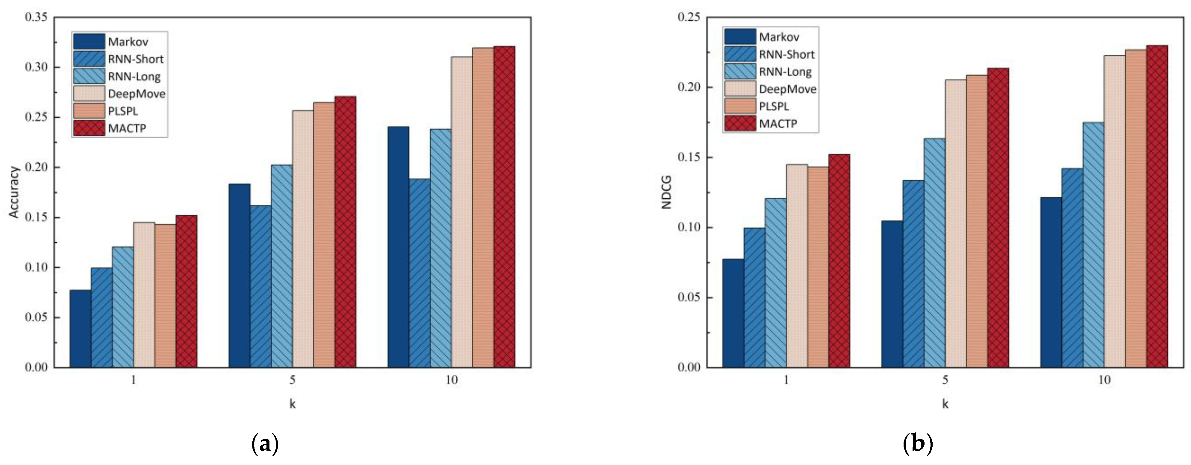
5.4. Method Comparison

The experimental results of the trajectory prediction task on the Gowalla–LA, Gowalla–Houston, and Foursquare–NYC datasets are shown in

Table 2. Methods’ comparison results on Gowalla–LA.

Methods	Acc@1	Acc@5	Acc@10	NDCG@1	NDCG@5	NDCG@10
Markov	0.0774	0.1833	0.2405	0.0774	0.1047	0.1214
RNN-Short	0.0996	0.1619	0.1883	0.0996	0.1336	0.1420
RNN-Long	0.1206	0.2024	0.2383	0.1206	0.1634	0.1749
DeepMove	0.1449	0.2567	0.3103	0.1449	0.2052	0.2225
PLSPL	0.1431	0.2648	0.3194	0.1431	0.2087	0.2267
MACTP	0.1521	0.2707	0.3209	0.1521	0.2136	0.2298

,

Table 3. Methods’ comparison results on Gowalla–Houston.

Methods	Acc@1	Acc@5	Acc@10	NDCG@1	NDCG@5	NDCG@10
Markov	0.1114	0.2095	0.2470	0.1114	0.1189	0.1246
RNN-Short	0.1066	0.1745	0.1966	0.1066	0.1417	0.1487
RNN-Long	0.1249	0.2115	0.2514	0.1249	0.1702	0.1830
DeepMove	0.1437	0.2492	0.2939	0.1437	0.1998	0.2142
PLSPL	0.1404	0.2531	0.3026	0.1404	0.2013	0.2183
MACTP	0.1613	0.2744	0.3266	0.1613	0.2198	0.2367

, and

Table 4. Methods’ comparison results on Foursquare–NYC.

Methods	Acc@1	Acc@5	Acc@10	NDCG@1	NDCG@5	NDCG@10
Markov	0.1228	0.2526	0.3178	0.1228	0.1204	0.1141
RNN-Short	0.0976	0.1951	0.2262	0.0976	0.1495	0.1596
RNN-Long	0.1179	0.2374	0.2758	0.1179	0.1817	0.1942
DeepMove	0.1453	0.2756	0.3087	0.1453	0.2159	0.2267
PLSPL	0.1468	0.2937	0.3349	0.1468	0.2203	0.2358
MACTP	0.1653	0.3445	0.4062	0.1653	0.2584	0.2784

, respectively.

The accuracy and NDCG for all comparison methods on the three datasets are displayed in Figure 8, Figure 9 and Figure 10. The results for Acc@1, Acc@5, and Acc@10 are shown in Figure 8a, Figure 9a, and Figure 10a, respectively. The results for NDCG@1, NDCG@5, and NDCG@10 are shown in Figure 8b, Figure 9b and Figure 10b, respectively.

The same method produces different results on different datasets, which is demonstrated in Figure 8, Figure 9 and Figure 10, owing primarily to the size disparities across the datasets. The sizes of the datasets used in this paper are Gowalla–LA < Gowalla–Houston < Foursquare–NYC, and their performance using the same approach follows the same trend, indicating that data sparsity is a significant determinant of prediction accuracy.

From an overall perspective, RNN-Short performs the worst in terms of accuracy. One limitation is that it only considers temporal and spatial factors; the other is that the model’s input is daily trajectory data with low coherence of historical data. On NDCG, Markov performs poorly because it solely analyzes first-order transfer probabilities. Both in terms of accuracy and NDCG, RNN-Long outperforms Markov and RNN-Short. In comparison to RNN-Short, it inputs historical trajectories that are continuous for one month, which mines the user behavior patterns in historical trajectories more thoroughly. When compared to Markov, it considers not only the location transfer but also time and space. RNN-Long, on the other hand, simply takes the current trajectory into account and does not mine for patterns in the historical trajectory, which is why DeepMove and PLSPL outperform it.

In comparison to the above methods, MACTP incorporates social relationships and captures the spatial–temporal dependency of lengthy trajectories using multi-level attention. MACTP’s superior results imply that social relationships are helpful for trajectory prediction and that weighting of current users’ friends can produce more accurate results than previous methods. Meanwhile, check-in level attention and trajectory-level attention account for the impact of historical trajectories on current trajectories, which increases the expressiveness of the model. When compared to the methods mentioned previously, it can be observed that the proposed model performs better at prediction.

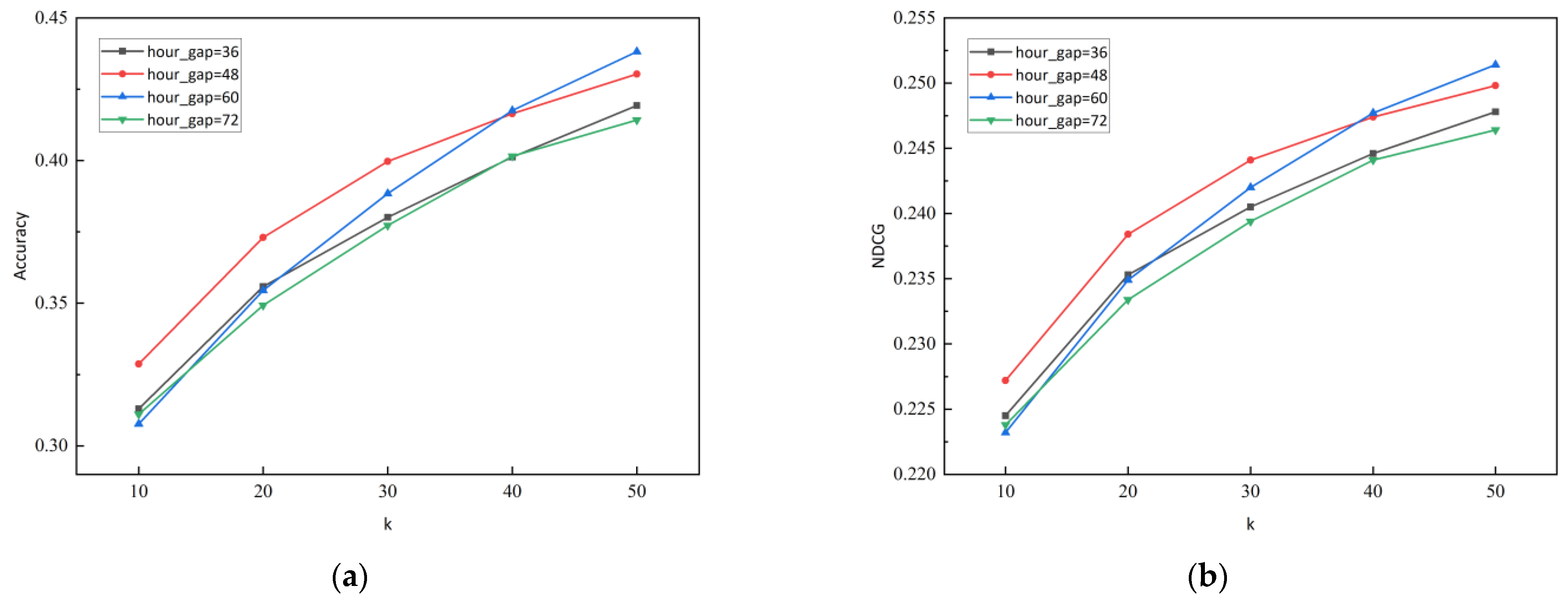
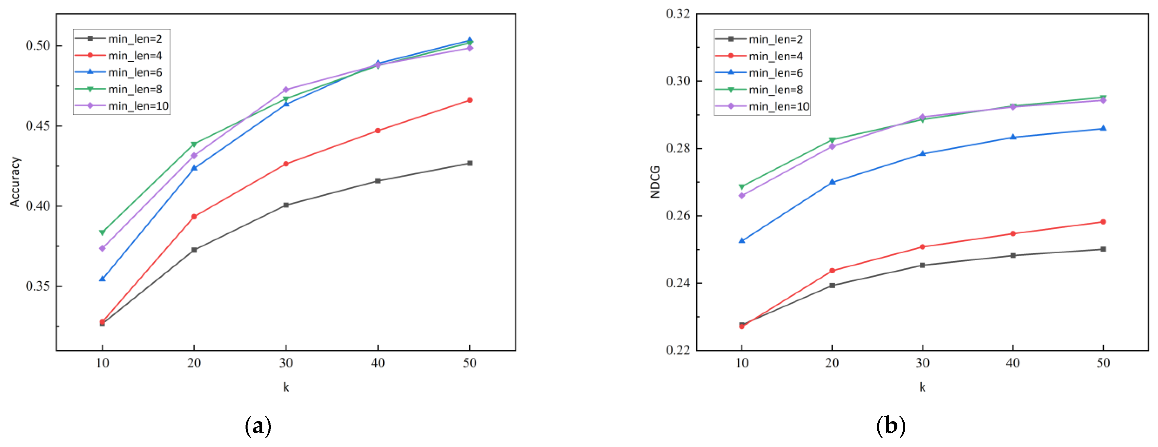
5.5. Hyperparameter Settings

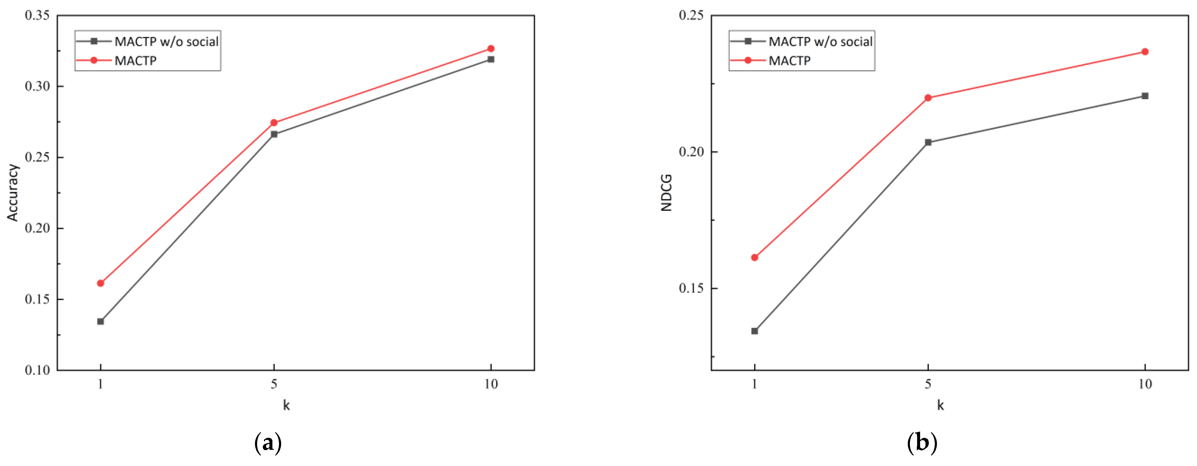
It was studied how specific hyperparameters, such as time intervals and the minimum length of trajectory segments, affect the model’s performance.

First, for the time interval, we set the starting time interval for separating the trajectory segments to 36. The values of $\mathit{hour}\_gap$ were then set to 36, 48, 60, and 72. The prediction list had lengths $k$ of 10, 20, 30, 40, and 50. The results of the accuracy and NDCG are shown in Figure 11.

As can be observed from the figure, evaluation metrics of the model first rise as $\mathit{hour}\_gap$ grows, and when $\mathit{hour}\_gap=48$, the model’s performance declines as it continues to increase. The temporal relevance of user behavior inside a trajectory segment is determined by the time interval parameter. When it takes a small value, the temporal continuity of user behavior reduces, and when it takes a value above a certain threshold, it leads to a decline in the temporal correlation of user behavior, resulting in reduced accuracy and NDCG. The time interval is set at 48.

Next, the impact of the trajectory segment’s minimum length $\mathit{min}\_len$ on the model is examined. The size of $\mathit{min}\_len$ ranges from 2 to 10, with a step size of 2. The experimental results are displayed in Figure 12.

As seen in Figure 12, the values of the accuracy and NDCG increase as $k$ grows. The optimal results are achieved at $k=10$ and $k=20$ when $\mathit{min}\_len=8$. Nonetheless, the performance of the model is greater for $\mathit{min}\_len=10$ while increasing $k$. In location prediction, the larger the length of the prediction list, the more choices the user has, but too large a value of $k$ can make the users’ choices difficult. In this study, when picking hyperparameters, we chose to utilize the results with small $k$ as a reference. The value of $\mathit{min}\_len$ was set to 8 in the experiment.

In the model, the embedding dimension of the location is set to be $d_{loc}=500$, the social embedding size to be $d_{soc}=40$, the location category embedding size to be $d_{cate}=50$, and the time embedding size to be $d_t=10$. The head number of the multi-head attention is configured to be 2. The hidden size of LSTM is set to 560. The hidden size of GRU is set to 280. Cross-entropy loss is employed as the loss function. All parameters are subjected to L2 regularization. The learning rate is 0.0001. All fully connected layers are processed using the dropout strategy, which avoids overfitting, and the dropout rate is set to be 0.3.

5.6. Ablation Study

A variant of MACTP was conducted on both Gowalla–LA and Gowalla–Houston to verify the effectiveness of the social relationship submodule. The Foursquare dataset was not considered in this experiment due to the absence of social relationship data. The model without the social attention submodule is denoted as “MACTP w/o social” in this work, while “MACTP” refers to the entire model. The results of the $Acc@k$ and $NDCG@k$ are displayed in Figure 13 and Figure 14, where $k$ is 1, 5, and 10.

As shown in Figure 13 and Figure 14, from accuracy and NDCG, the performance of the model “MACTP w/o social” without the social attention submodule is lower than that of the whole model “MACTP”, indicating that the model that considers social interactions has superior prediction performance, and the social submodule is effective. Because influence among friends tends to have a strong impact on users’ travel decisions, the experimental results are also consistent with intuitive ideas in everyday life.

6. Conclusions

Trajectory prediction of humans is an important task. However, trajectory context has not been fully considered in prior research, and spatial–temporal dependence of long trajectories is difficult to characterize. A multi-level attentive context-aware model, “MACTP”, for predicting the check-in locations of mobile social users is proposed in this paper. The experiments show that the proposed model alleviates these problems and significantly improves human trajectory prediction performance.

Along with the trajectory’s temporal and spatial information, the embedding module incorporates social data and location category information via various methods to enrich the trajectory’s context. Both individual and group preferences are considered in the trajectory representation. In terms of individual preference, the social preference representation and location preference representation of users are generated by friend-level attention and user-check-in level attention. The acquisition of group preference is mainly related to check-in-level attention and trajectory-level attention. The initial representation of historical trajectories is obtained through check-in-level attention. The representation of current trajectories is gained through LSTM. The representation of historical trajectories with the consideration of current trajectories is obtained by check-in level attention. In this way, personal preference is represented by users’ social preference and trajectory point preference. Group preference is captured by long-term preference from historical trajectories and short-term preference from current trajectories. The ultimate trajectory representation is then gained by combining these representations. Finally, a prediction of the location is made. The results of the three datasets indicate that the proposed model improves the performance of trajectory prediction.

There are some limitations to this study. Some LBSN datasets contain user comment data, which are not considered in the current model. The trajectory prediction performance is not stable on different datasets, which can be found in the experiment results. In the future, user textual comment data will be incorporated into the model, and data augmentation will be explored to enrich trajectory representation and improve the robustness of the model.

References

1. Liu, Y.; Pham, T.-A.; Cong, G.; Yuan, Q. An experimental evaluation of point-of-interest recommendation in location-based social networks. In Proceedings of the VLDB Endowment; VLDB Endowment: Sydney, Australia, 2017; pp. 1010–1021. [Google Scholar]
2. Liu, Q.; Zuo, Y.; Yu, X.; Chen, M. TTDM: A travel time difference model for next location prediction. In Proceedings of the 2019 20th IEEE International Conference on Mobile Data Management (MDM), Hong Kong, China, 10–13 June 2019; pp. 216–225. [Google Scholar]
3. Liu, C.H.; Wang, Y.; Piao, C.; Dai, Z.; Yuan, Y.; Wang, G.; Wu, D. Time-aware location prediction by convolutional area-of-interest modeling and memory-augmented attentive LSTM. IEEE Trans. Knowl. Data Eng. 2022, 34, 2472–2484. [Google Scholar] [CrossRef]
4. Bao, Y.; Huang, Z.; Li, L.; Wang, Y.; Liu, Y. A BiLSTM-CNN model for predicting users’ next locations based on geotagged social media. Int. J. Geogr. Inf. Sci. 2020, 35, 639–660. [Google Scholar]
5. Yang, D.; Li, B.; Cudré-Mauroux, P. Poisketch: Semantic place labeling over user activity streams. In Proceedings of the Twenty-Fifth International Joint Conference on Artificial Intelligence (IJCAI), New York, NY, USA, 9–15 July 2016; pp. 2697–2703. [Google Scholar]
6. Yang, D.; Zhang, D.; Zheng, V.W.; Yu, Z. Modeling user activity preference by leveraging user spatial temporal characteristics in LBSNs. IEEE Trans. Syst. Man Cybern. Syst. 2015, 45, 129–142. [Google Scholar] [CrossRef]
7. Mathew, W.; Raposo, R.; Martins, B. Predicting future locations with hidden Markov models. In Proceedings of the 2012 ACM Conference on Ubiquitous Computing, Pittsburgh, PA, USA, 5–8 September 2012; pp. 911–918. [Google Scholar]
8. Feng, J.; Li, Y.; Zhang, C.; Sun, F.; Meng, F.; Guo, A.; Jin, D. Deepmove: Predicting human mobility with attentional recurrent networks. In Proceedings of the 2018 World Wide Web Conference on World Wide Web—WWW ‘18, Lyon, France, 23–27 April 2018; pp. 1459–1468. [Google Scholar]
9. Li, J.; Wang, Y.; McAuley, J. Time interval aware self-attention for sequential recommendation. In Proceedings of the 13th International Conference on Web Search and Data Mining, Houston, TX, USA, 3–7 February 2020; pp. 322–330. [Google Scholar]
10. Zhao, P.; Luo, A.; Liu, Y.; Zhuang, F.; Xu, J.; Li, Z.; Zhou, X. Where to go next: A spatio-temporal gated network for next poi recommendation. IEEE Trans. Knowl. Data Eng. 2022, 34, 2512–2524. [Google Scholar] [CrossRef]
11. Martin, H.; Bucher, D.; Suel, E.; Zhao, P.; Perez-Cruz, F.; Raubal, M. Graph convolutional neural networks for human activity purpose imputation from GPS-based trajectory data. In Proceedings of the NIPS Spatiotemporal Workshop at the 32nd Annual Conference on Neural Information Processing Systems, Montréal, QC, Canada, 3–8 December 2018. [Google Scholar]
12. Tang, J.; Wang, K. Personalized top-n sequential recommendation via convolutional sequence embedding. In Proceedings of the Eleventh ACM International Conference on Web Search and Data Mining, Marina del Rey, LA, USA, 5–9 February 2018; pp. 565–573. [Google Scholar]
13. Yao, D.; Zhang, C.; Huang, J.; Bi, J. Serm: A recurrent model for next location prediction in semantic trajectories. In Proceedings of the 2017 ACM on Conference on Information and Knowledge Management, Singapore, 6–10 November 2017; pp. 2411–2414. [Google Scholar]
14. Li, M.; Lu, F.; Zhang, H.; Chen, J. Predicting future locations of moving objects with deep fuzzy-LSTM networks. Transp. A 2018, 16, 119–136. [Google Scholar] [CrossRef]
15. Zhang, X.; Li, B.; Song, C.; Huang, Z.; Li, Y. SASRM: A semantic and attention spatio-temporal recurrent model for next location prediction. In Proceedings of the 2020 International Joint Conference on Neural Networks (IJCNN), Glasgow, UK, 19–24 July 2020; pp. 1–8. [Google Scholar]
16. Guo, Q.; Sun, Z.; Zhang, J.; Theng, Y.L. An attentional recurrent neural network for personalized next location recommendation. In Proceedings of the AAAI Conference on Artificial Intelligence, New York, NY, USA, 7–20 February 2020; pp. 83–90. [Google Scholar]
17. Sun, K.; Qian, T.; Chen, T.; Liang, Y.; Nguyen, Q.-V.H.; Yin, H. Where to go next: Modeling long-and short-term user preferences for point-of-interest recommendation. In Proceedings of the AAAI Conference on Artificial Intelligence, New York, NY, USA, 7–20 February 2020; pp. 214–221. [Google Scholar]
18. Liang, W.; Zhang, W. Learning social relations and spatiotemporal trajectories for next check-in inference. IEEE Trans. Neural Netw. Learn. Syst. 2020, 34, 1789–1799. [Google Scholar] [CrossRef] [PubMed]
19. Liu, J.; Chen, Y.; Huang, X.; Li, J.; Min, G. GNN-based long and short term preference modeling for next-location prediction. Inform. Sci. 2023, 629, 1–14. [Google Scholar] [CrossRef]
20. Liu, A.; Zhang, Y.; Zhang, X.; Liu, G.; Zhang, Y.; Li, Z.; Zhao, L.; Li, Q.; Zhou, X. Representation learning with multi-level attention for activity trajectory similarity computation. IEEE Trans. Knowl. Data Eng. 2022, 34, 2387–2400. [Google Scholar] [CrossRef]
21. Wang, S.; Li, A.; Xie, S.; Li, W.; Wang, B.; Yao, S.; Asif, M.; Xia, M. A spatial-temporal self-attention network (STSAN) for location prediction. Complexity 2021, 2021, 6692313. [Google Scholar] [CrossRef]
22. Abideen, Z.U.; Sun, H.; Yang, Z.; Ahmad, R.Z.; Iftekhar, A.; Ali, A. Deep wide spatial-temporal based transformer networks modeling for the next destination according to the taxi driver behavior prediction. Appl. Sci. 2021, 11, 17. [Google Scholar] [CrossRef]
23. Zhong, T.; Zhang, S.; Zhou, F.; Zhang, K.; Trajcevski, G.; Wu, J. Hybrid graph convolutional networks with multi-head attention for location recommendation. World Wide Web 2020, 23, 3125–3151. [Google Scholar] [CrossRef]
24. Wu, J.; Hu, R.; Li, D.; Ren, L.; Hu, W.; Xiao, Y. Where have you been: Dual spatiotemporal-aware user mobility modeling for missing check-in POI identification. Inform. Process. Manag. 2022, 59, 103030. [Google Scholar] [CrossRef]
25. Fang, J.; Meng, X.; Qi, X. A top-k POI recommendation approach based on LBSN and multi-graph fusion. Neurocomputing 2023, 518, 219–230. [Google Scholar] [CrossRef]
26. Fang, J.; Meng, X. URPI-GRU: An approach of next POI recommendation based on user relationship and preference information. Knowl. Based Syst. 2022, 256, 109848. [Google Scholar] [CrossRef]
27. Gao, Q.; Zhou, F.; Zhong, T.; Trajcevski, G.; Yang, X.; Li, T. Contextual spatio-temporal graph representation learning for reinforced human mobility mining. Inform. Sci. 2022, 606, 230–249. [Google Scholar] [CrossRef]
28. Feng, J.; Li, Y.; Yang, Z.; Qiu, Q.; Jin, D. Predicting human mobility with semantic motivation via multi-task attentional recurrent networks. IEEE Trans. Knowl. Data Eng. 2022, 34, 2360–2374. [Google Scholar] [CrossRef]
29. Grover, A.; Leskovec, J. Node2vec: Scalable feature learning for networks. In Proceedings of the 22nd ACM SIGKDD International Conference on Knowledge Discovery and Data Mining, San Francisco, CA, USA, 13–17 August 2016; pp. 855–864. [Google Scholar]
30. Vaswani, A.; Shazeer, N.; Parmar, N.; Uszkoreit, J.; Jones, L.; Gomez, A.N.; Kaiser, Ł. Attention is all you need. In Proceedings of the Advances in Neural Information Processing Systems 30: Annual Conference on Neural Information Processing Systems 2017, Long Beach, CA, USA, 4–7 December 2017; pp. 5998–6008. [Google Scholar]
31. Liu, Q.; Wu, S.; Wang, L.; Tan, T. Predicting the next location: A recurrent model with spatial and temporal contexts. In Proceedings of the Thirtieth AAAI Conference on Artificial Intelligence, Phoenix, AZ, USA, 12–17 February 2016; pp. 194–200. [Google Scholar]
32. Wu, Y.; Li, K.; Zhao, G.; Qian, X. Personalized long-and short-term preference learning for next POI recommendation. IEEE Trans. Knowl. Data Eng. 2022, 34, 1944–1957. [Google Scholar] [CrossRef]
Figure 1. The framework of the trajectory prediction model.
Electronics 12 02240 g001
Figure 2. An example of time embedding.
Electronics 12 02240 g002
Figure 3. The construction of a user’s location graph.
Electronics 12 02240 g003
Figure 4. The process of location embedding.
Electronics 12 02240 g004
Figure 5. User-check-in attention.
Electronics 12 02240 g005
Figure 6. The scheme of group preference learning.
Electronics 12 02240 g006
Figure 7. The structure of check-in level attention.
Electronics 12 02240 g007
Figure 8. Results of methods on Gowalla–LA dataset. (a) Accuracy of the methods; (b) NDCG of the methods.
Electronics 12 02240 g008
Figure 9. Results of methods on Gowalla–Houston dataset. (a) Accuracy of the methods; (b) NDCG of the methods.
Electronics 12 02240 g009
Figure 10. Results of methods on Foursquare–NYC dataset. (a) Accuracy of the methods; (b) NDCG of the methods.
Electronics 12 02240 g010
Figure 11. Results of different time intervals. (a) Accuracy of the methods; (b) NDCG of the methods.
Electronics 12 02240 g011
Figure 12. Results of different minimum lengths of the trajectory segment. (a) Accuracy of the methods; (b) NDCG of the methods.
Electronics 12 02240 g012
Figure 13. Results of the ablation study on the Gowalla–LA dataset. (a) Accuracy of the methods; (b) NDCG of the methods.
Electronics 12 02240 g013
Figure 14. Results of the ablation study on the Gowalla–Houston dataset. (a) Accuracy of the methods; (b) NDCG of the methods.
Electronics 12 02240 g014