A Mobile Application-Classifying Method Based on a Graph Attention Network from Encrypted Network Traffic

Abstract

Classifying mobile applications from encrypted network traffic is a common and basic requirement in network security and network management. Existing works classify mobile applications from flows, based on which application fingerprints and classifiers are created. However, mobile applications often generate concurrent flows with varying degrees of ties, such as low discriminative flows across applications and application-specific flows. So flow-based methods suffer from low accuracy. In this paper, a novel mobile application-classifying method is proposed, capturing relationships between flows and paying attention to their importance. To capture the inter-flow relationships, the proposed method slices raw mobile traffic into traffic chunks to represent flows as nodes, embeds statistical features into nodes, and adds edges according to cross-correlations between the nodes. To pay different attention to the various flows, the proposed method builds a deep learning model based on graph attention networks, implicitly assigning importance values to flows via graph attention layers. Compared to recently developed techniques on a large dataset with 101 popular apps using the Android platform, the proposed method improved by 4–20% for accuracy, precision, recall, and F1 score, and spent much less time training.

1. Introduction

With the proliferation of communication technologies, the number of smart and mobile devices is dramatically increasing. According to the 2022 Ericsson Mobility Report [1], smartphones contribute most of the mobile traffic today, about 97%, and the share is projected to increase over the forecast period. In the meantime, the prosperity of mobile devices has brought new challenges to network management and security. The security of mobile devices and their applications have a significant impact on the security of the underlying network, becoming increasingly intricate and fragile. The mobile traffic generated by mobile devices can also lead to the leakage of mobile phone users’ privacy. This is because it contains a wealth of information conducive to fingerprinting (i.e., network traffic classification). An adversary could utilize side-channel information to infer sensitive private information (i.e., diseases, religious preferences, and individual location).

Network traffic classification has been studied for decades [2,3,4]. As privacy concerns have grown, most of the traffic, including mobile traffic, has adopted transport layer security (TLS) or secure sockets layer (SSL). Thus, traditional traffic classification methods (i.e., payload- or port-based methods) have lost their effectiveness. To tackle the encrypted traffic problem, literature on website fingerprinting [5,6,7,8] has proposed methods to identify the encrypted traffic generated from visits to specific websites. Unfortunately, concerning mobile traffic, the characteristics of mobile apps frustrate the translation of website fingerprinting for mobile traffic classification, proven in the experiments of [9]. On the one hand, mobile traffic is often dynamic because it is the users’ various behaviours that generate the traffic, while website fingerprinting is usually based on web-browsing traffic. On the other hand, micro-service architecture is widely used in mobile apps, causing mobile apps to share the same libraries, content delivery networks (CDNs) and third-party services. The sharing of third-party libraries leads to homogeneous mobile traffic [10], which does not exist in the field of website fingerprinting.

Due to the nature of mobile traffic (i.e., encrypted, dynamic, and homogeneous), mobile traffic classification needs to find an effective and accurate approach, classifying mobile traffic with a valid mobile fingerprint and appropriate classification model. Existing works in mobile traffic classification, such as [9,10,11,12,13,14], have managed to overcome the above challenges to some extent and obtain satisfactory results. The limitations of the existing work include two aspects, not capturing inter-flow relations and flows of differing importance. On the hand, work concerning inter-flow relations, such as [9,11,12,13] view flows as mobile app classification objects, as they do not capture inter-flow relations, making mobile traffic classification troublesome. Because of ambiguous flows, owning common actions and features leads to less discriminative fingerprints of different mobile apps. On the other hand, methods concerning the importance of flows, such as [10,14], do not leverage such flow gains, and take mobile traffic relationships into account.However, they do not pay attention to the importance of different mobile traffic. This is because the differences in mobile traffic among different apps are inherently determined by discrepancies in the composition of the main modules which generate app-specific traffic. Therefore, paying more attention to app-specific flows and less to ambiguous traffic can effectively capture such variability.

In this paper, we propose a novel mobile app-classifying method to address the above challenges. By converting traffic chunks into graph structures, the proposed method uses these chunks with many flows instead of a single flow to construct fingerprints of the mobile apps. In a communication graph, nodes representative of flows with packet-level features and edges represent their temporal correlation. To pay attention to various flows, we apply a graph attention network to our deep learning model.

The motivation for this paper is from the fact that when a user runs an app, that is, performs a certain strongly related function, concurrent flows are generated. However, not all flows are strongly related to this function, such as cross-app traffic generated by third-party libraries. Thus, there are two key points, concurrency and strong correlation. Inspired by [10,14], we express this concurrency through the construction of flow-based graphs. Leveraging the properties of graph attention networks, we design models capable of learning this strong correlation.

The main contributions of this paper are as follows:

• An efficient application fingerprint construction method is proposed that uses graphs to characterize mobile traffic with packet-level information only.
• A deep learning model based on graph attention networks is developed to solve graph classification problems. It aims to learn mobile traffic behaviour and the importance of various flows.
• The effectiveness of the proposed method is evaluated on 101 app classifications. Compared with state-of-the-art methods, the method achieved more than 97% accuracy on a large dataset and enabled faster mobile app classification.

In the spirit of open science, we have made both the proposed prototype and the processed datasets available at [15].

The paper is structured as follows. First, Section 2 introduces related work on app classification, and the use of machine and deep learning. Then, Section 3 details how to create effective graph-based fingerprints from mobile traffic and the design of our attention-based deep learning model. Next, Section 4 presents the experiments and results. Finally, Section 5 discusses the limits of the proposed method, and Section 6 concludes our work.

2. Related Work

Research on the classification of traditional computer networks has been conducted for decades, and lots of methods have been proposed. Due to the development of SSL/TLS encrypted protocol, traditional traffic classification methods, such as deep packet inspection [16] and port-based traffic classification [17], have become less useful. As a result, classifying encrypted traffic has become an inevitable issue. The classification of generated mobile traffic has increased with the increased popularity of mobile devices. Performing mobile traffic classification is seen to be similar to previous work in the computer network landscape. There are some similarities but mobile traffic classification is still unlike traffic classification on traditional computer networks due to the nuances of the type of traffic sent by smartphones and the way it is sent [9,11].

Simultaneously, with the improvement of hardware technology, the performance of deep learning-based classifiers has begun to show its superiority in many fields, dwarfing traditional machine learning-based classifiers, and this is also true for the field of traffic classification [18,19,20,21]. However, since pre-processing traffic is important in the classification process, it is crucial to effectively represent different traffic during feature engineering. Therefore, researchers have proposed a variety of traffic representations, such as manual features, raw packet sequences, raw bytes, and graphs.

In the next subsections, we will review these work from the following three aspects:

2.1. Web Application Classification

Panchenko et al. [5] proposed a website-fingerprinting method at the internet scale. To represent the progress of webpage loading, they first constructed a chronological sequence of packet sizes, adding positive and negative signs depending on the direction of the packets. Then they extracted features from the cumulative representation, which is an accumulated sum of packet sizes based on the former sequences. A support vector machine (SVM) is the classifier in the classification stage. Hayes and Danezis [6] used random forests to create fingerprints from traffic instances defined as the network traffic generated via webpage loading. They trained the random forest with traditional features, where the fingerprints of the traffic were leaves associated with the trees. They used the Hamming distance to calculate the distance between these fingerprints. Sirinam et al. [7] constructed deep learning models based on CNNs and used packet direction information as the input to classify the encrypted traffic of different websites. Rimmer et al. [8] took the packet size sequence as the input and constructed LSTM-based deep learning models to learn representations of webpage loading and classify websites.

2.2. Mobile Application Classification

Taylor et al. [9] used 54 statistical features from a sequence of packets (such as variance, skew, kurtosis, standard deviation of incoming and outgoing packets, and the bi-directional traffic) to train a support vector machine (SVM) and a random forest (RF) and then applied them to 100 app classifications in the inference phase. Furthermore, [11] tried to solve the problem posed by ambiguous traffic. They added an ambiguity detection phase to mitigate its impact on mobile app classification. Al et al. [13] proposed to extract features (e.g., length, time, and direction) from consecutive bursts (a sequence of consecutive packets transmitted along the same direction of a TCP network flow) to capture any dependencies that may exist between them. They use naive Bayes, SVM, weighted k-NN, and RF to verify the validity of the feature extraction method. Van et al. [10] proposed FlowPrint, a semi-supervised method. They selected four category features to create app fingerprints with adjusted mutual information (AMI) [22], and used Jaccard similarity [23] to cluster flows with fingerprints created from a set of network destinations to form a maximal clique in the correlation graph. Then they leveraged these app fingerprints to classify apps from mobile traffic on datasets including ReCon, Cross Platform, and Andrubis. Wang et al. [24] proposed a framework to collect real network traffic and designed three dedicated deep learning classifiers based on stacked de-noising auto encoder (SADE), convolutional neural networks (CNN) and bidirectional long short-term memory (LSTM). They fed raw traffic into the models and evaluated three different deep learning classifiers on their large mobile traffic dataset comprising 142 apps. Rezaei et al. [12] proposed a CNN+LSTM model that used header and payload information of the first six packets of a flow to learn the mobile app traffic pattern. They performed classification tasks on 80 apps and focused on identifying the source app for ambiguous flows. However, they singled out ambiguous traffic and only performed ambiguous traffic classification.

2.3. GNNs on Traffic Classification

Graphs themselves can express a wealth of information, and several previous works [10,25] have proven the feasibility of graphs as information-rich representations of traffic. Some recent works in the traffic classification landscape have used graphs to represent traffic and the relationships between packets, flows and IP-port groups, and built appropriate graph neural network models to classify traffic.

Shen et al. [26] built traffic interaction graphs to represent packet-level client–server interactions. However, their work focused on decentralized applications. In their traffic interaction graphs, the nodes represented packet size from a flow, and edges between the nodes were added in the chronological relationships and bursts. They constructed a powerful GNN architecture to classify traffic. To represent a webpage traffic trace, Lu et al. [27] constructed traffic trace graphs where the nodes represented a flow and employed sequences of time information and packet size with directions as node features. They added edges between the nodes according to the resource loading time threshold and clients’ IPs. They constructed a graph attention pooling network for website classification. In the literature [14], Pham et al. proposed MappGraph to classify mobile apps. They employed communication graphs (nodes represent a tuple of a destination IP address and the port number of the service that the app connects to, while edges show the nodes’ temporal correlation) as the DGCNN model’s input and ran extensive experiments on their own large dataset where traffic was generated by human use.

3. Method

Since some applications not only generate TCP traffic but also UDP traffic, we need to redefine flow. Moreover, an explanation needs to be given defining a traffic chunk. Therefore, the concept of flow and traffic chunks will be introduced in the following:

• Traffic chunk: A traffic chunk is a group of all network packets which appear in the same period (such as 0–5 min). The numerical value of the period is artificially set. Furthermore, it is obvious that the longer the period is, the richer the traffic information captured, and the length of the period impacts the classification accuracy.
• Flow: A flow is a sequence of packets in a traffic chunk, which share the same five-tuple (i.e., source/destination IP addresses, source/destination ports, and protocol). It is notable that a flow in a traffic chunk may not have essential handshake information if it is a TCP flow because it begins at the beginning of a traffic chunk and ends at the end of a traffic chunk. Furthermore, a sequence of UDP packets is also called a flow.

We now present our method, which adopts a deep learning cybersecurity model for mobile app classification. We first introduce the construction of the graphs for mobile app traffic behaviour and node feature extraction. Then, we present our designed GNN-based architecture used in this work.

3.1. Construction of Graphs

3.1.1. Nodes/Edges for Graphs

After collecting the mobile traffic generated by the app, we first divide the traffic into smaller traffic blocks which are the basics of graphs. Then, as a small traffic chunk still consists of multiple flows, we partition the whole sequence into individual flows. To date, we have pre-processed the collected traffic generated by the mobile apps and can perform our graph construction by presenting the definitions for nodes and edges.

• Nodes: Given a specific traffic chunk, a node of the corresponding graph represents a flow in the traffic chunk. Each node has its features (i.e., statistics, protocol type, and IP address) which will be detailed in the next subsection. As nodes are determined, we can see all the flows of one app which occur in a period from the graph. However, we can only observe the features of each flow instead of a whole view of all the flows, the same as in prior work. This means, we still cannot capture relations between the flows from the graphs without edges.
• Edges: According to the temporal correlation concept presented in [10], based on the cross-correlation [28] between the activities of all node pairs, we adopted a similar concept to our addition of edges between nodes. Specifically, for example, there exists a node i and node j representing flow i and flow j generated by a mobile app in a certain period (or say time window), respectively. To express the temporal correlation between them in the time window, we first divide the time window into smaller time slices with a predefined slice duration of 10 seconds. A time window can be divided into n time slices. For example, if the size of a time window is 5 min and the size of its time slice is 10 seconds, it will be divided into 30 shares. We define the state of flow i at the k-th time slice as $S_i\left(k\right)$. If flow i occurred at the k-th time slice, it is said to be active at the k-th time slice and $S_i\left(k\right)$ = 1, otherwise $S_i\left(k\right)=0$. If flow i and j occur together in one slice of a time window (i.e., ${\sum }_{k=1}^n{S}_i\left(k\right)·S_j\left(k\right)\ne 0$), we add edges between them; otherwise (i.e., ${\sum }_{k=1}^n{S}_i\left(k\right)·S_j\left(k\right)=0$), we do not.

3.1.2. Feature Vectors for Nodes

It is necessary to add attributes for every node in the graphs with features of the mobile app traffic. Because of the various embedded modules in mobile apps and services to which a mobile app connects, the behaviour of the mobile app traffic may have lots of differences in terms of various traffic features, such as packet size, number of packets, etc. To apply our method to mobile traffic, including encrypted and unencrypted traffic, we only leverage information from packet headers instead of analysing packet payloads.

Table 1. Features used by the proposed method.

No.	Features	Packet-Level Type
1	Outgoing Maximum	Length statistics
2	Outgoing Minimum	Length statistics
3	Outgoing Mean	Length statistics
4	Outgoing Median Absolute Deviation	Length statistics
5	Outgoing Standard Deviation	Length statistics
6	Outgoing Variance	Length statistics
7	Outgoing Skew	Length statistics
8	Outgoing Kurtosis	Length statistics
9–17	Outgoing Percentiles(from 10% to 90%)	Length statistics
18	Number of Outgoing packets	Count information
19–36	Incoming features, e.g., 1–18	Length statistics
37–54	Complete features, e.g., 1–18	Length statistics
55	Transmission protocol	Protocol field
55–59	IP address	IP field

shows all the features used by the proposed method.

• Length information: The length (or size) information from a sequence packet is very useful for mobile app classification [9,11] and using just the length information can obtain an acceptable accuracy for webpage classification [29]. As a result, we leveraged the length information to construct node feature vectors by relying on statistics (i.e., minimum, maximum, mean, median absolute deviation, standard deviation, variance, skew, kurtosis, and percentiles (from 10% to 90%) of the packet size and number of packets).
• Protocol and IP information: Different from Appscanner’s construction of apps’ fingerprints, our construction must know the transmission protocol of a flow (i.e., a TCP flow or a UDP flow). Therefore, the transmission protocol type of flow is an important feature that significantly impacts app recognition. It is also interesting that a better performance can be obtained with IP address features [14]. Therefore, we add the IP address into the node feature vector. To explain converting the IP address to features, we give an example that the IP features are $192/255$, $168/255$, $1/255$, $1/255$ four features if the IP address is 192.168.1.1.

3.2. Model Architecture

Due to the proposed traffic chunk-based graph construction, the classification of mobile traffic is turned into a graph classification problem. A GNN-based classifier is naturally the most suitable classifier for this task because it can learn the differences between various graphs and perform well in graph classification tasks. Although there are many GNN-based architectures proposed in the GNN landscape with some being adopted to network traffic classification, we still need to construct and optimize GNNs according to our requirements.

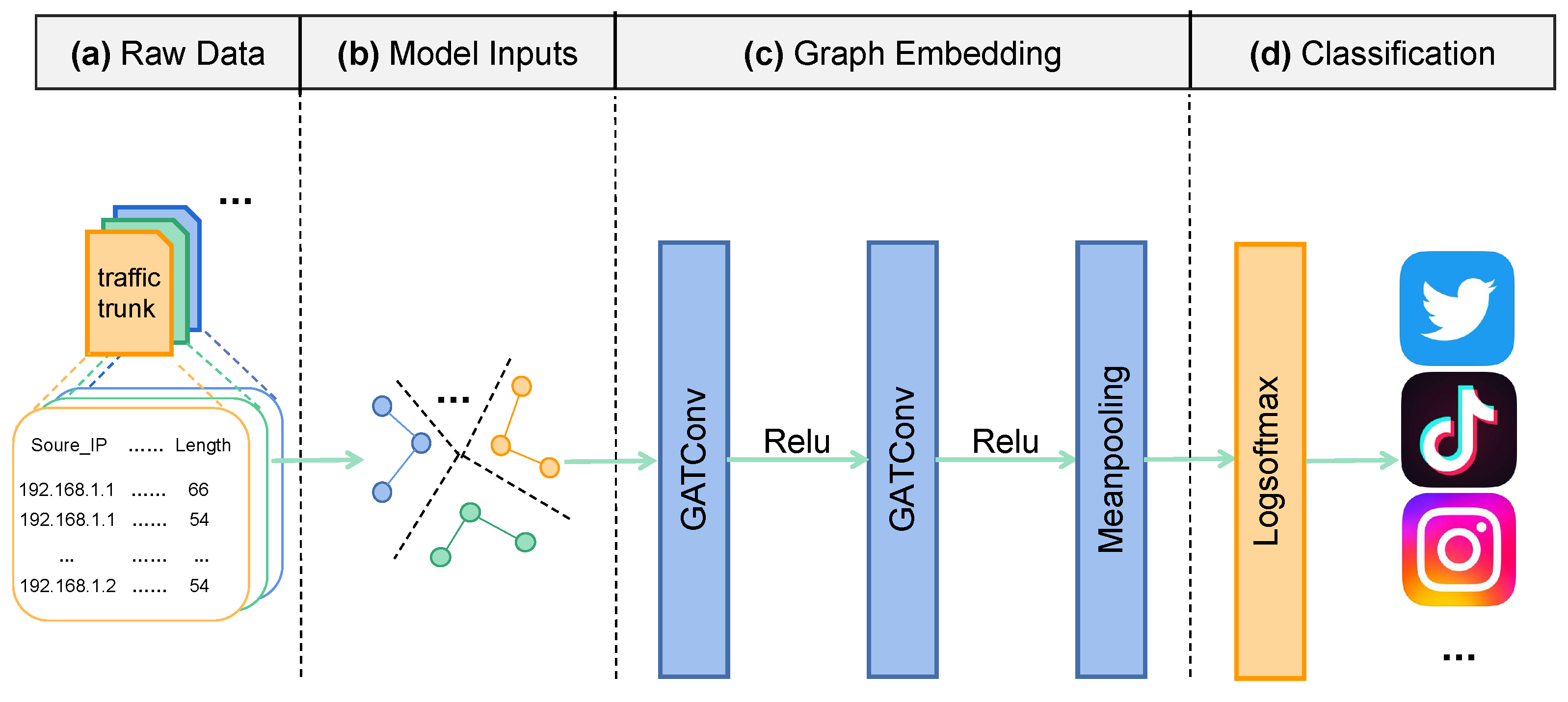
Figure 1 shows the overall architecture of the proposed method: First, the raw traffic is processed into traffic chunks of a fixed time window size; then, the traffic chunks are converted into graphs according to the graph construction method described in Section 3.1. After obtaining the traffic graphs, the designed GNN is used to learn the graph representations. Finally, a Logsoftmax function is used to classify the input traffic chunks. The details of the model composition are introduced in the rest of this subsection.

3.2.1. Problem Statement

Given a set of undirected graphs generated by traffic chunks and their labels, GNNs aim to learn a representation vector that can predict the label of each graph. Let N denote the number of app classes in our dataset. Running the app’s modules results in a large group of packets. With our graph construction method, these packets are represented by a set of graphs $\{g_1,g_2,g_3,\dots ,g_m\}\subseteq G$, where G represents the group of packets and $g\in G$ represents a traffic chunk cut out of the group. The real label of $g_m^i$ is $y_i$, $1\le y_i\le N$. Taking $g_m^i$ as an input, the model predicts according to Equation (1).

$$\widehat{y_i}=\psi (g_m^{(i)};w),\widehat{y_i}\in {\mathbb{R}}^N$$

(1)

where w is the set of model weight parameters, and ${\widehat{y}}_i$ is the probability that the input graph g is predicted as each class (i.e., label). We aim to train $\psi (g_m^{\left(i\right)};w))$ so that the label with the maximum probability in its output is $y_i$.

3.2.2. Raw Data

Since raw traffic is captured over a period of time, we need to slice the traffic into appropriately sized traffic chunks in order to graphically represent the traffic. Therefore, in this stage, sliding window sampling is performed on the original traffic within a defined time window according to the time sequence and fixed time interval, and the collected traffic is saved in the form of multiple corresponding CSV files.

3.2.3. Model Inputs

Employing the graph construction method in Section 3.1, we can convert the collected traffic chunks into graphs. Each flow in the traffic chunk is represented as a node of its graph, standardizing all node features. Flows are connected according to the time correlation (i.e., graph edges between nodes). The converted graph is saved as trainable data according to the structural information and node feature matrix.

3.2.4. Graph Embedding

GATconv. The GAT layer [30] consists of a GCN layer and an attention mechanism. We adopt multi-head attention (i.e., multiple sets of mutually independent attention mechanisms). In the process of aggregating neighbouring information, the GAT layer introduces an adaptive weight matrix for learning. Therefore, the method can avoid introducing too many learning parameters, enabling the efficient representation of graph attention models. The formula for calculating the importance $e_{ij}$ from node j’s features $\overrightarrow{h_j^{\prime }}$ to node i’s features $\overrightarrow{h_i^{\prime }}$ is shown in Equation (2) from [30]:

$$e_{ij}=a(\mathbf{W}\overrightarrow{h_i^{\prime }},\mathbf{W}\overrightarrow{h_j^{\prime }})$$

(2)

where $\mathbf{W}$ is the weighted matrix, and a is a shared attention mechanism for performing self-attention on the nodes. The model chooses not to drop features or attention weight and employs LeakyReLU non-linearity with a negative input slope of $\gamma =0.2$ (i.e., the default setting in [30]). The new $e_{ij}$ is calculated by Equation (3) from [30]:

$$e_{ij}=LeakyReLU({\mathbf{a}}^T[\mathbf{W}{\overrightarrow{h}}_i]\left|\right|\mathbf{W}{\overrightarrow{h}}_j\left]\right)\left)\right])$$

(3)

From the perspective of traffic, the $e_{ij}$ represents the weight of flow j (i.e., a neighbouring flow of flow i) to flow i. Since these neighbouring flows have different importance to flow i, flow i will give different weight to messages delivered by neighbours when performing state updates. For example, flow i is a flow related to the application’s functions, but flow j is a flow generated by a third-party library. Flow j is not important to flow i, so flow i reduces the importance of flow j when performing state updates. To better assign weights, it is necessary to normalize the attention coefficients $e_{ij}$ calculated by all neighbours of node i. The normalization is calculated using Equation (4) from [30]:

$${\alpha }_{ij}=softma{x}_j\left(e_{ij}\right)=\frac{exp\left(e_{ij}\right)}{{\sum }_{k\in {\mathcal{N}}_i}exp\left(e_{ik}\right)}$$

(4)

where $k\in {\mathcal{N}}_i$ is a neighbour from node i. The coefficient calculation of the attention mechanism is fully expanded using Equation (5) from [30]:

$${\alpha }_{i,j}=\frac{exp\left(LeakyReLU\right({\mathbf{a}}^T[\mathbf{W}{\overrightarrow{h}}_i\left|\right|\mathbf{W}{\overrightarrow{h}}_j\left]\right))}{{\sum }_{k\in {\mathcal{N}}_i}exp\left(LeakyReLU\right({\mathbf{a}}^T[\mathbf{W}{\overrightarrow{h}}_i\left|\right|\mathbf{W}{\overrightarrow{h}}_k\left]\right))}$$

(5)

After calculating the coefficient of the attention mechanism, the node’s new feature is calculated using Equation (6):

$$\overrightarrow{h_i^{\prime }}=ReLU\left(\sum _{k\in {\mathcal{N}}_i}{\alpha }_{ij}\mathbf{W}{\overrightarrow{h}}_k\right)$$

(6)

Through the calculation of Equation (6), each flow in the traffic chunk updates its state according to the messages delivered by other neighbouring flows. This takes into account the influence of other flows. To avoid overfitting, it is beneficial to add the ReLU activation function.

To improve the expressiveness and training stability of the model, we extend it with a multi-head attention layer. This is based on the concatenation $\left|\right|$, the calculation for K-independent attention mechanisms is shown in Equation (7):

$$\overrightarrow{h_i^{\prime }}={\left|\right|}_{k=1}^{K}ReLU\left(\sum _{j\in \tilde{N}\left(v_i\right)}{\alpha }_{ij}^{\left(k\right)}{\mathbf{W}}^{\left(k\right)}\overrightarrow{h_j}\right)$$

(7)

Readout layer. Since our classification task concerns graph classification, and focuses on the global information of the graph data, including graph structural information and node attribute information, the proposed model needs to fuse the global information for learning. In CNNs, hierarchical pooling is used to extract global information. In this model, we use mean pooling (i.e., apply average pooling over the nodes in the graph) for efficient extraction of higher-level information, discussed in Section 4.2. This aggregates all nodes after multiple iterations in a single pass through the readout mechanism, similar to a graph-based mean function, and then outputs a global representation of the graph. The formula of the readout mechanism is defined in Equation (8):

$$y=Readout(\{{\overrightarrow{h}}_i^{\left(k\right)}|\forall v_i\in \mathcal{V}\})$$

(8)

where y is the output of the pooling layer, $Readout$ is one of the readout functions, ${\overrightarrow{h}}_i^{\left(k\right)}$ is the feature matrix of node i after k iterations, and $v_i\in \mathcal{V}$ is one node of the set of all nodes.

3.2.5. Classification

After extracting the global features of the graph, we can use this to make predictions about the labels of the input graph. The softmax function is generally used for the output of multi-classification problems. It is an activation function that normalizes a vector of values to a vector of probability distributions, and the sum of the individual probabilities is 1. We choose the Logsoftmax function to apply the $log\left(Softmax\right(x\left)\right)$. The calculation is shown in Equation (9):

$$LogSoftmax\left(x_i\right)=log\left(\frac{exp\left(x_i\right)}{{\sum }_{j}exp\left(x_j\right)}\right)$$

(9)

3.2.6. Loss Function

Mobile app classification is a multi-classification task, so we used the cross-entropy loss function to calculate the loss between the predicted values $\widehat{y}$ and the ground truth y. The calculation is shown in Equation (10):

$$L=-\frac{1}{\left|X\right|}\sum _i^{\left|X\right|}\sum _j^{N}I(y_i=j)log\left({\widehat{y}}_{ij}\right)$$

(10)

where $\left|X\right|$ is the number of model inputs X and $I(y_i=j)=1$ if $y_i$ is j, else 0. We used the Adam optimizer to minimize the loss during training.

4. Experiments and Results

4.1. Preliminary Results

Methods of comparison. To provide a comprehensive view of the performance of the proposed model, we make a comparison with three typical methods. All methods are briefly presented in the following. For a fair comparison, these methods must be tuned to obtain the best accuracy on the evaluation dataset.

• Appscanner: Appscanner is a flow-based method. To perform mobile app classification on a 50 min capture of mobile traffic, the method extracts statistical features of the packet length (e.g., mean, skew) of incoming, outgoing, and complete flows to train machine learning models, including RF and SVM. To make Appscanner perform better on our dataset, we adopted ensemble learning to make improvements to Appscanner, specifically, a hard voting scheme (i.e., selecting the label with the most algorithmic output for a given instant).
• FlowPrint: FlowPrint is a semi-supervised approach for fingerprinting mobile apps from mobile traffic. It creates fingerprints based on 5 min captures of traffic and strong correlations (i.e., cross-correlations). Instead of applying machine learning models to identify which app a fingerprint belongs to, FlowPrint leverages the similarity (i.e., Jaccard similarity [23]) of the fingerprint to be predicted and the known fingerprint clustered into an app in advance to set a predefined similarity threshold.
• MappGraph: MappGraph’s classification component are traffic chunks as previously defined. First, the method extracts traffic features by constructing graphs, building graph nodes with the target IP address and port number as tuples and adding edges via cross-correlation. This is required for node-associated features and edge-associated weights. Then the method uses a GNN model called DGCNN [31] to train and test the dataset, which is described below.

Hardware. All the traffic classification experiments were carried out on a server with Intel core Duo 3.70 GHz with 32 GB memory.

Evaluation criteria. To evaluate the performance of our classification model against others listed, we adopted the following criteria, including precision, recall, F1 measure, and accuracy, where TP refers to the number of true positives, FP refers to the number of false positives, FN refers to the number of false negatives, and TN refers to the number of true negatives.

Precision is calculated according to Equation (11).

$$precision=\frac{TP}{TP+FP}$$

(11)

Recall is calculated according to Equation (12).

$$recall=\frac{TP}{TP+FN}$$

(12)

F1-measure is calculated according to Equation (13).

$$F1=\frac{2\ast precision\ast recall}{precision+recall}$$

(13)

Accuracy is calculated according to Equation (14).

$$accuracy=\frac{TP+TN}{TP+TN+FP+FN}$$

(14)

In simple terms, precision is the percentage of detected traffic that is relevant. Recall measures the proportion of certain apps detected. However, high precision or high recall alone does not fully evaluate the performance of the model. As a harmonic mean, the F1 measure considers both of them. Furthermore, accuracy indicates how many correct classifications were made in the classification results.

4.2. Dataset Construction

Raw dataset and pre-processing: The dataset [32] in MappGraph focuses on Android apps and adopts eight different kinds of smartphones to run mobile apps. Under the controlled traffic collection environment (i.e., a fixed WiFi router), the traffic is generated by popular (i.e., the number of installs) mobile apps from Google Play with student volunteer use. This is more similar to real-world traffic because of human use instead of user simulation scripts. Each app has more than 30 h of traffic stored as PCAP files. After converting all the PCAP files to CSV files, the size of the traffic was more than 50 GB. To obtain graphs from the basic dataset, we sampled raw traffic every 3 min using a sliding window of 5 min, and then used the graph construction method (with a time slice of 10 s) in Section 3.1 to convert the sampled traffic into a graph, where each graph structural and node feature information were saved. In our experiment, the information was saved in the DGL library, a Python library for building GNNs. With our method, the number of graphs generated based on 5 min of traffic was more than 80,000.

Train and test datasets: To ensure that our experiments were comparable, we used data processing hyperparameters in MappGraph [14] to ensure that our underlying dataset was identical to its composition. In more detail, we divided the dataset into a 8:2 ratio, randomly selecting 80% of the graph set generated by each application for training and 20% for testing. The final graphs used for training were more than 60,000, and the test set had more than 17,000 graphs. Moreover, 10-APP, 20-APP, …, 101-APP ten datasets application lists were all obtained from [32]. These lists were consistent with MappGraph’s application lists during the experiment.

4.3. Hyperparameter Tuning

In this subsection, we present the hyperparameters used in the model. We used Pytorch and DGL to implement the deep learning model. To obtain a model with strong generalization capabilities, we needed to adjust the hyperparameters in our model. This is usually a challenging task as we have a larger number of training instances (i.e., 60,000) and many hyperparameters to set. Thus, we adopted NNI (https://github.com/microsoft/nni, accessed on 5 April 2023) (i.e., a tool to find the optimal hyperparameter within the set range) to help us complete the search for hyperparameters, including hidden dimensions and headers in GAT layers, where the setting of the hidden dimension was 50, and the header was set to be 9. Furthermore, other hyperparameters are shown in following.

Learning rate. The size of the learning rate has a lot to do with the training speed of the model. When the learning rate is too large, the model may fail to converge, jumping repeatedly at a certain convergence point; when the learning rate is too small, the model will converge slowly, and the training will be expensive.

Table 2. Impact of different Learning Rate (LR).

LR	1 × 10${}^{-2}$	5 × 10${}^{-2}$	1 × 10${}^{-3}$	5 × 10${}^{-3}$	1 × 10${}^{-4}$	5 × 10${}^{-4}$	1 × 10${}^{-5}$
Accuracy	0.8232	0.0175	0.9739	0.9546	0.9477	0.7085	0.7296

shows the impact of different learning rates on the classification accuracy. According to the table, we set the learning rate to 0.001.

Batch size.

Table 3. Impact of different batch sizes, where CTT is the classifier training time.

Batch Size	10	30	50	70	100	150	200	250
CTT/epoch(s)	112	44	29	23	15	13	12	9
Accuracy	0.9641	0.9489	0.9383	0.9731	0.9739	0.9731	0.9704	0.9732

shows the impact of different batch sizes on the classification accuracy. It can be seen that the training time of the model decreases as the batch size increases. However, the training accuracy only fluctuates by 3% at most. The larger the batch size, the lower the accuracy, but this is slight. According to the table, we set the batch size to 100. It can be seen from the table that values around 100 can also be selected.

Training epochs. The training epochs are closely related to the final classification performance of the model. The more epochs the model is trained on, the better the model fits the input data.

Table 4. Impact of different training epochs.

Epochs	1	2	3	4	5	10	20	30
CTT(s)	34	52	71	90	109	188	346	496
Accuracy	0.8678	0.9206	0.9394	0.9491	0.9493	0.9643	0.9712	0.9739

shows the impact of different training epochs on the classification accuracy. It can be seen that the training time is positively correlated with the classification performance of the model. However, it can also be seen from the table that too much training does not greatly improve the classification accuracy (e.g., only a 0.003 improvement over 10 epochs). Thus, we set the training epochs to 30.

The number of GAT layers. The proposed model is implemented based on the GAT layer. To find out how many layers are optimal, we designed a layer stacking experiment. In general, the deeper the neural network, the better its classification, and the more training time is spent on each epoch. However,

Table 5. Impact of a different number of GAT layers.

Number	1	2	3	4	5	6	7
CTT/epoch(s)	8	15	21	25	28	30	33
Accuracy	0.9618	0.9739	0.9694	0.9658	0.9615	0.9580	0.9558

shows that a two-tiered network structure may be optimal. As a result, the number of GAT layers is set to 2.

Readout layers. As introduced in Section 3.2, the readout layer is significant for learning the global representation of a graph. Sum, mean, and max apply sum, mean, and max pooling over the nodes in a graph, respectively. Top-k [31] first sorts the node features in ascending order along the feature dimension, then selecting the sorted features of top-k nodes (ranked by the largest value of each node). Attention is the global attention pooling from [33]. Since most GNNs are used for node classification and there is no readout layer, we need to select an appropriate readout layer for graph classification.

Table 6. Impact of different readout layers.

Readout Layer	Precision	Recall	F1-Score	Accuracy
Sum	0.9638	0.9626	0.9627	0.9646
Mean	0.9742	0.9739	0.9738	0.9739
Max	0.9730	0.9722	0.9723	0.9722
Top-k	0.9275	0.9224	0.9229	0.9224
Attention	0.9744	0.9739	0.9740	0.9739

shows the impact of different training epochs on the classification accuracy. Although attention and mean have similar effects on model accuracy, the training time spent by attention is higher than the mean, so we use the mean as the readout layer.

4.4. Analysis of the Results

Performance comparison of the mobile app classification methods. In

Table 7. Performance comparison of other mobile application classification methods.

Methods	Precision	Recall	F1-Score	Accuracy
Appscanner	0.8450	0.7646	0.7550	0.7646
FlowPrint	0.8501	0.8234	0.8126	0.8222
MappGraph	0.9329	0.9318	0.9323	0.9318
Our method	0.9742	0.9739	0.9738	0.9739

, we present the performance of the proposed method compared to Appscanner, FlowPrint, and MappGraph. In the table we list the performance of all the techniques in terms of precision, recall, F1-score, and accuracy. The results show that our method outperformed others in all criteria and improved the F1-score by 26% compared to the worst performing classifier. In addition, technologies including MappGraph and our method, adopting graphs and GNNs in mobile traffic interactions and classification, perform better than Appscanner and Flowprint, both based on handcrafted features. Compared to the others, the Appscanner results confirm the fact that consideration of ambiguous traffic is required because ambiguous traffic sharing the same third libraries is very difficult to classify. Furthermore, due to failing to consider graph expression capabilities, FlowPrint, which leverages cross-correlation based on destination IP addresses to deal with ambiguous traffic, only performed slightly better than Appscanner and lower than the others. With a more sophisticated neural network model, MappGraph has the expressiveness of graphs and outperforms Appscanner and FlowPrint with an F1 score of 93%, an improvement of more than 10%. However, its performance is still not as good as our method because we captured the correlations of flows and use attention mechanisms to automatically learn the importance of the different flows in the graph. We design attention experiments in the following. Thus, the reason why our method outperforms the others is because it considers ambiguous traffic, flow correlations, the expressiveness of graphs, and the importance of various flows in a graph.

Comparison with classical DNNs.

Table 8. Performance of our model and other classical deep neural networks.

DNN_models	Precision	Recall	F1-Score	Accuracy
MLP	0.8771	0.8620	0.8694	0.8797
CNN	0.8865	0.8802	0.8833	0.8912
LSTM	0.8389	0.8312	0.8351	0.8392
Our model	0.9742	0.9739	0.9738	0.9739

shows the performance of classical DNNs, including MLP, CNN, and LSTM, widely used in classification tasks [34,35]. They are traditional non-graph algorithms while ours is a graph-based algorithm. From the figure, it can be seen that our model outperforms the DNNs in all metrics because the inter-flow relationships are captured by building graphs, demonstrating the superiority of the classification task translation. LSTM performs worst in them because of the similar packet sequences across different mobile applications. MLP performs better than LSTM but worse than the CNN. This indicates that the classification performance of neural networks correlates with the number of layers.

Ablation experiments on attention. To check the effectiveness of adding attention, which can improve the learning performance of the graph convolution, we performed a relevant comparison experiment. As shown in

Table 9. Ablation results of our model.

Models Based on Ours	Precision	Recall	F1-Score	Accuracy
full	0.9742	0.9739	0.9738	0.9739
1st layer no attention	0.9415	0.9381	0.9387	0.9381
2nd layer no attention	0.9640	0.9631	0.9632	0.9631
all layers no attention	0.8981	0.8938	0.8943	0.8938

, from the perspective of the graph’s learning ability, attention mechanisms work better, where all metrics of the attention model are higher than those of the no-attention models. Removing the first layer’s attention causes a 4% drop in accuracy and removing the second layer’s attention only leads to a 1% drop in accuracy. However, if all attention is removed, the performance of the model drops significantly. This proves that learning the importance of the different flows is very beneficial for improving the classification performance. Because ambiguous flows are a distraction for the app’s classification, paying less attention to them improves the model ability to learn the app’s traffic behaviour.

Training time and computational complexity comparison with MappGraph. As shown in Figure 2, the training speed of our model is extremely fast, converging after 10 epochs. At the same time, its classification performance on the validation set remains high. However, MappGraph consumes a lot of epochs during the training process and cannot reach an acceptable accuracy fast enough. Specifically, the MappGraph model needs to be trained for more than 100 epochs to achieve an accuracy of 0.93, and the model trained for only 10 iterations cannot be used for classification because its accuracy is less than 0.7. In contrast, our model is much faster than MappGraph at obtaining high accuracy, taking only 10 epochs. Moreover, under the same GPU, the training time of the Mappgraph model is a few seconds longer than our model training time per epoch. Therefore, it may not be an appropriate solution for the classification of traffic in real-world scenarios. The reason why MappGraph spends more time on training is that its GNN-based module, consisting of four GNN layers and a global pooling layer, is designed with much more complexity than ours. Each output in its GNN-based module not only passes to the next layer but also to the pooling layer. Conversely, we only designed two layers in the GNN-based module and its transferred value is linear. We also did not add convolutional layers after graph-embedding learning. To detail the amount of computation for both models,

Table 10. Computational complexity of models, where FLOPs are floating point operations.

Models	Layer	Size (MB)	Params	Params %	FLOPs	FLOPs %
Ours	Input	0.5	-	-	118,000	3%
	GAT1	6.9	26,550	10%	1,800,000	47%
	GAT2	7.6	202,500	74%	1,800,000	47%
	Readout	0.3	-	-	90,000	2%
	Dense	0.2	45,450	16%	20,200	0.5%
MappGraph	Input	1.2	-	-	322,560	0.5%
	GCN1	40.3	64,512	1%	10,485,760	18%
	GCN2	44	1,048,576	21%	10,485,760	18%
	GCN3	44	1,048,576	21%	10,485,760	18%
	GCN4	22	524,288	11%	5,242,880	9%
	Readout	70	-	-	18,350,080	31%
	CNN1	8.5	917,760	19%	1,310,720	2%
	MaxPool	2.5	-	-	655,360	1%
	CNN2	3	655,872	13%	131,072	0.2%
	Dense1	4	525,312	11%	524,288	0.9%
	Dense2	0.6	103,525	2%	51,712	0.1%

shows the computational complexity of the two models, including the number of parameters and floating point operations. From the table, it can be seen that the MappGraph model has a larger computational effort and number of parameters compared to ours. Specifically, the total number of parameters of the MappGrpaph model is about twenty times that of our model, and its floating point operations are about fifteen times that of ours. Thus, our model consumes less time and performs better, making is more ideal for real application scenarios.

Different number of application classifications. We evaluated the performance of Appscanner, FlowPrint, MAppGraph, and our method with a varying number of applications by selecting random applications from the original dataset to train and test the model. All the experiments were ran on the same random dataset. As shown in Figure 3, all techniques performed well when the total number of apps was low; however, the performance degrades as the number of apps is increased. It is obvious that the higher the number of apps to be classified, the more difficult it is to classify different apps. This explains why the number of apps in the same category grows with the total number of apps, subsequently leading to more similar traffic being classified. The results indicate that the performance of the other methods, including Appscanner, FlowPrint, and MappGraph, have a dramatic decrease between the smallest and biggest datasets (i.e., 10 apps and 101 apps), while our method maintains high performance in the two scenarios; however, there is inevitably a slight drop of our method in the metrics. Thus, this demonstrates the effectiveness of our method.

5. Discussion

5.1. Reasons for Superiority

In this paper, we showed that the proposed method achieves good performance on a 101 App classification task. Here we discuss why the proposed method performs better than the existing works.

What are ambiguous flows? The concept of ambiguous flows (i.e., flows generated by third-party libraries) was first proposed in [9] and then discussed in [10,11,12,14]. Mobile applications embed third-party libraries to enable features such as advert serving, authentication, etc., but these features are usually not relevant to the services provided by the applications. In addition, flows from the same third-party libraries have small differences. Thus, it is necessary to reduce their impact on accuracy. Appscanner chooses to remove such flows; FlowPrint proposes traffic graphs to create app fingerprints, but uses Jaccard similarity to classify apps; MappGraph was inspired by FlowPrint, and chooses GNNs to solve graph classification problems.

Concurrent multiple flows. When a certain function in an app is activated, multiple flows based on the function are generated concurrently, and most of these flows are related to the function. The number of flows is related to the operating mode of the app, and there is a certain dependence on the flows of the preceding and following periods. For example, opening a short video and scrolling through the comments below the video. Due to the lack of methods that deal with ambiguous flows, Appscanner does not perform as well as ours. Ambiguous flows are highly homogeneous, so they are difficult to associate with different applications. Instead of limiting the classification of flows, the proposed method chooses to use traffic chunks to avoid categorizing ambiguous flows, since the ultimate goal of classifying encrypted traffic is to distinguish the origin of each packet. In this way, the ambiguous flows in a traffic chunk do not fully determine the category of that traffic chunk. FlowPrint and MappGraph perform something similar to our method, but they do not think in terms of flows. FlowPrint takes the destination IP address as a node, and MappGraph takes the destination port and IP address as nodes. In contrast, by building a flow graph based on flow-defined nodes and cross-correlation-defined edges, our proposed method can capture the relationships between flows. This can better describe the mode of operation of an app.

Suitable design for GNN-based models. FlowPrint uses Jaccard similarity (used to find similarities between two collections) to decide which application a fingerprint belongs to. It does not make good use of graph structural information. To extract rich information from graphical data, we designed a GNN-based model. For graphical data, GNNs have been proven to have powerful characterization capabilities, and are widely used in areas such as computer vision, natural language processing, and biology/medicine/chemistry. It automatically learns useful features from the graph data and directly uses them in subsequent classification tasks. MappGraph works similarly to ours, they adopt DGCNN to 101 application classification tasks. However, applications generate concurrent traffic that is not necessarily equally correlated with each other. During state updates of a certain node, when receiving messages from neighbouring nodes, it is not appropriate to treat each message equally. For example, the traffic generated by the advertising service in the application is represented as a neighbouring node, and it is obvious that the messages it delivers are not important for node updates. As a result, we adopted the GAT layer to our model. By stacking layers in which nodes can attend over their neighbourhoods’ features, it implicitly enables specifying different weights to different nodes in a neighbourhood [30]. This means the designed model in the paper can pay more attention to app-specific flows and pay less attention to irrelevant flows.

5.2. The Proposed Method’s Limitations

Although the proposed method achieves a satisfactory performance in the above mobile application classification tasks, it still has some flaws, as follows:

Imbalanced mobile traffic. Mobile traffic collected from the ground truth is often unbalanced. This is because users tend to have a few apps on their phones that are particularly active, while others are launched once every few weeks or months. The same is true of Google Play’s popular app downloads. The public dataset used here only collected a selection of the most popular apps and tried to keep the amount of traffic generated by each app to a small difference. It is only slightly unbalanced, so the proposed model fails to take into account the impact of extremely unbalanced data, which should be explored in future work.

Generalization ability. To date, only one existing public mobility dataset suitable for this work has been found. The generalization ability of the proposed model needs to be tested. This is because performing the classification task on only one dataset is prone to overfitting, although this paper divides the dataset into different sub-datasets. We have added a dropout and training tests on a larger dataset, to avoid overfitting the model. The validity of the proposed method needs to be verified on public datasets that meet the requirements of the proposed method if they become available.

Open world. As with existing techniques, the proposed method treats mobile app classification as a multi-class classification problem in the closed world, where all apps to be identified are already known to the model. However, more generally, there is a massive range of mobile apps in the real world. The model will not know all the apps during training, and thus will only recognize these apps. This is called mobile app classification in the open world, where both unknown and known mobile apps exist. Therefore, it is necessary to classify mobile apps in the open world.

App updates. Apps will be updated from time to time with new iterations, and even small updates every few days, such as TikTok. As a result, mobile traffic generated from apps will constantly evolve with app updates. This leads to the fact that previously created fingerprints will fail to work when classifying existing mobile apps, thus requiring the mobile traffic to be re-collected and the neural network to be re-trained. As the dataset used does not collect traffic after app updates, it is unknown whether our model can accurately identify the updated app after training with the old traffic dataset. In future work, we will explore fingerprint ageing.

Simultaneous running apps. During the collection phase of the dataset, mobile apps are executed one at a time. Therefore, the collected traffic is pure, with no interference from other apps. However, it is quite common for mobile devices to run multiple apps at the same time, such as music streaming and instant messenger apps. This makes mobile traffic extremely complex, and it is already difficult to manually extract from such traffic to obtain an accurate dataset. Therefore, the proposed method can currently only accurately classify single multi-category mobile traffic, but cannot classify composite mobile traffic.

Online mobile app identification. Online analysis of network traffic is essential. Without considering open world and simultaneous running app problems, after training, our model can be deployed in real environments. However, the traffic chunk and graph building are not flow-oriented, which means that constructing application fingerprints needs to be performed offline. To analyse mobile traffic in real-time, a straightforward improvement is to specify the size of the sliding window, collecting traffic samples every few minutes, and perform pre-processing such as cleaning and segmentation of the raw traffic. Large traffic chunks can enrich the behavioural patterns of an application but comes with a high computational overhead. Small traffic chunks, however, cause the opposite. Thus, this requires careful consideration in terms of accuracy, computational overhead, and time cost.

6. Conclusions

In this paper, we proposed an efficient and fast method for mobile app classification. We learnt that ambiguous traffic has a notable impact on mobile traffic classification from existing works. To mitigate such an impact, we developed a new method to process mobile traffic and capture relationships between flows by constructing mobile traffic interaction graphs. The constructed mobile traffic interaction graphs help classify different mobile traffic because of representations of mobile apps’ communication behaviour. We developed a deep learning model to solve the graph classification problem. With an attention mechanism, our model can automatically learn the importance of the different flows generated by mobile apps during communication. We ran numerous experiments in a variety of scenarios and compared the performance of our method to three other methods in the mobile traffic classification landscape (i.e., Appscanner, FlowPrint, and MappGraph). We also set up ablation experiments to show the validity of our proposed graph construction method and deep learning model. The experimental results show that the proposed method outperforms the other methods. It improves for all the criteria (i.e., accuracy, precision, recall, and F1 score) by at least 20% over two of the state-of-the-art methods. It also significantly improves the training speed, half that of MappGaph, and can achieve acceptable accuracy much faster compared to MappGraph. In future work, we plan to make the proposed method more adaptable to traffic changes.