Abstract
Since the number of acquired images and their size have the tendency to increase, their lossy compression is widely applied for their storage, transfer, and dissemination. Simultaneously with providing a relatively large compression ratio, lossy compression produces distortions that are inevitably introduced and have to be controlled. The properties of these distortions depend on several factors such as image properties, the coder used, and a parameter that controls compression, which is different for particular coders. Then, one has to set a parameter that controls compression individually for an image to be compressed to provide image quality appropriate for a given application, and it is often desirable to do this quickly. Iterative procedures are usually not fast enough, and therefore fast and accurate procedures for providing a desired quality are needed. In the paper, such a procedure for two coders based on discrete cosine transform is proposed. This procedure is based on a prediction of mean square errors for a given quantization step using a simple analysis of image complexity (local activity in blocks). The statistical and spatial–spectral characteristics of distortions introduced by DCT-based coders are analyzed, and it is shown that they depend on the quantization step and local content. Generalizing the data for sets of grayscale test images and quantization step values, it is shown that the MSE can be easily predicted. These predictions are accurate enough and can be used to set the quantization step properly, as verified by experiments performed using more than 300 remote sensing and conventional optical images. The proposed approach is applicable to the lossy compression of grayscale images and the component-wise compression of multichannel data.
1. Introduction
A tremendous number of images of different origins are acquired nowadays. Ordinary customers acquire a huge number of color photos and upload them to the Internet [1]. Numerous remote sensing (RS) spaceborne and airborne imagers acquire many images each day [2,3]. Medical diagnostic complexes provide doctors with several types of image data [4], Internet shops and other services use advertising images [5], and so on.
Images acquired by the aforementioned systems have various properties, but there are common tendencies for them. Firstly, their number rapidly grows [6,7]. Secondly, the average size of images increases as well. Color photos become larger due to better digital cameras; a better spatial resolution as well as the use of multichannel imaging mode lead to larger-sized remote sensing images; the size of medical images has the tendency to increase, too. Then, to transfer, store, and disseminate such images, data compression should be used. Lossless compression techniques are mostly unable to ensure a desired compression ratio (CR) [8,9,10]. Moreover, lossy image compression methods are able to produce considerably larger CRs that can be varied using a parameter that controls compression (PCC) [11,12,13,14]. This can be a quality factor (QF) used in JPEG [11], the bits per pixel (BPP) employed in JPEG2000, the quantization step (QS) utilized in DCT-based coders [13], Q-parameter in better portable graphics (BPG) coder [14], etc. A general tendency that is valid for most images is that a larger CR (associated with a smaller QF or BPP or a larger QS or Q) results in greater degradation and worse quality according to any metric, whether conventional or visual [11,12,13,14]. Then, it is necessary to find an appropriate compromise between the introduced distortion (quality of a compressed image) and the CR for a given application and an image to be compressed [2,3,15].
Depending on the application, this compromise (and imposed restrictions) can be different. Some examples are the following:
- Ensure that the CR is as large as possible with the simultaneous provision of acceptable visual quality; in this sense, two tasks have to be solved:
- To find a coder that provides a larger CR for a given image and a given quality;
- To find such a CR that distortions do not exceed the chosen threshold according to a considered quality metric.
- Provide that (diagnostically) valuable information is not lost under the attempt to increase CR for a chosen coder;
- Carry out lossy compression with the simultaneous provision of acceptable quality as quickly as possible or within a certain time interval for a chosen coder and a quality metric threshold.
To solve the aforementioned tasks of reaching an acceptable compromise, one has to answer many questions, including the following:
- What quality metric should one use?
- What are the metric values (thresholds) that correspond to the appropriateness of introduced distortions? With what accuracy should they be provided?
- How should one compare the performance of compression techniques, and what constitutes a good coder nowadays?
- What are the existing procedures for providing the desired quality, and what are their advantages and drawbacks?
A metric to be used should satisfy several requirements. In particular, it has to be adequate for a given application, its properties have to be thoroughly studied, and it should be calculated quickly enough. The mean square error (MSE) is one such metric. Its calculation is very fast, and the MSE properties (in particular, with application to lossy image compression) are well studied. In particular, the Spearman correlation for the MSE and mean opinion score (MOS) for three subsets of images with distortions dealing with lossy compression in the database TID2013 [16] is equal to 0.914, and it is better than the correlation of SSIM [17] and MOS (0.893) but worse than for MOS and some modern visual quality metrics. Thus, the MSE is quite an adequate metric for compressed images. It is also known that if distortions are similar to additive white Gaussian noise, then they are practically invisible for noise variance about 20 and less (for images represented by 8-bit data), i.e., for a peak signal-to-noise ratio (PSNR) of about 35 dB or more [8]. The MSE changes (differences) by 10 …20% can be very hardly noticed in compressed images by visual inspection. Hence, in fact, the first two questions have been answered.
The performance of image compression techniques is usually analyzed by exploiting rate/distortion curves, i.e., dependencies of a parameter that characterizes image quality on PCC or CR. To obtain correct conclusions, such an analysis has to be performed for many images and for a wide range of CR (PCC, image quality). The results of performance analysis carried out for several compression techniques [8,9,13] show that lossy compression techniques based on orthogonal transforms including DCT [10,11,14] provide good results. Some DCT-based coders sufficiently outperform the JPEG and JPEG2000 [12] standards. Since they are based on DCT, they can be easily incorporated into existing software- and hardware-image-processing tools, including on-board systems and devices of remote sensing image compression [18]. Because of this, the analysis below is concentrated on the prediction of the MSE for the coders AGU [19] and ADCT (advanced DCT) [20], assuming that the proposed approach can be useful for other DCT-based compression techniques.
The paper structure is as follows. In Section 2, related work is discussed, whereas Section 3 briefly describes the considered compression techniques and analyzes the existing solutions for MSE prediction. Statistical and spatial correlation analysis of distortions introduced by lossy compression is carried out in Section 4. Dependencies of statistical characteristics of distortions on image local activity are studied in this Section as well. A method for MSE prediction and its accuracy analysis are presented in Section 5. Finally, the conclusions follow in Section 6.
2. Related Work
The problem of providing desired values of the MSE (as well as other metrics) has been considered earlier in several papers [13,21,22,23,24,25,26]. The three main approaches are as follows.
Firstly, an iterative procedure presuming multiple image compressions/decompressions with quality metric (e.g., the MSE) estimation and PCC refining at each iteration can be used [13]. The advantage of such a procedure is that it is able to ensure high accuracy when providing a desired value of a considered metric [13], e.g., the PSNR with an accuracy of less than 0.2 dB (the MSE with a relative error less than 6%). The drawback is that the number of iterations is unknown in advance and, because of this, the requirements imposed on the maximal time of compression can be sometimes not satisfied. In addition, the approach requires more computations than the other two methods, and, thus, it is not attractive from the viewpoint of green technologies [27].
Secondly, the so-called two-step procedures have been developed recently [23,28]. They are based on obtaining an average rate-distortion curve for a given coder (for example, the MSE or PSNR on the QS) in advance (off-line). This curve is then used to determine a starting point (the initial QS) for image compression, decompression, and metric calculation. Then, using the average curve derivative, the final QS is calculated, and the final compression is carried out. This approach is, on the average, considerably faster than iterative. However, its accuracy is worse than the iterative approach and, in some situations such as quite a large CR, can be inappropriate for practice. Moreover, two compression steps and one decompression are needed in any case. This can be acceptable if both compression and decompression are fast enough but can make problems if either compression or decompression are too slow.
Thirdly, several approaches that can be treated as prediction-based have been put forward [22,24,25,26,29]. Their main advantage is that they determine the PCC (QS) based on the prediction of metric value. Due to this, no preliminary compression and decompression as for the two-step approach are needed. This allows one to determine the PCC quite quickly. In addition, for the approach [29], the spatial distribution of distortions introduced by lossy compression can be predicted, which can be useful for achieving several goals of further image processing. However, its prediction accuracy is usually worse than for iterative and two-step approaches, and its careful analysis has not been carried out.
Therefore, the goal of this paper is to further advance the approach proposed in our paper [29]. The novelty of this paper consists in two items. Firstly, the spatial distributions of introduced distortions are analyzed. Secondly, the statistical analysis of the MSE predictions for numerous test grayscale images is carried out, including those images not used in obtaining the prediction curves.
3. Description of the Used Coders, Test Images, and Preliminary Analysis of Compression Characteristics
3.1. Used Coders and Test Images
The most known and widely used DCT-based coder is JPEG [30]. Its positive and negative features are well known. In particular, the main drawbacks are the blocking effect and the use of fixed size blocks that limit potential of compression. These drawbacks stimulated studies intent on the fuller exploitation of DCT potential in image and video compression applications. One of extensions is the AGU coder [19] based on the 2D DCT in pixel blocks. In addition, AGU employs an efficient bit plain coding of the DCT coefficients after uniform quantization and decompressed image deblocking. Due to the aforementioned modifications, the AGU coder outperforms JPEG [30], SPIHT [31], JPEG2000 [12], and many other compression techniques [13].
Another compression technique considered in our study is the ADCT coder (ADCTC) [20]. It attempts to avoid the drawback of using fixed block size (inherent for JPEG and AGU) by exploiting partition scheme optimization to adapt the block size to image content. An example is presented in Figure 1, where partition schemes are demonstrated for two QS values for one of the test images. The blocks have a square or rectangular shape, where the side sizes are powers of 2, to provide an opportunity to use fast algorithms of the DCT. The block sizes are larger for more homogeneous regions of images. The partition scheme is not the same for a given image; it changes, with the QS becoming slightly simpler if the QS and CR increase.
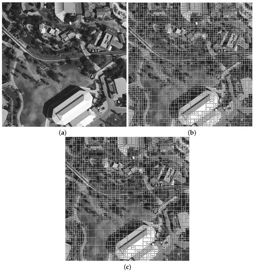
Figure 1.
Illustration of the partition schemes: (a) test image Fr01, and partition schemes for (b) QS = 5 and (c) QS = 20.
The ADCTC requires more computations compared to JPEG and AGU, especially at the compression stage when the partition scheme has to be optimized. Decompression is faster than compression.
At the preliminary stage of our studies, in addition to the test image in Figure 1a, the three other test images given in Figure 2 have also been employed. These are typical remote sensing images of natural scenes of medium complexity.
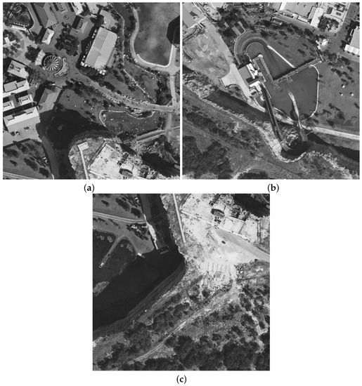
Figure 2.
Testimages used in experiments: Fr02 (a), Fr03 (b), and Fr04 (c).
All of the images are of the size pixels, allowing for the use of coders’ versions freely available at https://ponomarenko.info/agu.htm (accessed on 28 April 2023) and https://ponomarenko.info/adct.htm (accessed on 28 April 2023). Note that an interested reader can find some performance comparison results there.
3.2. Preliminary Analysis of Some Rate/Distortion Characteristics
Recall that our analysis is mainly focused on practical situations when compression is visually lossless or, at least, the introduced distortions are not annoying. This happens if the PSNR is about 35 dB (let us say, from 30 to 45 dB) [32]. As said above, the PSNR is not the best metric if the goal is to adequately characterize the visual quality of compressed images. Hence, the visual quality metric PSNR-HVS-M [33] should be considered as well. It takes into account two important peculiarities of the human vision system (HVS), and its properties have been thoroughly studied in [32]. Similarly to the PSNR, the PSNR-HVS-M is expressed in dB. The properties of the PSNR-HVS-M are important for our further analysis are as follows. The values of the PSNR-HVS-M are larger than the values of the corresponding PSNR if the distortions’ properties are similar to the properties of additive white Gaussian noise (AWGN) and a considered image is able to mask noise (distortions), at least partially (this happens if a distorted image has texture fragments containing many fine details). One more important property is that distortions are visible if the PSNR-HVS-M does not exceed 41 dB [32].
Let us start our analysis from the coder AGU and consider the following three values of the QS equal to 5, 10, and 20. Table 1 contains the following parameters: bpp (bits per pixel) that can be recalculated from the CR as bpp = 8/CR (for grayscale images represented as 2D 8-bit data arrays), the PSNR, and the PSNR-HVS-M.

Table 1.
Characteristics of test image compression for AGU.
As can be seen, the case of QS = 5 can be associated with near lossy compression since for all four test images, the bpp values are slightly larger than 3, the PSNR values are sufficiently larger than 35 dB, and the PSNR-HVS-M values exceed 55 dB. The case of QS = 20 relates to visible distortions that are not annoying distortions. For QS = 20, bpp is about 1.4, i.e., the CR exceeds 5. Since the PSNR values are slightly smaller than 35 dB and the PSNR-HVS-M values are approximately 39.7 dB for all four test images, distortions can be noticed by visual inspection. The case of QS = 10 can be treated as intermediate: the CR is approximately 3.5; the PSNR is approximately 39.7 dB; and the PSNR-HVS-M is approximately 47.3 dB, i.e., distortions are not visible. The presented examples are in good agreement with the results in our paper [13], where it is shown that, on the average, QS has to be set equal to 16 to provide the invisibility of introduced distortions for both considered coders.
From data in Table 1, it might seem that the values of the PSNR, PSNR-HVS-M, and bpp (CR) for a given QS are almost the same, and it is not a problem to provide a desired quality.
However, it is not true (the reason of approximate coincidence of performance characteristics for the considered four test images is that their complexity is similar). In reference [13], it is shown that, e.g., for bpp = 1.6, the PSNR-HVS-M values vary in the limits from 30 dB to 53 dB. It is also shown in [23] that the PSNR values for the same QS can differ by up to 10 dB (for a QS of about 20).
Let us now briefly consider preliminary data for ADCTC. They are presented in Table 2, where the values of the CR/bpp and MSE/PSNR for four test images and three values of the QS are given. As it may be seen, the main tendencies are the same:
Table 2.
Characteristics ot test image compression for ADCTC.
- The CR increases (the bpp are reduced) if the QS increases;
- The MSE increases (the PSNR is reduced) if the QS becomes larger;
- The MSE increases almost proportionally to the QS2; hence, the obtained value for the QS = 5 is
Meanwhile, for QS = 10, the MSE is about 7.5 and is already noticeably less than (8.33), and for QS = 20 this difference further increases (as 400/12 ≈ 33.33). Moreover, the true MSE becomes quite different for the considered test images. A quite thorough analysis of the observed tendencies and the reasons for them has been carried out in [24]. Further, some interesting dependencies from this paper are presented, considering two noise-free images and one noisy image. The noise-free images are “Frisco” and “Airfield”, presented in Figure 3a,b, respectively. As one can see, the image “Frisco” contains many quasi-homogeneous regions, and, thus, it can be treated as simple structure one. Moreover, “Airfield” is approximately of the same complexity as the test images in Figure 2. The third considered image is the same test image “Frisco_std5” but with the artificially generated additive white Gaussian noise (AWGN) with zero mean and noise variance equal to 25. The purpose for considering such an image was to analyze the noise influence on compression characteristics.
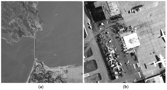
Figure 3.
Noise-free test images “Frisco” (a) and “Airfield” (b).
The dependencies of the MSE determined between the compressed image and the corresponding image before compression for the ADCTC are presented in Figure 4. Although for all three test images the MSE increases if the QS becomes larger, there are sufficient differences. Firstly, the MSE for the noise-free image “Frisco” is always the smallest and, for the QS starting from 10, it is smaller that for two other test images by several times. For QS = 20, the MSE for the noise-free test image is smaller than by about 5 times, i.e., by about 7 dB. Secondly, till QS = 17, the curves for the test images noisy “Frisco_std5” and noise-free “Airfield” practically coincide and the approximate expression (1) is practically valid. However, for a larger QS, the curves behave in a different manner. Thirdly, depending on noise variance, the dependencies are considerably different even for images of the same content (“Frisco” and noisy “Frisco_std5”). This example shows that noise sufficiently influences coder performance.
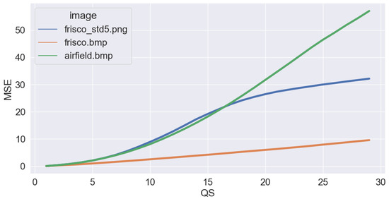
Figure 4.
Dependencies of MSE on QS for ADCTC determined for three test images.
The latter conclusion is also confirmed by the plots in Figure 5 that show the dependencies of the CR on the QS for ADCTC for the considered three images. The CR for the simple structure noise-free image “Frisco” is sufficiently larger than for the test image “Airfield” and noisy image “Frisco_std5”. Only for quite a large QS (i.e., QS = 25) do the CR values for compressed noise-free and noisy images (“Frisco” and “Frisco_std5”) become close, and this happens due to a noise-filtering effect observed for the lossy compression of noisy images.
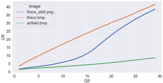
Figure 5.
Dependencies of CR on QS for ADCTC determined for three test images.
Differences in the dependencies in Figure 4 and Figure 5 are explained in [24] in detail, where it is shown that the distributions of DCT coefficients differ significantly for the considered three images and parameters of these distributions (e.g., the percentage of DCT coefficients that become zero after quantization), which are in a rather strict connection with the MSE and CR. Meanwhile, the main goal of the analysis above was to demonstrate variability of the MSE for the same QS and coder depending on the image complexity and the presence of noise. At the same time, the presented results can be treated as the background of the idea that the MSE can be predicted for a given QS if an image to be compressed is somehow quickly analyzed to determine its main properties. Thus, let us briefly recall the existing approaches and solutions.
The paper [21] was probably the first interesting attempt to predict the MSE and PSNR for the JPEG coder. The authors have assumed that the distribution of AC DCT coefficients in pixel blocks is close to Laplacian. Thus, by estimating the distribution scale S and using the a priori obtained dependence of the MSE on , it is possible to predict the MSE. However, there are two drawbacks of this approach. Firstly, the authors of [21] have proposed to perform scale estimation for AC DCT coefficients calculated in all blocks of an image planned to be compressed. This means that the first stage (obtaining DCT coefficients) in pixel blocks takes the same time and the first stage of compression itself. Thus, prediction is not faster than compression or time expenses are of the same order. The second drawback is that the distribution of AC DCT coefficients can differ from Laplacian. This leads to prediction errors that might exceed 1 dB.
If one deals with the AGU and ADCT coders, the prediction should be considerably faster than the compression. Based on the results in [21], two ways to better predict the MSE for advanced DCT-based coders [22,24,25,26] have been put forward. The main ideas in the papers [25,26] are two-fold. Firstly, it is possible to predict the MSE by processing original and quantized DCT coefficients in pixel blocks with recalculating (correcting) the predictions for the AGU and ADCT coders. Secondly, it is not necessary to consider all of the possible block positions—it is enough to analyze 500–1000 randomly chosen blocks. The predictions are quite accurate, but the DCT still needs to be carried out for many blocks.
Another approach [22,24] is based on using the following expression:
where is a function of one or several parameters that describe the properties of an image to be compressed (its complexity or simplicity, the presence and amount of noise, etc.). In the simplest case, X is the aforementioned percentage of AC DCT coefficients that become zero after quantization. The drawbacks of this approach are two-fold. Firstly, it is needed to estimate the statistics of the DCT coefficients, i.e., to apply 2D DCT in blocks and comparison operations taking more time than just DCT. Secondly, the method’s accuracy is not high if the percentage exceeds 0.8, i.e., for quite large QS (e.g., QS = 20).
Therefore, it is desirable to develop a technique that provides accurate prediction without applying DCT (and faster than existing techniques). It is also desired to utilize an accurate and universal method where universality is considered appropriate for a wide set of images and QS values.
4. Detailed Analysis of Distortion Properties
The necessity to study the statistical and spatial–spectral properties of distortions introduced by different coders is significant for several reasons. Firstly, it has been stated in [34] that the distortions due to lossy compression have to be of limited intensity and have spatially “uniform” distribution to avoid artifacts (including classification artifacts). Secondly, the results in [26] have demonstrated that the distortions have a distribution close to Gaussian for relatively small CR and QS for complex-structure images, whereas the distribution might be non-Gaussian for simple-structure images. However, the reasons for this have not been explained. Because of this, it is worth recalling the data recently presented in our paper [29], where the visual and quantitative analysis of difference images has been performed. Note that difference images are quite often used in analysis of image lossy compression and denoising. Let be an original image having the size of pixels and represent the corresponding compressed image. In simulations, both images are available, and the difference image can be calculated as
In most practical situations, are integers that can be negative, positive, and equal to zero.
For visual inspection, there are several ways to present difference images, e.g.,
- As absolute values of differences (including preliminary magnification);
- Using a pedestal, for example, as
One example of has been determined for the test image Fr01 compressed by AGU with QS = 20. The fluctuations (distortions) can be hardly noticed in the compressed image since PSNR is about the distortion visibility threshold (slightly smaller than 35 dB). Therefore, the 3D plot of the absolute values of differences is presented in Figure 6 instead of the difference image for better visualization. The visualized distortions are absolutely not seen for QS = 5 and QS = 10. Because of this, the difference images are not shown here.
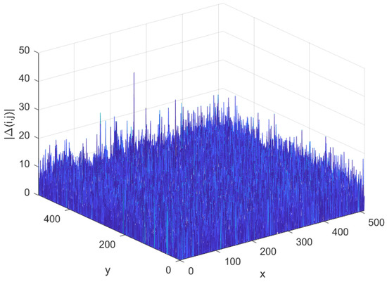
Figure 6.
The 3D plot of the absolute values of difference image for the compressed image Fr01 for QS = 20.
Since it is expected that differences (3) can be a non-stationary 2D process, its spatial spectral or correlation analysis should be performed with care. One methodology of such an analysis applicable for signal-dependent or spatially invariant data has been proposed in [35,36]. One has to determine the mode of local kurtosis estimates obtained in the DCT domain. If this mode is smaller than 3.75, the noise can be assumed to be spatially uncorrelated.
The obtained results are presented in Table 3. As one can see, the distortions can be considered spatially uncorrelated for all four test images and all three QS values. However, one can observe a tendency for the mode to increase (i.e., to a larger spatial correlation of distortions) when QS increases.
Table 3.
Mode of local kurtosis estimates.
A similar analysis has been carried out for the ADCT coder. The results are practically the same—the distortions can be considered spatially uncorrelated, at least, for QS ≤ 20.
Let us carry out statistical analysis in blocks keeping in mind the possible non-stationarity of distortions. Let us employ non-overlapping pixel blocks and calculate in each of them the following two parameters (where each block position is defined by the left upper corner coordinates n and m:
where and .
It is possible to present the obtained data as scatter-plots of root mean square error (RMSE) of distortions vs.RMSE of characterizing noise local (content) activity. For the test image Fr01, the obtained scatter plots are given in Figure 7 for three values of QS. Their analysis shows the following:
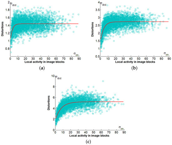
Figure 7.
Scatter plots vs. for the test image Fr01 for QS equal to 5 (a), 10 (b), and and 20 (c).
- One can observe large areas of where are, in general, random, but their mean is practically constant; later, such areas will be called saturation areas;
- If is quite small, there is a tendency of to decrease (on average), with a reduction in ; this tendency may be observed when .
The scatter plots obtained for the other three test images are very similar to those represented in Figure 7. To illustrate this, the scatter plots for the test image Fr02 are given in Figure 8. As it may be seen, the conclusions that can be drawn from their analysis are the same as given above.
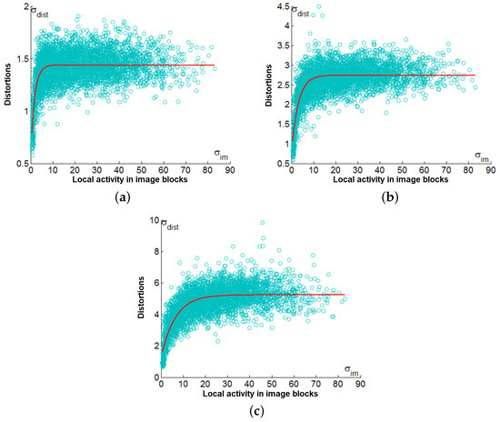
Figure 8.
Scatter plots vs. for the test image Fr02 for QS equal to 5 (a), 10 (b), and and 20 (c).
Having obtained such scatter plots, it is possible to carry out regression, i.e., to fit the curves. For this purpose, the following approximation is used:
where a, b, and c are the function parameters to be estimated. For curve fitting and the estimation of its parameters, the MATLAB fminsearch function may be used, which allows one to find a minimum of unconstrained multi-variable function using the derivative-free method.
The parameters of the fitted curves are given in Table 4. For the same QS, the parameter values of the fitted curves for the considered test images are very similar. This especially relates to the parameter c that describes the “saturation level”.
Table 4.
Parameters of the fitted curves (AGU).
The presented scatter plots explain why the MSE of distortions introduced by lossy compression into simple-structure images differs from the MSE of introduced distortions for complex-structure images. Complex-structure images mostly have blocks where is large enough due to high local activity, and then for such blocks is, on average, approximately equal to . Then, the MSE for the entire image is close to as well. Meanwhile, when QS increases, there are fewer blocks in the saturation area, and the MSE for the entire image is smaller than .
Let us now present the scatter plots of vs. for the ADCT coder. They are given in Figure 9. It is possible to compare the scatter plots in Figure 9 to the corresponding scatter plots in Figure 7 and Figure 8.
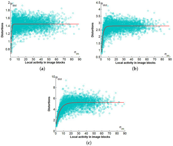
Figure 9.
Scatter plots vs. for QS equal to 5 (a), 10 (b), and 20 (c) for the test image Fr01 (ADCTC).
The comparison shows that the main properties of the scatter-plots are very similar. Again, there are saturation zones observed for where are approximately equal to . When , then decreases, with a reduction in QS.
This reduction can be explained as follows. In quasi-homogeneous image regions (blocks), there is a large percentage of DCT coefficients that are smaller than the QS (especially if the QS is large enough). Quantization errors for such DCT coefficients, on average, have smaller absolute values than the case when most DCT coefficients have absolute values larger than the QS (see the distributions of quantization errors in [21]). Since the quantization errors in the DCT domain are smaller, the local MSEs for the corresponding blocks of compressed images are smaller as well.
The map of in blocks (magnified by 5 for better visualization) for the test image “Frisco” (Figure 3a) is presented in Figure 10a, whereas Figure 10b shows the map of in blocks (magnified by 28 for better visualization) for the same test image. It is clearly seen that is smaller (pixels are darker) in homogeneous regions of the image where the values of are smaller (the pixels are darker).
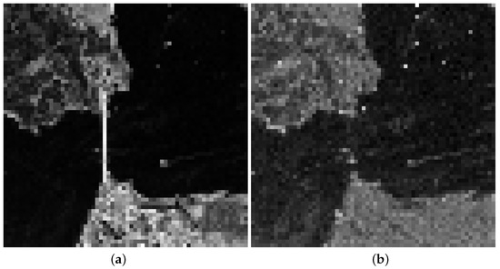
Figure 10.
Maps of (a) and (b) in blocks for the test image “Frisco”.
The scatter plots for other test images are very similar. The parameters of the fitted curves obtained using the approximation (6) are presented in Table 5. In comparison to the corresponding values in Table 4, they are very similar. The only difference is that the values of the parameter c for the ADCT coder are slightly larger. However, they are again approximately equal to QS/3.47 (1.44, 2.88, and 5.76 for QS equal to 5, 10, and 20, respectively).
Table 5.
Parameters of the fitted curves (ADCTC).
Since a great number of and , corresponding to each other, are obtained for three values of QS, it is possible to obtain aggregate scatter plots for both considered coders. Furthermore, the scatter plots in a normalized way as the dependence of vs. are presented. For the coder AGU, the aggregated scatter plot is presented in Figure 11. The general properties of this scatter plot are similar to those presented earlier. There is a monotonously increasing part of the fitted curve observed for and the “saturation part” where is close to unity that takes the place for . The fitted curve is expressed as
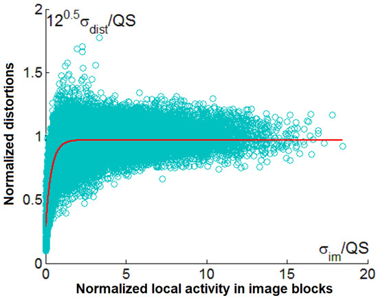
Figure 11.
Aggregated scatter plot for different test images, and QS values for the coder AGU.
Note that the value of the parameter c is not equal to 1, but it is quite close to unity.
Similarly, the aggregated scatter plot has been obtained for the ADCT coder. It is presented in Figure 12. A comparison of the scatter plots in Figure 11 and Figure 12 shows that their main properties are quite close. Note that large ratios relate to “very active” local areas (where sharp edges or large contrast small-sized objects are observed) and quite small QS values.
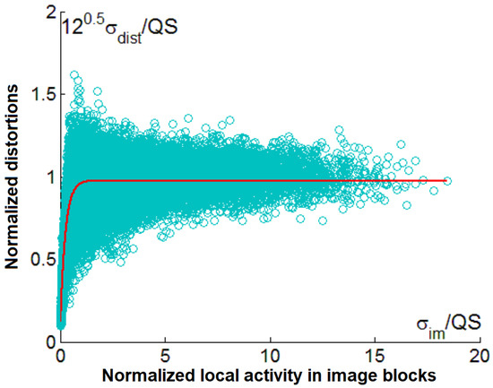
Figure 12.
Aggregated scatter plot for different test images, and QS values for the ADCT coder.
The largest variations of with respect to the fitted curves take place for . Such situations are observed for blocks that correspond to low-contrast edges, details, and textures that are the most typical for natural scene images.
The obtained fitted curve is given as
In this case, the value of the parameter c is even closer to unity.
5. MSE Prediction and Its Accuracy
Having obtained the expressions (7) and (8) for the AGU and ADCT coders, respectively, it is possible to predict for each k-th pixels block of a given image using the corresponding estimate obtained for this block.
For a given block and QS, one has
Assuming the knowledge of the estimates where K denotes the total number of blocks (the questions how the blocks can be positioned and what should be their number will be discussed later), the MSE for entire image can be predicted as
or
where is the value of RMSE in a k-th block determined by the Formula (5). Note that it is very easy to calculate all in advance if the block positions are known in advance as well.
Let us now analyze the accuracy of predicting the MSE for introduced distortions. Table 6 presents the data for the four test images used in forming the scatter plots for the AGU coder. As it may be seen, the true values of the MSE are close to the corresponding predicted ones (); the relative difference is considered small in practical applications as it does not exceed 10%. The data for the ADCT coder for the same four images are presented in Table 7. Their analysis shows that the true and predicted values are also quite close. The maximal difference does not exceed 8%, i.e., 0.3 dB with regard to PSNR.
Table 6.
Comparison of true and predicted MSE values for the AGU coder.
Table 7.
Comparison of true and predicted MSE values for the ADCT coder.
However, the results for images that have not been used in training (obtaining the fitting curves for the scatter plots) are more interesting. Such verification data have been obtained for 16 other test images of different origins. There are some traditional images such as “Lena”, “Baboon”, “Barbara”, “Boat”, “Goldhill”, “Peppers”, and “Man”. There are also highly textural images as “Grass” and “Bikes” (see small copies in Figure 13). Several remote sensing images, such as “Frisco”, “Airfield” (both shown in Figure 3), “Lu01”, “San Diego1”, “a13sm”, “Sent01”, and “Sent02” (see small copies in Figure 13), have also been used. The goal of using images of different origins is to demonstrate that the proposed approach to prediction is applicable in different practical situations.
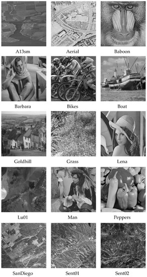
Figure 13.
Small copies of test images used in experiments.
Selected results are presented in Table 8 and Table 9, where the most interesting examples are shown. Alongside with this, statistical results characterizing the accuracy of prediction are presented below.
Table 8.
Comparison of true and predicted MSE values for the AGU coder for sample images used during the experimental verification.
Table 9.
Comparison of true and predicted MSE values for the ADCT coder for sample images used during the experimental verification.
An analysis of data in Table 8 demonstrates the following. Firstly, for QS = 5, the MSE values do not differ significantly (they vary from 1.55 to 2.14), and they are predicted well. Secondly, for QS = 10, the difference in the MSE values increases (they vary from 4.2 for simple-structure image “Lu01” to 7.81 for the complex-structure image “Grass”), but the prediction is still considered accurate enough. Finally, for QS = 20, the MSE may differ noticeably depending on the image complexity (from 10.21 for “Lu091” to 30.92 for the test image “Grass”). However, the predicted values are in good agreement with the true MSE, and this happens for all of the images used in our analysis.
Bias and variance have been also determined for the true and predicted values for all twenty images used in analysis. For QS = 5, they are equal to −0.11 and 0.18; for QS = 10, they are equal to 0.07 and 0.51; and for QS = 20, they are equal to 2.77 and 8.66, respectively. The bias and RMSE constitute less than 15% of the mean values for each QS, and such a level of accuracy is acceptable in practice (in fact, the PSNR is predicted with a maximal error of less than 1.5 dB).
An analysis of data presented in Table 9 shows the following. Firstly, if the QS = 5, the MSE values vary in rather narrow limits (from 1.69 to 2.14), and they can be predicted well enough. Secondly, when the QS = 10, the MSE values vary from 4.61 for the image “Lu01” having simple structure to 8.21 for the image “Grass” with the complex structure. The prediction accuracy is high for all of the images. Thirdly, when the QS = 20, the MSE can vary in wide range, e.g., from 11.25 for the image “Lu091” to 31.92 for the image “Grass”. The predicted values are quite close to the corresponding true ones, and, in fact, this takes place for all of the images employed in our study.
Concerning bias and variance, they are as follows: for QS = 5, they are equal to −0.15 and 0.019; for QS = 10, they are equal to 0.07 and 0.51; and for QS = 20, they are equal to to 2.77 and 8.66, respectively. The bias and RMSE constitute less than 16% of the mean values for each QS, and such a level of accuracy is acceptable in practice (in fact, the PSNR is predicted with maximal error less than 1.4 dB). A comparison of data in Table 8 and Table 9 shows that the values of MSEpred for the ADCT coder are usually slightly larger than for the coder AGU. This conclusion can also be drawn from a comparison of expressions (7) and (8), where the value of the parameter c is larger in the latter case.
Furthermore, the prediction accuracy for the method [22] using the ADCT coder for QS = 20 has also been analyzed. The minimal predicted MSE is observed for the image “Lu01” (11.63), and the maximal (34.43) id observed for the test image “Grass”. The statistical analysis shows that the bias between the predicted and true values of the MSE is equal to −1.44, and the variance equals 7.11. This means that the prediction accuracy is of the same level as for the method proposed in this paper.
There are several aspects left for discussion. Firstly, all of the results presented above have been obtained for non-overlapping blocks fully covering the image area. Thus, for the pixels images used in our analysis, the calculation of has been employed. It is possible to expect that the use of overlapping blocks can improve the prediction. Thus, the fully overlapping blocks with their total number equal to 255,025 have been additionally used. However, this has not led to an improvement of the prediction accuracy. Moreover, the values of MSEpred corresponding to each other for the non-overlapping and fully overlapping blocks differ insignificantly—by less than 0.04%. For example, for the test image “Fr04” and Q = 20 (the AGU coder), the values of MSEpred are equal to 22.240 and 22.264 for non-overlapping and fully overlapping blocks, respectively. Furthermore, the case in which 1000 blocks have been placed randomly has been studied. The obtained prediction results practically do not differ from the corresponding data for non-overlapping blocks. Hence, there are some interesting options for accelerating the prediction by analyzing a limited number of blocks.
Starting from the developed method for predicting MSE, in practice one needs an algorithm for providing a desired value of MSEdes. Then, several options can be proposed. For example, in the first step, calculate the correcting factor as
and
then determine
If is quite close to (e.g., if they differ by no more than 10%), the value may be used for final compression. If this condition is not satisfied, the final QS may be calculated as
and applied for compression.
The simplified flowchart of the proposed method is presented in Figure 14.
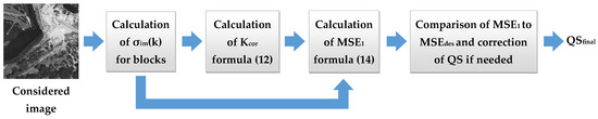
Figure 14.
Thesimplified flowchart of the proposed method.
This algorithm has been first tested for the coder AGU for MSEdes = 20 for all twenty images used in previous studies. The provided MSE varies from 11.87 (image “Barbara”) to 20.59 (image “Grass”), and its bias and variance are equal to 3.22 and 5.79, respectively; hence, this accuracy can be considered satisfactory. The final QS varies from 16.04 for the image “Grass” to 24.99 for the image “Frisco”, i.e., as expected, the final QS is the largest for simple-structure images and the smallest for complex-structure images. As one can see, the provided MSE is, on average, smaller than desired, and this mainly happens for simple-structure images. On one hand, this can be useful in practice since one has some “reserve” in quality just for images for which the distortions are more visible. On the other hand, it is possible to introduce some additional correction to remove the bias.
The proposed algorithm has been also tested for the ADCT coder for MSEdes = 20. The provided MSE varies in its limits from 12.06 for the image “Barbara” to 21.16 for the image “San Diego”. The bias and variance are equal to 2.86 and 6.46, respectively. So, again a bias and an RMSE of errors smaller than 15% have been obtained; such accuracy can be considered satisfactory. The final QS varies in its limits from 16.04 for the image “Grass” to 24.90 for the image “Frisco”.
The additional verification of the proposed algorithm has been made for 300 grayscale versions of pixels images from the TAMPERE17 noise-free image database [37]. The obtained results for MSEdes = 20 are presented in the form of histograms for AGU and ADCT coders in Figure 15. In most cases, the provided MSE values are quite close to MSEdes = 20. Although the provided MSE values are shifted with respect to the desired MSE, and the variance of the final MSE is quite large, an important advantage is that the provided MSE values are mostly smaller than the desired MSE. The smallest provided MSE are observed for images with a simple and specific structure, e.g., those presented in Figure 16. This phenomenon and its reasons are planned to be investigated in future research.
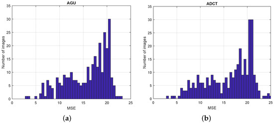
Figure 15.
Histograms of the provided MSE values obtained for 300 images from TAMPERE17 dataset: (a) using AGU coder, (b) using ADCT coder.
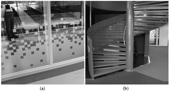
Figure 16.
Two sample grayscale images from TAMPERE17 dataset with the smallest provided MSE values: (a) image no. 257, (b) image no. 263.
As can be seen, the algorithm of the determination of the final QS is computationally very simple. It requires the calculation of twice, where the functions are quite simple; the calculation of ; and elementary comparison and arithmetic operations. Being realized at Intel Core i7 L620 2.00 GHz with 8GB of RAM, it takes 0.363 ± 0.025 s for non-overlapping blocks for an image of size pixels. Recall here that compression by AGU takes 1.020 ± 0.040 s (whilst decompression requires 1.735 ± 0.083 s). Thus, prediction is sufficiently faster than compression. Note that, additionally, it is possible to use a smaller number of analyzed blocks—if, e.g., 1000 blocks placed randomly are used instead of 4096 non-overlapping blocks, predicted MSEs differ by less than 1%; hence, such an approach is appropriate for practice. In this case, prediction can be realized by one order of magnitude less time than compression. The advantage of the proposed approach compared to [22] is that it does not use the DCT in blocks and employs a minimal number of logical operations.
For the ADCT coder, the prediction time for non-overlapping blocks is 0.374 ± 0.065 s, whilst compression requires 3.080 ± 0.125 s, i.e., the prediction and determination of the final QS are considerably faster than the compression (decompression requires 1.998 ± 0.123 s). Certainly, the prediction can be additionally accelerated compared to the case of non-overlapping blocks by using a smaller number of blocks.
The obtained results have one more positive outcome. They allow one to propose the more adequate model (compared to [38]) for simulating distortions due to lossy compression as spatially uncorrelated (white) Gaussian noise with variance dependent on image local activity.
6. Conclusions
In this paper, the statistical and spatial spectral analysis of distortions introduced by two DCT-based coders has been carried out. The cases of visually lossless compression of images and hardly noticeable distortions have been studied. It has been demonstrated that distortions are spatially uncorrelated and that their local variance is dependent on image local activity where. It is shown that the distortions’ variance is considerably smaller than in locally passive areas. Meanwhile, the local variance of introduced distortions is about for locally active areas, for which .
It is expected that prediction is possible not only for the MSE but also for visual quality metrics, both full-reference [39,40] and no-reference [41,42,43]. An extension of the proposed approach for visual quality metrics is one of the directions of further research. Another possibility is the application of some other coders as well as the extension of the proposed approach for video sequences. Additionally, a simple neural network may be implemented that uses the QS and a few parameters characterizing image complexity, such as entropy, variance, and edge ratio.
The analysis performed has allowed one to propose a methodology for predicting the MSE that has been intensively tested for images of different origins. It is demonstrated that the high accuracy of prediction is provided for two DCT-based coders. The additional advantage of this prediction is its high processing speed. It allows one to not only predict the MSE but also calculate the QS to be set for a given image to provide a desired MSE.
Author Contributions
Conceptualization, V.L.; methodology, V.L. and K.O.; software, V.A. and S.A.; validation, S.A., S.K. and V.L.; formal analysis, V.A., V.L. and K.O.; investigation, S.K., P.L. and V.L.; resources, S.A. and S.K.; data curation, S.A.; writing—original draft preparation, V.L. and K.O.; writing—review and editing, V.L. and K.O.; visualization, V.A. and P.L.; supervision, V.L.; project administration, V.L. and K.O.; and funding acquisition, K.O. All authors have read and agreed to the published version of the manuscript.
Funding
This research received no external funding.
Data Availability Statement
Not applicable.
Conflicts of Interest
The authors declare no conflict of interest. The funders had no role in the design of the study; in the collection, analyses, or interpretation of data; in the writing of the manuscript; or in the decision to publish the results.
Abbreviations
The following abbreviations are used in this manuscript:
| ADCT | Advanced discrete cosine transform |
| AWGN | Additive white Gaussian noise |
| BPP | Bits per pixel |
| CR | Compression ratio |
| DCT | Discrete cosine transform |
| JPEG | Joint photographic experts group |
| MOS | Mean opinion score |
| MSE | Mean square error |
| PCC | Parameter that controls compression |
| PSNR | Peak signal-to-noise ratio |
| QF | Quality factor |
| QS | Quantization step |
| RMSE | Root mean square error |
| RS | Remote sensing |
References
- Dutton, W.H. The Social Shaping of Digital Research. SSRN Electron. J. 2013, 16, 177–195. [Google Scholar] [CrossRef]
- George, A.D.; Wilson, C.M. Onboard Processing with Hybrid and Reconfigurable Computing on Small Satellites. Proc. IEEE 2018, 106, 458–470. [Google Scholar] [CrossRef]
- Christophe, E. Hyperspectral Data Compression Tradeoff. In Optical Remote Sensing; Springer: Berlin/Heidelberg, Germany, 2011; pp. 9–29. [Google Scholar] [CrossRef]
- Prince, J.L.; Links, J. Medical Imaging Signals and Systems; Pearson Higher Education & Professional Group: New York, NY, USA, 2014; p. 544. [Google Scholar]
- Bataeva, K. Analysis of advertisement gender images in social-iconographic context. Actual Probl. Philos. Sociol. 2015, 5, 15–21. [Google Scholar]
- Kiryati, N.; Landau, Y. Dataset Growth in Medical Image Analysis Research. J. Imaging 2021, 7, 155. [Google Scholar] [CrossRef] [PubMed]
- Research and Markets. Remote Sensing Services Market by Application, Platform (Satellites, UAVs, Manned Aircraft, Ground), End Use, Resolution (Spatial, Spectral, Radiometric, Temporal), Type, Technology (Active, Passive) and Region—Global Forecast to 2027; Technical Report; Research and Markets: Dublin, Ireland, 2022. [Google Scholar]
- Blanes, I.; Magli, E.; Serra-Sagrista, J. A Tutorial on Image Compression for Optical Space Imaging Systems. IEEE Geosci. Remote Sens. Mag. 2014, 2, 8–26. [Google Scholar] [CrossRef]
- Kaur, R.; Choudhary, P. A Review of Image Compression Techniques. Int. J. Comput. Appl. 2016, 142, 8–11. [Google Scholar] [CrossRef]
- Patidar, G.; Kumar, S.; Kumar, D. A Review on Medical Image Data Compression Techniques. In Proceedings of the 2nd International Conference on Data, Engineering and Applications (IDEA), Bhopal, India, 28–29 February 2020. [Google Scholar] [CrossRef]
- Bondžulić, B.; Stojanović, N.; Petrović, V.; Pavlović, B.; Miličević, Z. Efficient Prediction of the First Just Noticeable Difference Point for JPEG Compressed Images. Acta Polytech. Hung. 2021, 18, 201–220. [Google Scholar] [CrossRef]
- Taubman, D.S.; Marcellin, M. JPEG2000: Image Compression Fundamentals, Standards and Practice; The International Series in Engineering and Computer Science; Springer: Berlin/Heidelberg, Germany, 2001; p. 800. [Google Scholar]
- Zemliachenko, A.; Lukin, V.; Ponomarenko, N.; Egiazarian, K.; Astola, J. Still image/video frame lossy compression providing a desired visual quality. Multidimens. Syst. Signal Process. 2015, 27, 697–718. [Google Scholar] [CrossRef]
- Bellard, F. BPG Image Format. 2018. Available online: http://bellard.org/bpg/ (accessed on 28 April 2023).
- Braunschweig, R.; Kaden, I.; Schwarzer, J.; Sprengel, C.; Klose, K. Image Data Compression in Diagnostic Imaging: International Literature Review and Workflow Recommendation. In RöFo—Fortschritte auf dem Gebiet der Röntgenstrahlen und der Bildgebenden Verfahren; Georg Thieme: Stuttgart, Germany, 2009; Volume 181. [Google Scholar] [CrossRef]
- Ieremeiev, O.; Lukin, V.; Okarma, K.; Egiazarian, K.; Vozel, B. On properties of visual quality metrics in remote sensing applications. Electron. Imaging 2022, 34, 354-1–354-6. [Google Scholar] [CrossRef]
- Wang, Z.; Bovik, A.; Sheikh, H.; Simoncelli, E. Image Quality Assessment: From Error Visibility to Structural Similarity. IEEE Trans. Image Process. 2004, 13, 600–612. [Google Scholar] [CrossRef]
- Kassem, A.; Hamad, M.; Haidamous, E. Image compression on FPGA using DCT. In Proceedings of the International Conference on Advances in Computational Tools for Engineering Applications, Beirut, Lebanon, 15–17 July 2009. [Google Scholar] [CrossRef]
- Ponomarenko, N.; Lukin, V.; Egiazarian, K.; Astola, J. DCT Based High Quality Image Compression. In Image Analysis; Springer: Berlin/Heidelberg, Germany, 2005; pp. 1177–1185. [Google Scholar] [CrossRef]
- Ponomarenko, N.; Lukin, V.; Egiazarian, K.; Astola, J. ADCTC: Advanced DCT-based coder. In Proceedings of the International Workshop on Local and Non-Local Approximation in Image Processing—LNLA2008, Lausanne, Switzerland, 23–24 August 2008; p. 6. [Google Scholar]
- Minguillon, J.; Pujol, J. JPEG standard uniform quantization error modeling with applications to sequential and progressive operation modes. J. Electron. Imaging 2001, 10, 475. [Google Scholar] [CrossRef]
- Krivenko, S.; Zriakhov, M.; Lukin, V.; Vozel, B. MSE and PSNR prediction for ADCT coder applied to lossy image compression. In Proceedings of the 9th IEEE International Conference on Dependable Systems, Services and Technologies (DESSERT), Kyiv, Ukraine, 24–27 May 2018; pp. 613–618. [Google Scholar] [CrossRef]
- Li, F.; Krivenko, S.; Lukin, V. A Two-step Approach to Providing a Desired Visual Quality in Image Lossy Compression. In Proceedings of the 15th IEEE International Conference on Advanced Trends in Radioelectronics, Telecommunications and Computer Engineering (TCSET), Lviv-Slavske, Ukraine, 25–29 February 2020. [Google Scholar] [CrossRef]
- Krivenko, S.S.; Krylova, O.; Bataeva, E.; Lukin, V.V. Smart Lossy Compression of Images Based on Distortion Prediction. Telecommun. Radio Eng. 2018, 77, 1535–1554. [Google Scholar] [CrossRef]
- Kozhemiakin, R.; Lukin, V.; Vozel, B. Image quality prediction for DCT-based compression. In Proceedings of the 14th International Conference The Experience of Designing and Application of CAD Systems in Microelectronics (CADSM), Lviv, Ukraine, 21–25 February 2017. [Google Scholar] [CrossRef]
- Vozel, B.; Kozhemiakin, R.A.; Abramov, S.K.; Lukin, V.V.; Chehdi, K. Output MSE and PSNR prediction in DCT-based lossy compression of remote sensing images. In Proceedings of the Image and Signal Processing for Remote Sensing XXIII, Warsaw, Poland, 11–14 September 2017; Bruzzone, L., Bovolo, F., Benediktsson, J.A., Eds.; SPIE: Paris, France, 2017. [Google Scholar] [CrossRef]
- Chopra, A.; Sharma, S.; Kadyan, V. Need of green computing to improve environmental condition in current era. In Proceedings of the International Conference on Electrical, Electronics, and Optimization Techniques (ICEEOT), Chennai, India, 3–5 March 2016. [Google Scholar] [CrossRef]
- Li, F.; Lukin, V.; Ieremeiev, O.; Okarma, K. Quality Control for the BPG Lossy Compression of Three-Channel Remote Sensing Images. Remote Sens. 2022, 14, 1824. [Google Scholar] [CrossRef]
- Abramova, V.; Lukin, V.; Abramov, S.; Abramov, K.; Bataeva, E. Analysis of Statistical and Spatial Spectral Characteristics of Distortions in Lossy Image Compression. In Proceedings of the 2nd IEEE Ukrainian Microwave Week (UkrMW), Kharkiv, Ukraine, 14–18 November 2022. [Google Scholar] [CrossRef]
- Wallace, G. The JPEG still picture compression standard. IEEE Trans. Consum. Electron. 1992, 38, 18–34. [Google Scholar] [CrossRef]
- Pearlman, W.; Islam, A.; Nagaraj, N.; Said, A. Efficient, Low-Complexity Image Coding with a Set-Partitioning Embedded Block Coder. IEEE Trans. Circuits Syst. Video Technol. 2004, 14, 1219–1235. [Google Scholar] [CrossRef]
- Ponomarenko, N.; Lukin, V.; Astola, J.; Egiazarian, K. Analysis of HVS-Metrics’ Properties Using Color Image Database TID2013. In Advanced Concepts for Intelligent Vision Systems; Springer International Publishing: Berlin/Heidelberg, Germany, 2015; pp. 613–624. [Google Scholar] [CrossRef]
- Ponomarenko, N.; Silvestri, F.; Egiazarian, K.; Carli, M.; Astola, J.; Lukin, V. On between-coefficient contrast masking of DCT basis functions. In Proceedings of the 3rd International Workshop on Video Processing and Quality Metrics for Consumer Electronics (VPQM), Scottsdale, AZ, USA, 25–26 January 2007; p. 4. [Google Scholar]
- Aiazzi, B.; Alparone, L.; Baronti, S.; Lastri, C.; Selva, M. Spectral Distortion in Lossy Compression of Hyperspectral Data. J. Electr. Comput. Eng. 2012, 2012, 850637. [Google Scholar] [CrossRef]
- Abramova, V.V.; Abramov, S.K.; Lukin, V.V. Iterative Method for Blind Evaluation of Mixed Noise Characteristics on Images. Inf. Telecommun. Sci. 2015, 6, 8–14. [Google Scholar] [CrossRef]
- Abramova, V.; Abramov, S.K.; Lukin, V.V.; Roenko, A.A.; Vozel, B. Automatic estimation of spatially correlated noise variance in spectral domain for images. Telecommun. Radio Eng. 2014, 73, 511–527. [Google Scholar] [CrossRef]
- Ponomarenko, M.; Gapon, N.; Voronin, V.; Egiazarian, K. Blind estimation of white Gaussian noise variance in highly textured images. Electron. Imaging 2018, 30, 382-1–382-5. [Google Scholar] [CrossRef]
- Li, F.; Lukin, V.; Proskura, G.; Vasilyeva, I.; Chernova, G. Image Classification Accuracy Analysis for Three-channel Remote Sensing Data. In Proceedings of the 3rd International Workshop on Intelligent Information Technologies & Systems of Information Security (IntellTSIS 2022), Khmelnytskyi, Ukraine, March 23–25, 2022; Hovorushchenko, T., Savenko, O., Popov, P., Lysenko, S., Eds.; CEUR WS: London, UK, 2022; Volume 3156, pp. 505–519. [Google Scholar]
- Ding, K.; Ma, K.; Wang, S.; Simoncelli, E.P. Image Quality Assessment: Unifying Structure and Texture Similarity. IEEE Trans. Pattern Anal. Mach. Intell. 2020, 44, 2567–2581. [Google Scholar] [CrossRef]
- Ding, K.; Ma, K.; Wang, S.; Simoncelli, E.P. Comparison of Full-Reference Image Quality Models for Optimization of Image Processing Systems. Int. J. Comput. Vis. 2021, 129, 1258–1281. [Google Scholar] [CrossRef] [PubMed]
- Liu, J.; Zhou, W.; Li, X.; Xu, J.; Chen, Z. LIQA: Lifelong Blind Image Quality Assessment. IEEE Trans. Multimed. 2023; early access. [Google Scholar] [CrossRef]
- Zhu, H.; Li, L.; Wu, J.; Dong, W.; Shi, G. MetaIQA: Deep Meta-Learning for No-Reference Image Quality Assessment. In Proceedings of the IEEE/CVF Conference on Computer Vision and Pattern Recognition (CVPR), Seattle, WA, USA, 13–19 June 2020. [Google Scholar] [CrossRef]
- Sun, S.; Yu, T.; Xu, J.; Zhou, W.; Chen, Z. GraphIQA: Learning Distortion Graph Representations for Blind Image Quality Assessment. IEEE Trans. Multimed. 2023; early access. [Google Scholar] [CrossRef]


Disclaimer/Publisher’s Note: The statements, opinions and data contained in all publications are solely those of the individual author(s) and contributor(s) and not of MDPI and/or the editor(s). MDPI and/or the editor(s) disclaim responsibility for any injury to people or property resulting from any ideas, methods, instructions or products referred to in the content. |
© 2023 by the authors. Licensee MDPI, Basel, Switzerland. This article is an open access article distributed under the terms and conditions of the Creative Commons Attribution (CC BY) license (https://creativecommons.org/licenses/by/4.0/).