1. Introduction
A tremendous number of images of different origins are acquired nowadays. Ordinary customers acquire a huge number of color photos and upload them to the Internet [
1]. Numerous remote sensing (RS) spaceborne and airborne imagers acquire many images each day [
2,
3]. Medical diagnostic complexes provide doctors with several types of image data [
4], Internet shops and other services use advertising images [
5], and so on.
Images acquired by the aforementioned systems have various properties, but there are common tendencies for them. Firstly, their number rapidly grows [
6,
7]. Secondly, the average size of images increases as well. Color photos become larger due to better digital cameras; a better spatial resolution as well as the use of multichannel imaging mode lead to larger-sized remote sensing images; the size of medical images has the tendency to increase, too. Then, to transfer, store, and disseminate such images, data compression should be used. Lossless compression techniques are mostly unable to ensure a desired compression ratio (CR) [
8,
9,
10]. Moreover, lossy image compression methods are able to produce considerably larger CRs that can be varied using a parameter that controls compression (PCC) [
11,
12,
13,
14]. This can be a quality factor (QF) used in JPEG [
11], the bits per pixel (BPP) employed in JPEG2000, the quantization step (QS) utilized in DCT-based coders [
13], Q-parameter in better portable graphics (BPG) coder [
14], etc. A general tendency that is valid for most images is that a larger CR (associated with a smaller QF or BPP or a larger QS or Q) results in greater degradation and worse quality according to any metric, whether conventional or visual [
11,
12,
13,
14]. Then, it is necessary to find an appropriate compromise between the introduced distortion (quality of a compressed image) and the CR for a given application and an image to be compressed [
2,
3,
15].
Depending on the application, this compromise (and imposed restrictions) can be different. Some examples are the following:
Ensure that the CR is as large as possible with the simultaneous provision of acceptable visual quality; in this sense, two tasks have to be solved:
Provide that (diagnostically) valuable information is not lost under the attempt to increase CR for a chosen coder;
Carry out lossy compression with the simultaneous provision of acceptable quality as quickly as possible or within a certain time interval for a chosen coder and a quality metric threshold.
To solve the aforementioned tasks of reaching an acceptable compromise, one has to answer many questions, including the following:
What quality metric should one use?
What are the metric values (thresholds) that correspond to the appropriateness of introduced distortions? With what accuracy should they be provided?
How should one compare the performance of compression techniques, and what constitutes a good coder nowadays?
What are the existing procedures for providing the desired quality, and what are their advantages and drawbacks?
A metric to be used should satisfy several requirements. In particular, it has to be adequate for a given application, its properties have to be thoroughly studied, and it should be calculated quickly enough. The mean square error (MSE) is one such metric. Its calculation is very fast, and the MSE properties (in particular, with application to lossy image compression) are well studied. In particular, the Spearman correlation for the MSE and mean opinion score (MOS) for three subsets of images with distortions dealing with lossy compression in the database TID2013 [
16] is equal to 0.914, and it is better than the correlation of SSIM [
17] and MOS (0.893) but worse than for MOS and some modern visual quality metrics. Thus, the MSE is quite an adequate metric for compressed images. It is also known that if distortions are similar to additive white Gaussian noise, then they are practically invisible for noise variance about 20 and less (for images represented by 8-bit data), i.e., for a peak signal-to-noise ratio (PSNR) of about 35 dB or more [
8]. The MSE changes (differences) by 10 …20% can be very hardly noticed in compressed images by visual inspection. Hence, in fact, the first two questions have been answered.
The performance of image compression techniques is usually analyzed by exploiting rate/distortion curves, i.e., dependencies of a parameter that characterizes image quality on PCC or CR. To obtain correct conclusions, such an analysis has to be performed for many images and for a wide range of CR (PCC, image quality). The results of performance analysis carried out for several compression techniques [
8,
9,
13] show that lossy compression techniques based on orthogonal transforms including DCT [
10,
11,
14] provide good results. Some DCT-based coders sufficiently outperform the JPEG and JPEG2000 [
12] standards. Since they are based on DCT, they can be easily incorporated into existing software- and hardware-image-processing tools, including on-board systems and devices of remote sensing image compression [
18]. Because of this, the analysis below is concentrated on the prediction of the MSE for the coders AGU [
19] and ADCT (advanced DCT) [
20], assuming that the proposed approach can be useful for other DCT-based compression techniques.
The paper structure is as follows. In
Section 2, related work is discussed, whereas
Section 3 briefly describes the considered compression techniques and analyzes the existing solutions for MSE prediction. Statistical and spatial correlation analysis of distortions introduced by lossy compression is carried out in
Section 4. Dependencies of statistical characteristics of distortions on image local activity are studied in this Section as well. A method for MSE prediction and its accuracy analysis are presented in
Section 5. Finally, the conclusions follow in
Section 6.
2. Related Work
The problem of providing desired values of the MSE (as well as other metrics) has been considered earlier in several papers [
13,
21,
22,
23,
24,
25,
26]. The three main approaches are as follows.
Firstly, an iterative procedure presuming multiple image compressions/decompressions with quality metric (e.g., the MSE) estimation and PCC refining at each iteration can be used [
13]. The advantage of such a procedure is that it is able to ensure high accuracy when providing a desired value of a considered metric [
13], e.g., the PSNR with an accuracy of less than 0.2 dB (the MSE with a relative error less than 6%). The drawback is that the number of iterations is unknown in advance and, because of this, the requirements imposed on the maximal time of compression can be sometimes not satisfied. In addition, the approach requires more computations than the other two methods, and, thus, it is not attractive from the viewpoint of green technologies [
27].
Secondly, the so-called two-step procedures have been developed recently [
23,
28]. They are based on obtaining an average rate-distortion curve for a given coder (for example, the MSE or PSNR on the QS) in advance (off-line). This curve is then used to determine a starting point (the initial QS) for image compression, decompression, and metric calculation. Then, using the average curve derivative, the final QS is calculated, and the final compression is carried out. This approach is, on the average, considerably faster than iterative. However, its accuracy is worse than the iterative approach and, in some situations such as quite a large CR, can be inappropriate for practice. Moreover, two compression steps and one decompression are needed in any case. This can be acceptable if both compression and decompression are fast enough but can make problems if either compression or decompression are too slow.
Thirdly, several approaches that can be treated as prediction-based have been put forward [
22,
24,
25,
26,
29]. Their main advantage is that they determine the PCC (QS) based on the prediction of metric value. Due to this, no preliminary compression and decompression as for the two-step approach are needed. This allows one to determine the PCC quite quickly. In addition, for the approach [
29], the spatial distribution of distortions introduced by lossy compression can be predicted, which can be useful for achieving several goals of further image processing. However, its prediction accuracy is usually worse than for iterative and two-step approaches, and its careful analysis has not been carried out.
Therefore, the goal of this paper is to further advance the approach proposed in our paper [
29]. The novelty of this paper consists in two items. Firstly, the spatial distributions of introduced distortions are analyzed. Secondly, the statistical analysis of the MSE predictions for numerous test grayscale images is carried out, including those images not used in obtaining the prediction curves.
4. Detailed Analysis of Distortion Properties
The necessity to study the statistical and spatial–spectral properties of distortions introduced by different coders is significant for several reasons. Firstly, it has been stated in [
34] that the distortions due to lossy compression have to be of limited intensity and have spatially “uniform” distribution to avoid artifacts (including classification artifacts). Secondly, the results in [
26] have demonstrated that the distortions have a distribution close to Gaussian for relatively small CR and QS for complex-structure images, whereas the distribution might be non-Gaussian for simple-structure images. However, the reasons for this have not been explained. Because of this, it is worth recalling the data recently presented in our paper [
29], where the visual and quantitative analysis of difference images has been performed. Note that difference images are quite often used in analysis of image lossy compression and denoising. Let
be an original image having the size of
pixels and
represent the corresponding compressed image. In simulations, both images are available, and the difference image can be calculated as
In most practical situations, are integers that can be negative, positive, and equal to zero.
For visual inspection, there are several ways to present difference images, e.g.,
One example of
has been determined for the test image Fr01 compressed by AGU with QS = 20. The fluctuations (distortions) can be hardly noticed in the compressed image since PSNR is about the distortion visibility threshold (slightly smaller than 35 dB). Therefore, the 3D plot of the absolute values of differences is presented in
Figure 6 instead of the difference image for better visualization. The visualized distortions are absolutely not seen for QS = 5 and QS = 10. Because of this, the difference images are not shown here.
Since it is expected that differences (
3) can be a non-stationary 2D process, its spatial spectral or correlation analysis should be performed with care. One methodology of such an analysis applicable for signal-dependent or spatially invariant data has been proposed in [
35,
36]. One has to determine the mode of local kurtosis estimates obtained in the DCT domain. If this mode is smaller than 3.75, the noise can be assumed to be spatially uncorrelated.
The obtained results are presented in
Table 3. As one can see, the distortions can be considered spatially uncorrelated for all four test images and all three QS values. However, one can observe a tendency for the mode to increase (i.e., to a larger spatial correlation of distortions) when QS increases.
A similar analysis has been carried out for the ADCT coder. The results are practically the same—the distortions can be considered spatially uncorrelated, at least, for QS ≤ 20.
Let us carry out statistical analysis in blocks keeping in mind the possible non-stationarity of distortions. Let us employ non-overlapping
pixel blocks and calculate in each of them the following two parameters (where each block position is defined by the left upper corner coordinates
n and
m:
where
and
.
It is possible to present the obtained data as scatter-plots of root mean square error (RMSE) of distortions
vs.RMSE of
characterizing noise local (content) activity. For the test image Fr01, the obtained scatter plots are given in
Figure 7 for three values of QS. Their analysis shows the following:
One can observe large areas of where are, in general, random, but their mean is practically constant; later, such areas will be called saturation areas;
Not surprisingly, in such areas, mean
is approximately equal to
—about 1.4 for QS = 5 (
Figure 7a), about 2.7 for QS = 10 (
Figure 7b), and about 5 for QS = 20 (
Figure 7c);
If is quite small, there is a tendency of to decrease (on average), with a reduction in ; this tendency may be observed when .
The scatter plots obtained for the other three test images are very similar to those represented in
Figure 7. To illustrate this, the scatter plots for the test image Fr02 are given in
Figure 8. As it may be seen, the conclusions that can be drawn from their analysis are the same as given above.
Having obtained such scatter plots, it is possible to carry out regression, i.e., to fit the curves. For this purpose, the following approximation is used:
where
a,
b, and
c are the function parameters to be estimated. For curve fitting and the estimation of its parameters, the MATLAB
fminsearch function may be used, which allows one to find a minimum of unconstrained multi-variable function using the derivative-free method.
The parameters of the fitted curves are given in
Table 4. For the same QS, the parameter values of the fitted curves for the considered test images are very similar. This especially relates to the parameter
c that describes the “saturation level”.
The presented scatter plots explain why the MSE of distortions introduced by lossy compression into simple-structure images differs from the MSE of introduced distortions for complex-structure images. Complex-structure images mostly have blocks where is large enough due to high local activity, and then for such blocks is, on average, approximately equal to . Then, the MSE for the entire image is close to as well. Meanwhile, when QS increases, there are fewer blocks in the saturation area, and the MSE for the entire image is smaller than .
Let us now present the scatter plots of
vs.
for the ADCT coder. They are given in
Figure 9. It is possible to compare the scatter plots in
Figure 9 to the corresponding scatter plots in
Figure 7 and
Figure 8.
The comparison shows that the main properties of the scatter-plots are very similar. Again, there are saturation zones observed for where are approximately equal to . When , then decreases, with a reduction in QS.
This reduction can be explained as follows. In quasi-homogeneous image regions (blocks), there is a large percentage of DCT coefficients that are smaller than the QS (especially if the QS is large enough). Quantization errors for such DCT coefficients, on average, have smaller absolute values than the case when most DCT coefficients have absolute values larger than the QS (see the distributions of quantization errors in [
21]). Since the quantization errors in the DCT domain are smaller, the local MSEs for the corresponding blocks of compressed images are smaller as well.
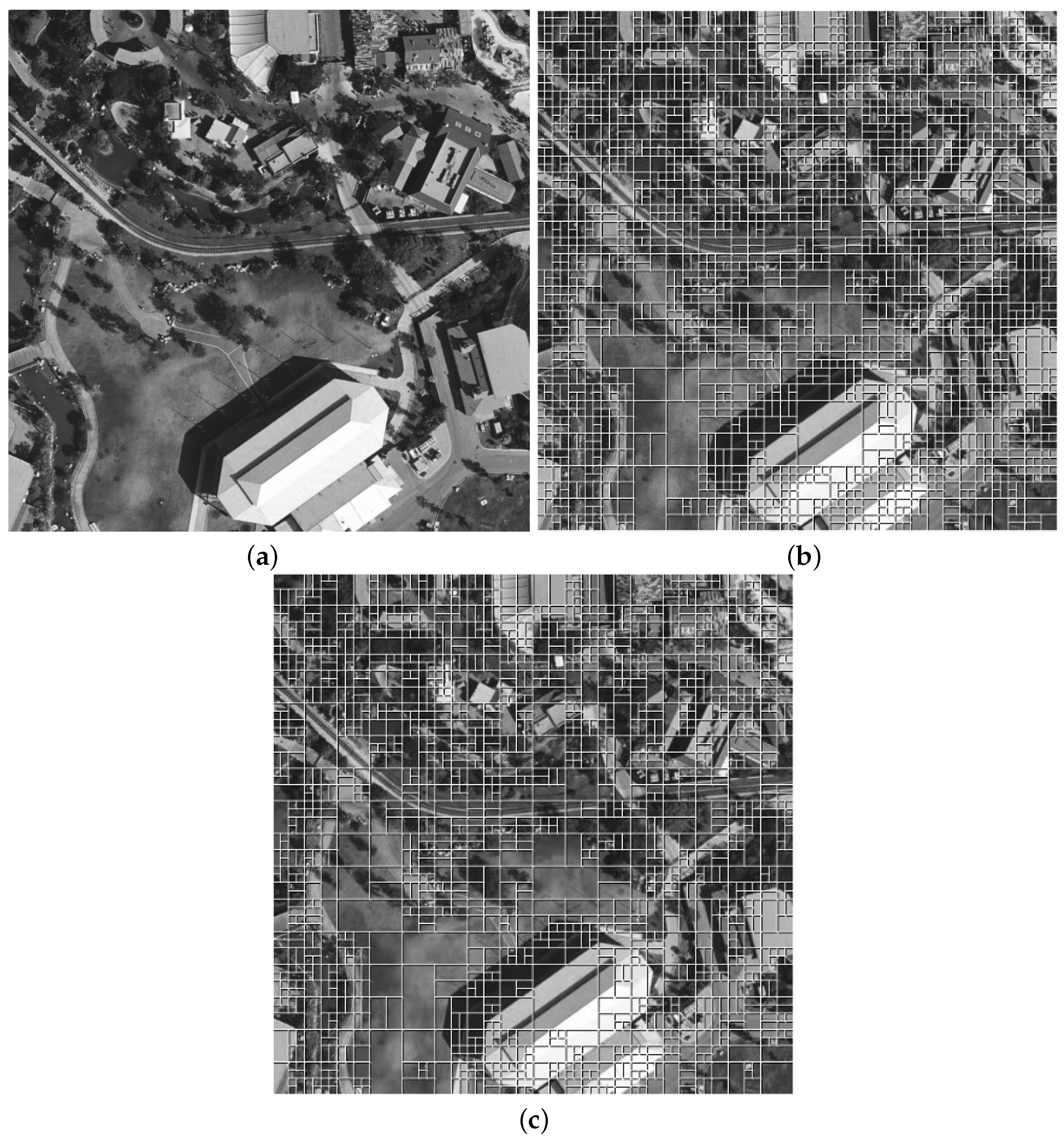
The map of
in blocks (magnified by 5 for better visualization) for the test image “Frisco” (
Figure 3a) is presented in
Figure 10a, whereas
Figure 10b shows the map of
in blocks (magnified by 28 for better visualization) for the same test image. It is clearly seen that
is smaller (pixels are darker) in homogeneous regions of the image where the values of
are smaller (the pixels are darker).
The scatter plots for other test images are very similar. The parameters of the fitted curves obtained using the approximation (
6) are presented in
Table 5. In comparison to the corresponding values in
Table 4, they are very similar. The only difference is that the values of the parameter
c for the ADCT coder are slightly larger. However, they are again approximately equal to QS/3.47 (1.44, 2.88, and 5.76 for QS equal to 5, 10, and 20, respectively).
Since a great number of
and
, corresponding to each other, are obtained for three values of QS, it is possible to obtain aggregate scatter plots for both considered coders. Furthermore, the scatter plots in a normalized way as the dependence of
vs.
are presented. For the coder AGU, the aggregated scatter plot is presented in
Figure 11. The general properties of this scatter plot are similar to those presented earlier. There is a monotonously increasing part of the fitted curve observed for
and the “saturation part” where
is close to unity that takes the place for
. The fitted curve is expressed as
Note that the value of the parameter c is not equal to 1, but it is quite close to unity.
Similarly, the aggregated scatter plot has been obtained for the ADCT coder. It is presented in
Figure 12. A comparison of the scatter plots in
Figure 11 and
Figure 12 shows that their main properties are quite close. Note that large ratios
relate to “very active” local areas (where sharp edges or large contrast small-sized objects are observed) and quite small QS values.
The largest variations of with respect to the fitted curves take place for . Such situations are observed for blocks that correspond to low-contrast edges, details, and textures that are the most typical for natural scene images.
The obtained fitted curve is given as
In this case, the value of the parameter c is even closer to unity.
5. MSE Prediction and Its Accuracy
Having obtained the expressions (
7) and (
8) for the AGU and ADCT coders, respectively, it is possible to predict
for each
k-th
pixels block of a given image using the corresponding estimate
obtained for this block.
For a given block and QS, one has
Assuming the knowledge of the estimates
where
K denotes the total number of blocks (the questions how the blocks can be positioned and what should be their number will be discussed later), the MSE for entire image can be predicted as
or
where
is the value of RMSE in a
k-th block determined by the Formula (
5). Note that it is very easy to calculate all
in advance if the block positions are known in advance as well.
Let us now analyze the accuracy of predicting the MSE for introduced distortions.
Table 6 presents the data for the four test images used in forming the scatter plots for the AGU coder. As it may be seen, the true values of the MSE are close to the corresponding predicted ones (
); the relative difference is considered small in practical applications as it does not exceed 10%. The data for the ADCT coder for the same four images are presented in
Table 7. Their analysis shows that the true and predicted values are also quite close. The maximal difference does not exceed 8%, i.e., 0.3 dB with regard to PSNR.
However, the results for images that have not been used in training (obtaining the fitting curves for the scatter plots) are more interesting. Such verification data have been obtained for 16 other test images of different origins. There are some traditional images such as “Lena”, “Baboon”, “Barbara”, “Boat”, “Goldhill”, “Peppers”, and “Man”. There are also highly textural images as “Grass” and “Bikes” (see small copies in
Figure 13). Several remote sensing images, such as “Frisco”, “Airfield” (both shown in
Figure 3), “Lu01”, “San Diego1”, “a13sm”, “Sent01”, and “Sent02” (see small copies in
Figure 13), have also been used. The goal of using images of different origins is to demonstrate that the proposed approach to prediction is applicable in different practical situations.
Selected results are presented in
Table 8 and
Table 9, where the most interesting examples are shown. Alongside with this, statistical results characterizing the accuracy of prediction are presented below.
An analysis of data in
Table 8 demonstrates the following. Firstly, for QS = 5, the MSE values do not differ significantly (they vary from 1.55 to 2.14), and they are predicted well. Secondly, for QS = 10, the difference in the MSE values increases (they vary from 4.2 for simple-structure image “Lu01” to 7.81 for the complex-structure image “Grass”), but the prediction is still considered accurate enough. Finally, for QS = 20, the MSE may differ noticeably depending on the image complexity (from 10.21 for “Lu091” to 30.92 for the test image “Grass”). However, the predicted values are in good agreement with the true MSE, and this happens for all of the images used in our analysis.
Bias and variance have been also determined for the true and predicted values for all twenty images used in analysis. For QS = 5, they are equal to −0.11 and 0.18; for QS = 10, they are equal to 0.07 and 0.51; and for QS = 20, they are equal to 2.77 and 8.66, respectively. The bias and RMSE constitute less than 15% of the mean values for each QS, and such a level of accuracy is acceptable in practice (in fact, the PSNR is predicted with a maximal error of less than 1.5 dB).
An analysis of data presented in
Table 9 shows the following. Firstly, if the QS = 5, the MSE values vary in rather narrow limits (from 1.69 to 2.14), and they can be predicted well enough. Secondly, when the QS = 10, the MSE values vary from 4.61 for the image “Lu01” having simple structure to 8.21 for the image “Grass” with the complex structure. The prediction accuracy is high for all of the images. Thirdly, when the QS = 20, the MSE can vary in wide range, e.g., from 11.25 for the image “Lu091” to 31.92 for the image “Grass”. The predicted values are quite close to the corresponding true ones, and, in fact, this takes place for all of the images employed in our study.
Concerning bias and variance, they are as follows: for QS = 5, they are equal to −0.15 and 0.019; for QS = 10, they are equal to 0.07 and 0.51; and for QS = 20, they are equal to to 2.77 and 8.66, respectively. The bias and RMSE constitute less than 16% of the mean values for each QS, and such a level of accuracy is acceptable in practice (in fact, the PSNR is predicted with maximal error less than 1.4 dB). A comparison of data in
Table 8 and
Table 9 shows that the values of MSE
pred for the ADCT coder are usually slightly larger than for the coder AGU. This conclusion can also be drawn from a comparison of expressions (
7) and (
8), where the value of the parameter
c is larger in the latter case.
Furthermore, the prediction accuracy for the method [
22] using the ADCT coder for QS = 20 has also been analyzed. The minimal predicted MSE is observed for the image “Lu01” (11.63), and the maximal (34.43) id observed for the test image “Grass”. The statistical analysis shows that the bias between the predicted and true values of the MSE is equal to −1.44, and the variance equals 7.11. This means that the prediction accuracy is of the same level as for the method proposed in this paper.
There are several aspects left for discussion. Firstly, all of the results presented above have been obtained for non-overlapping blocks fully covering the image area. Thus, for the pixels images used in our analysis, the calculation of has been employed. It is possible to expect that the use of overlapping blocks can improve the prediction. Thus, the fully overlapping blocks with their total number equal to 255,025 have been additionally used. However, this has not led to an improvement of the prediction accuracy. Moreover, the values of MSEpred corresponding to each other for the non-overlapping and fully overlapping blocks differ insignificantly—by less than 0.04%. For example, for the test image “Fr04” and Q = 20 (the AGU coder), the values of MSEpred are equal to 22.240 and 22.264 for non-overlapping and fully overlapping blocks, respectively. Furthermore, the case in which 1000 blocks have been placed randomly has been studied. The obtained prediction results practically do not differ from the corresponding data for non-overlapping blocks. Hence, there are some interesting options for accelerating the prediction by analyzing a limited number of blocks.
Starting from the developed method for predicting MSE, in practice one needs an algorithm for providing a desired value of MSE
des. Then, several options can be proposed. For example, in the first step, calculate the correcting factor as
and
then determine
If
is quite close to
(e.g., if they differ by no more than 10%), the value
may be used for final compression. If this condition is not satisfied, the final QS may be calculated as
and applied for compression.
The simplified flowchart of the proposed method is presented in
Figure 14.
This algorithm has been first tested for the coder AGU for MSEdes = 20 for all twenty images used in previous studies. The provided MSE varies from 11.87 (image “Barbara”) to 20.59 (image “Grass”), and its bias and variance are equal to 3.22 and 5.79, respectively; hence, this accuracy can be considered satisfactory. The final QS varies from 16.04 for the image “Grass” to 24.99 for the image “Frisco”, i.e., as expected, the final QS is the largest for simple-structure images and the smallest for complex-structure images. As one can see, the provided MSE is, on average, smaller than desired, and this mainly happens for simple-structure images. On one hand, this can be useful in practice since one has some “reserve” in quality just for images for which the distortions are more visible. On the other hand, it is possible to introduce some additional correction to remove the bias.
The proposed algorithm has been also tested for the ADCT coder for MSEdes = 20. The provided MSE varies in its limits from 12.06 for the image “Barbara” to 21.16 for the image “San Diego”. The bias and variance are equal to 2.86 and 6.46, respectively. So, again a bias and an RMSE of errors smaller than 15% have been obtained; such accuracy can be considered satisfactory. The final QS varies in its limits from 16.04 for the image “Grass” to 24.90 for the image “Frisco”.
The additional verification of the proposed algorithm has been made for 300 grayscale versions of
pixels images from the TAMPERE17 noise-free image database [
37]. The obtained results for MSE
des = 20 are presented in the form of histograms for AGU and ADCT coders in
Figure 15. In most cases, the provided MSE values are quite close to MSE
des = 20. Although the provided MSE values are shifted with respect to the desired MSE, and the variance of the final MSE is quite large, an important advantage is that the provided MSE values are mostly smaller than the desired MSE. The smallest provided MSE are observed for images with a simple and specific structure, e.g., those presented in
Figure 16. This phenomenon and its reasons are planned to be investigated in future research.
As can be seen, the algorithm of the determination of the final QS is computationally very simple. It requires the calculation of
twice, where the functions
are quite simple; the calculation of
; and elementary comparison and arithmetic operations. Being realized at Intel Core i7 L620 2.00 GHz with 8GB of RAM, it takes 0.363 ± 0.025 s for non-overlapping blocks for an image of size
pixels. Recall here that compression by AGU takes 1.020 ± 0.040 s (whilst decompression requires 1.735 ± 0.083 s). Thus, prediction is sufficiently faster than compression. Note that, additionally, it is possible to use a smaller number of analyzed blocks—if, e.g., 1000 blocks placed randomly are used instead of 4096 non-overlapping blocks, predicted MSEs differ by less than 1%; hence, such an approach is appropriate for practice. In this case, prediction can be realized by one order of magnitude less time than compression. The advantage of the proposed approach compared to [
22] is that it does not use the DCT in blocks and employs a minimal number of logical operations.
For the ADCT coder, the prediction time for non-overlapping blocks is 0.374 ± 0.065 s, whilst compression requires 3.080 ± 0.125 s, i.e., the prediction and determination of the final QS are considerably faster than the compression (decompression requires 1.998 ± 0.123 s). Certainly, the prediction can be additionally accelerated compared to the case of non-overlapping blocks by using a smaller number of blocks.
The obtained results have one more positive outcome. They allow one to propose the more adequate model (compared to [
38]) for simulating distortions due to lossy compression as spatially uncorrelated (white) Gaussian noise with variance dependent on image local activity.

 ,
, 


