Unlocking the Potential of Quantum Machine Learning to Advance Drug Discovery

Abstract

The drug discovery process is a rigorous and time-consuming endeavor, typically requiring several years of extensive research and development. Although classical machine learning (ML) has proven successful in this field, its computational demands in terms of speed and resources are significant. In recent years, researchers have sought to explore the potential benefits of quantum computing (QC) in the context of machine learning (ML), leading to the emergence of quantum machine learning (QML) as a distinct research field. The objective of the current study is twofold: first, to present a review of the proposed QML algorithms for application in the drug discovery pipeline, and second, to compare QML algorithms with their classical and hybrid counterparts in terms of their efficiency. A query-based search of various databases took place, and five different categories of algorithms were identified in which QML was implemented. The majority of QML applications in drug discovery are primarily focused on the initial stages of the drug discovery pipeline, particularly with regard to the identification of novel drug-like molecules. Comparison results revealed that QML algorithms are strong rivals to the classical ones, and a hybrid solution is the recommended approach at present.

1. Introduction

A complex and multifaceted endeavor that plays a critical role in advancing healthcare is drug discovery, which is the process of discovering new drugs and treatments. The goal of drug discovery is to identify and develop new drugs that can treat diseases and improve patients’ lives. The process involves a range of stages, including target identification, drug design and development, preclinical testing, clinical trials, and regulatory approval.

However, the drug discovery process is a laborious and protracted undertaking that often requires several years—more than a decade—of extensive research and development. Furthermore, it may necessitate an exorbitant amount of funding, often amounting to billions of dollars, before a molecule can ultimately obtain drug approval [1].

The advancements in computational chemistry techniques and the consequent increase in computer power have facilitated the emergence of computer-aided drug design (CADD) as an integral part of the drug discovery and development process [2]. The utilization of computers in pharmaceutical research has led to cost and time reductions in producing new drugs. Machine learning (ML)-based predictive models have further contributed to minimizing the cost and time of the drug discovery and development process. The availability of databases on multiple platforms containing millions of chemical compounds and their biological assay activities has also played a significant role in promoting the use of ML in drug discovery. Hence, the integration of computer-aided techniques and ML has revolutionized the field of drug discovery, making it more efficient and cost-effective.

Quantum computing (QC) is a type of computing that uses the principles of quantum mechanics to process information. Quantum computers utilize quantum superposition and entanglement to perform calculations, which exhibit tremendous potential in handling big data and expediting optimization algorithms prevalent in ML models. Unfortunately, manufacturing, controlling, and shielding quantum systems from noise pose significant technical difficulties, and the first prototypes have only emerged in the past decade. Despite the lack of hardware, mathematical analysis of algorithms is feasible, and the advent of high-performance quantum computer simulators, along with early prototypes in recent times, has propelled further research in this area. Moore’s Law describes the exponential growth in the processing power of classical computers, whose capabilities tend to double approximately every two years. However, it is expected that this trend will eventually reach its limits as transistors can no longer be scaled down further in the near future. On the other hand, Neven’s Law highlights the double exponential growth in computing power observed in quantum computers. These two observations underscore the immense potential and appeal of QC as a groundbreaking field.

Efficient training of classical machine learning models for complex problems, such as drug discovery, often necessitates access to high-speed computational resources. In recent years, certain researchers within the machine learning community have embarked on a study of the potential advantages that QC may offer within the realm of machine learning. The field that combines QC and ML to explore the potential benefits of using quantum computers for ML tasks is known as quantum machine learning (QML). Furthermore, the potential of QC in drug discovery has garnered significant interest from pharmaceutical and startup companies, as well as academia. This interest has led to numerous collaborations among these stakeholder groups, demonstrating a serious commitment to exploring the potential benefits of QC in the field [3,4].

The concept of using computers that comply with the principles of quantum mechanics to simulate quantum systems was initially proposed by Feynman [5] and later formalized by Lloyd [6]. One such system that can be simulated efficiently using quantum computers is quantum chemistry. Drug discovery, on the other hand, is a distinct area that benefits from advancements in both quantum chemistry and ML, which makes it one of the first fields to potentially integrate QC [7] and QML into its pipeline. However, achieving this objective is a daunting challenge, as quantum chemistry is a component of quantum mechanics but currently only runs on computers based on classical mechanics.

Presently, QML has demonstrated its significance in other areas of medicine, including precision medicine [8,9] and medical diagnostic systems [10,11,12,13,14,15,16]. In addition, several quantum algorithms, such as the variational quantum eigensolver (VQE) [17], have been employed in the drug discovery process.

An early study [7] examined the potential promises and limitations associated with integrating quantum computers and QML into the early phases of the drug discovery process. A review [18] with a similar structure to [7] has been conducted, which addresses the potential benefits and constraints of emerging QC technologies and QML in the domains of computational molecular biology and bioinformatics. The authors of the paper [19] presented significant progress in the development and utilization of QML techniques for various compounds and properties. They highlighted the essential breakthroughs achieved in this field and elucidated the challenges that remain to be addressed. The [20] review discussed QML, quantum chemistry, and quantum drug design, along with the associated challenges. In [21], the substantial potential of QC and QML for use in biology and medicine was presented, with the concept of a quantum advantage framework proposed to facilitate the development of quantum applications for researchers in biology and medicine. The review in [22] presented QC algorithms utilized in computational biology and in [23,24] in chemistry. Finally, [25] was the first review that explored QML models applied to the drug discovery pipeline.

In this review, the evolution of the use of QML algorithms in drug discovery is examined over the past five years. The following research questions were answered:

• Which QML models are used in drug discovery?
• Are QML versus ML algorithms more efficient in terms of time and accuracy in drug discovery?

In the rest of the paper, we present the background concepts in Section 2, we report the methodology in Section 3, the QML models in the drug discovery process are addressed in Section 4, a discussion is included in Section 5, and finally, we conclude our work in Section 6.

2. Preliminaries—Background

In order to understand the responses to the review questions posed in the previous section, it is essential to provide an overview of the terminology employed in the fields of drug discovery, QC, and QML.

2.1. Drug Discovery

Drug discovery refers to the complex process of transforming an initial hypothesis into a fully commercialized drug product. A significant portion of resources in drug discovery are devoted to identifying the molecule that exhibits significant drug activity against a disease, which is commonly referred to as a hit. Initially, a molecular target, typically a protein that regulates the outcome of a disease, is selected based on an idea to discover new pharmacomolecules to treat a specific pathological condition. Depending on the strategy followed, research is directed toward the discovery of an initial bioactive lead structure (hit) or a lead compound.

During the drug discovery stage, the pharmaceutical activity of a specific drug candidate or ligand is related to its ability to bind to the molecular target. To discover a lead structure or lead compound, a library of potential drug candidates is typically created and screened for their pharmaceutical activity. This is followed by the design, synthesis, and biological evaluation of a series of related compounds, also known as lead compounds, for optimizing the lead compound.

Throughout the drug discovery process, the physicochemical and pharmacokinetic properties of the substances are taken into account, initially computationally or through rapid measurements that provide a first estimate, such as high-throughput screening. Additionally, adverse effect rates are also considered. The final selected compounds then proceed to the next stages of drug development and clinical trials before one of them becomes a viable commercial product [2,26]. The drug discovery pipeline is presented in Figure 1.

The aforementioned process of drug discovery is an arduous and time-consuming endeavor that can take more than a decade and require billions of dollars before a molecule is eventually recognized as a drug. The cost and time associated with this process are dependent on the significant number of molecules that fail at various stages of the drug discovery pipeline, resulting in what is often referred to as big data. It is estimated that only one out of every five thousand drugs eventually reach the market, underscoring the high failure rate and the significant investment required [1].

In the drug discovery process, selecting a drug candidate involves meeting certain criteria, such as being potent, bioavailable, and nontoxic. With increasingly stringent requirements for efficacy, potency, and safety, the discovery of new drug-like molecules has become a complex and resource-intensive undertaking. However, recent advancements in computational approaches, bioinformatics, and the availability of 3D structures of molecular drug targets have accelerated the field of computer-aided drug design (CADD). This has led to the emergence of the term “in silico”, which describes a type of experiment that is performed virtually through computer simulations of biological processes [1].

In the design of new hit compounds or lead compounds, two primary techniques are utilized in computer-aided drug design (CADD) [2,27]: structure-based drug design (SBDD) and ligand-based drug design (LBDD). SBDD involves the use of knowledge regarding the 3D structure of the target protein at the molecular level to identify or design a potential chemical structure that will be used in the drug. In contrast, LBDD is employed when the structure of the target protein is unknown or cannot be predicted through available modeling methods. In this case, chemical similarity searches or the development of predictive quantitative structure-activity relationship (QSAR) models utilize knowledge of known active and inactive molecules.

2.2. Quantum Computing

Quantum computing (QC) is a rapidly evolving field that harnesses the principles of quantum mechanics, as opposed to classical computing, which relies on classical mechanics.

Qubit: In a quantum processor, information is stored in qubits, which are the quantum counterparts of classical bits. A qubit can be either |0〉 or |1〉 or simultaneously in any state between them (superposition) denoted as |ψ〉 = a|0〉 + β|1〉, where α and β are complex probability amplitudes. The states mathematically can be represented as 2-d vectors:

$$|0\rangle =[\begin{array}{c}1\\ 0\end{array}], |1\rangle =\left[\begin{array}{c}0\\ 1\end{array}\right], |\mathsf{\psi }\rangle =[\begin{array}{c}\mathsf{\alpha }\\ \mathsf{\beta }\end{array}].$$

Geometrically, qubits can be visualized using a sphere, called Bloch Sphere, as presented in Figure 2a. The Bloch sphere is a geometrical representation of a 3D Hilbert space of a quantum system’s state. To determine the state of a qubit, a common approach is to perform a projective measurement, which involves measuring the projection of its state vector along a specified axis, such as the z-axis, x-axis, or y-axis. The most fundamental projective measurement is performed on the computational basis, also known as the Z-basis. The Z-basis consists of the two basis states: |0〉 and |1〉, corresponding to the qubit’s state along the z-axis. A measurement in the Z-basis would correspond to projectors onto each of the two states. This measurement is represented on the Bloch sphere as follows: Upon completing the projective measurement, the qubit will collapse into one of its computational basis states. This process enables the extraction of information about the qubit’s state. The measurement operators are ${\mathrm{M}}_0=|0\rangle \langle 0|=\left[\begin{array}{c}1\\ 0\end{array}\right][\begin{array}{ccc}1& & 0\end{array}]=\left[\begin{array}{cc}1& 0\\ 0& 0\end{array}\right]$, and ${\mathrm{M}}_1=|1\rangle \langle 1|=\left[\begin{array}{c}0\\ 1\end{array}\right][\begin{array}{ccc}0& & 1\end{array}]=\left[\begin{array}{cc}0& 0\\ 0& 1\end{array}\right]$. Assuming the quantum system is initially in the state |ψ〉 = a|0〉 + β|1〉, the probability of measuring the system in state |0〉 according to the Born rule is:

$${\mathrm{P}}_0=\langle \mathsf{\psi }|{\mathrm{M}}_0^{†}{\mathrm{M}}_0|\mathsf{\psi }\rangle =\langle \mathsf{\psi }|0\rangle \langle 0|\mathsf{\psi }\rangle =({\mathsf{\alpha }}^{*}\langle 0|+{\mathsf{\beta }}^{*}\langle 1|)(|0\rangle \langle 0|)(\mathrm{a}|0\rangle +\mathsf{\beta }|1\rangle )={|\mathsf{\alpha }|}^2,$$

and in state |1〉 is P₁ = |β|². Furthermore, P₀ + P₁ = |α|² + |β|² = 1, as claimed by the Born rule. The state after measuring the system can be $|{\mathsf{\psi }}^{\prime }\rangle =\frac{{\mathrm{M}}_0|\mathsf{\psi }\rangle }{\sqrt{{\mathrm{P}}_0}}=\frac{\mathsf{\alpha }}{|\mathsf{\alpha }|}|0\rangle =|0\rangle$, where we implicitly ignore the irrelevant global phase factors $\frac{\mathsf{\alpha }}{|\mathsf{\alpha }|}$ or $|{\mathsf{\psi }}^{\prime }\rangle =\frac{{\mathrm{M}}_1|\mathsf{\psi }\rangle }{\sqrt{{\mathrm{P}}_1}}=\frac{\mathsf{\beta }}{|\mathsf{\beta }|}|1\rangle =|1\rangle$. It is important to note that a single measurement of a qubit only provides information about one specific basis state. Due to the probabilistic nature of quantum measurements, subsequent measurements of the same qubit may yield different outcomes. To gain a more comprehensive understanding of the qubit’s state, multiple measurements need to be performed (Figure 2b).

Superposition: The fundamental principle of QC is based on the concept of superposition. This allows certain operations to be run in parallel rather than sequentially, resulting in an exponential reduction of the number of operations required for certain algorithms.

Entanglement: In addition to superposition, another fundamental principle of QC is quantum entanglement. When a qubit is correlated with other qubits, a change or alteration to it affects the rest of the qubits, even if they are physically separated. The measurement of one entangled qubit can affect the behavior of the same measurement in other entangled qubits, regardless of the distance between them. While particles do not communicate in the classical sense, there is a statistical correlation between the results of their measurements that cannot be explained using classical physics.

Quantum Gate: A quantum gate is a basic quantum circuit that operates on a small number of qubits. A program or algorithm consists of many quantum gates, similar to classical logic gates. In contrast to classical gates, quantum logic gates are reversible and operate simultaneously in all possible states of the qubit instead of operating in a state of either 0 or 1. The most common single-qubit quantum gates are the Hadamard (H), Identity or Pauli I gate (I), Bit flip or Pauli X gate (X), Pauli Y gate (Y), Pauli Z gate (Z), and Rotation gates (RX, RY, RZ). The Pauli gates are also sometimes notated as σ_x, σ_y, σ_z, or with an index σ_i, so that σ₀ = I, σ₁ = X, σ₂ = Y, σ₃ = Z. The most common two-qubit gate is the controlled-Not (CNOT or CX).

The Hadamard gate facilitates the transformation of a qubit from a single computational basis state to a superposition state $\mathrm{H}=\frac{1}{\sqrt{2}}\left[\begin{array}{cc}1& 1\\ 1& -1\end{array}\right]$. The identity (I) gate, when applied to any arbitrary state, leaves the state unchanged $\mathrm{I}=\left[\begin{array}{cc}1& 0\\ 0& 1\end{array}\right]$. The X gate, in relation to the computational basis, performs an operation equivalent to the classical NOT operation. This gate interchanges the computational basis states, resulting in |0〉 becoming |1〉 and |1〉 becoming |0〉 $\mathrm{X}=\left[\begin{array}{cc}0& 1\\ 1& 0\end{array}\right]$. The X gate generates a half-turn in the Bloch sphere about the x-axis, while the Pauli Y gate generates a half-turn in the Bloch sphere about the y-axis $\mathrm{Y}=\left[\begin{array}{cc}0& -i\\ i& 0\end{array}\right]$, and finally the Pauli Z gate generates a half-turn in the Bloch sphere about the z-axis $\mathrm{Z}=\left[\begin{array}{cc}1& 0\\ 0& -1\end{array}\right]$. The rotation gates RX, RY, and RZ rotate the state vector by an arbitrary angle about the x-axis, y-axis, and z-axis in the Bloch sphere, respectively, where:

$$\mathrm{R}\mathrm{X}=\left[\begin{array}{cc}\cos (\frac{\mathsf{\theta }}{2})& -\mathrm{i}\sin (\frac{\mathsf{\theta }}{2})\\ -\mathrm{i}\sin (\frac{\mathsf{\theta }}{2})& \cos (\frac{\mathsf{\theta }}{2})\end{array}\right], \mathrm{R}\mathrm{Y}=\left[\begin{array}{cc}\cos (\frac{\mathsf{\theta }}{2})& -\sin (\frac{\mathsf{\theta }}{2})\\ \sin (\frac{\mathsf{\theta }}{2})& \cos (\frac{\mathsf{\theta }}{2})\end{array}\right], \mathrm{R}\mathrm{Z}=\left[\begin{array}{cc}{\mathrm{e}}^{-\mathrm{i}\frac{\mathsf{\theta }}{2}}& 0\\ 0& {\mathrm{e}}^{\mathrm{i}\frac{\mathsf{\theta }}{2}}\end{array}\right].$$

These gates rotate θ radians anti-clockwise about the x-axis, y-axis, and z-axis. In addition to gates that affect one qubit, there are many gates that use more than one qubit. For example, the CNOT gate acts on two qubits, where the first is the so-called control qubit and the second is the target qubit. If the control qubit is |1〉 then it will flip the target qubit state from |0〉 to |1〉 or from |1〉 to |0〉. Its matrix representation is as follows:

$$\mathrm{C}\mathrm{N}\mathrm{O}\mathrm{T}=\left[\begin{array}{cccc}1& 0& 0& 0\\ 0& 1& 0& 0\\ 0& 0& 0& 1\\ 0& 0& 1& 0\end{array}\right].$$

Quantum Supremacy: In many cases, analyzing the number of steps taken by quantum algorithms can show that they outperform classical algorithms for specific problems. This ability is known as quantum supremacy, where the number of steps taken by quantum algorithms is less than that taken by classical algorithms. The best-known examples of quantum acceleration include Shor’s algorithm for factorization, Grover search, and the simulation of quantum systems.

NISQ: NISQ (noisy intermediate-scale quantum) devices are quantum computers that implement logic operations using physical qubits and gates. Recent research has demonstrated that NISQ devices, which have a moderate number of qubits, can produce quantum states whose measurement results follow distributions that are difficult to produce by a classical computer [28]. While these devices will not be able to implement error correction, they are expected to provide computational advantages over classical supercomputers for certain problems [28]. It is important to note, however, that current quantum devices are still susceptible to noise and errors due to their interactions with the environment, which is a major obstacle to overcome to achieve scalable, fault-tolerant quantum computing (FTQC) devices.

Quantum Algorithm/Circuit: A quantum algorithm (QA), defined as a circuit, is composed of three essential parts (Figure 3a). The first part involves the conversion of classical data into quantum data, which is referred to as quantum embedding, state preparation, or feature mapping. The second part involves a sequence of quantum gates that are applied to the quantum data, resulting in a quantum computation. Finally, measurements are taken to extract classical information from the quantum system.

Variational Quantum Algorithm/Circuit (VQA/VQC): A variational quantum algorithm/circuit (VQA/VQC) is a type of hybrid quantum-classical optimization algorithm in which an objective function is evaluated by quantum computation [29]. The parameters of this function are then updated using classical optimization methods (Figure 3b). The terms “parameterized quantum circuit” (PQC) and “variational quantum algorithm” are used interchangeably.

2.3. Quantum Machine Learning (QML)

Quantum machine learning (QML) is a field that combines QC and ML to explore the potential benefits of using quantum computers for ML tasks. QML has gained significant attention as an emerging field owing to its potential to deliver superior performance over classical computers. However, due to the limited number of qubits available in current quantum computers, QML cannot be applied to real-world datasets at present.

As quantum computers reach their maximum computational capacity, they are expected to be able to process large amounts of data with unprecedented speed. This promises to unlock the full potential of QML, enabling it to deliver superior results across a wide range of ML tasks. Despite the challenges involved, QML represents a highly promising field with vast potential for future innovation and technological advancement.

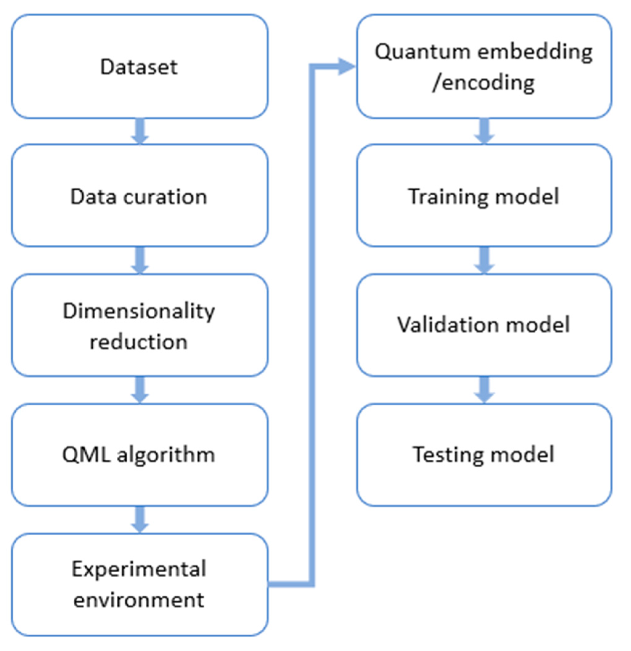
We present the workflow for the application of QML to diverse fields of study, which is illustrated in Figure 4. The workflow presented herein serves as a comprehensive framework for the deployment of QML techniques across diverse domains of study. Its primary purpose is to enable the seamless application of QML methodologies to a wide range of fields, thereby facilitating improved performance and outcomes in various tasks.

Dataset: The initial step in the QML process involves choosing a dataset with specific characteristics. Apart from physicochemical properties that contribute to absorption, distribution, metabolism, excretion, and toxicity, the dataset must have characteristics that allow easy production and handling in the laboratory. This is because the pharmaceutical industry typically focuses on small molecules rather than large proteins or complex compounds. To simplify the handling and analysis of the compounds of these small molecules, formats such as SMILES [30,31] and Morgan Fingerprint [32] are commonly utilized to represent their sequence and structure. These representations aid in simplifying the handling and analysis of small molecules in the context of ML algorithms.

In the realm of molecule datasets, there are two distinct approaches for describing the molecules. The first approach is based on the physical properties of the molecules, and datasets such as DrugBank, PubChem, ChEMBL, TOUGH-C1, PDBbind, and LIT-PCBA fall under this category. The second approach is based on the quantum chemical properties of the molecules, and datasets such as QM7, QM9, QM9-extended [33], QMugs [34], and PubChemQC follow this approach. However, there is currently a scarcity of data collections that provide a comprehensive description of large bioactive molecules along with their corresponding quantum chemical properties [34].

The dataset is partitioned into two subsets: a larger subset primarily used for training the model and a smaller subset exclusively used for testing the trained model’s performance.

Data Curation: The increasing diversity and complexity of data in QML applications pose new challenges for data quality issues such as noise, data imbalance (overrepresentation of either active or inactive molecules), outliers, unlabeled data, no-normalized data, or data with missing values. Low-quality data can significantly affect the accuracy and reliability of QML analysis. Therefore, it is crucial to properly curate the data before analysis [32].

Dimensionality Reduction: As previously stated, the use of NISQ computers, which are considered to be near-term QC devices, is limited due to the small number of qubits available. As a result, encoding large molecules is a challenging task. To address this issue, several dimension reduction techniques have been employed, including principal component analysis (PCA) [30,32,35], linear discriminant analysis (LDA) [32], Autoencoder [35], and Anova [30]. A fundamental inquiry arises as to which of these methods provides the most effective data compression while retaining the necessary information for the development of efficient prediction models.

QML Algorithm: The selection of a QML algorithm is a crucial decision that requires careful consideration. Various QML algorithms exist, each with its own unique strengths and limitations. It is essential to evaluate the specific requirements of the drug discovery and the characteristics of the available quantum hardware or quantum simulator before choosing an algorithm. Thorough research and analysis should be conducted to determine which QML algorithm would be most effective for the drug discovery process and the type of data available.

Experimental Environment: The evaluation of QML techniques requires careful consideration of the platform on which the algorithms will be executed. The execution of QML models can occur either on quantum simulators, such as IBM’s Qiskit, Google’s Cirq, Tensorflow, and PennyLane, or on real quantum processors, such as those offered by IBM, Google, Rigetti, Xanadu, IonQ, and D-Wave. In recent times, Amazon and Microsoft have introduced cloud-based applications that enable researchers to run quantum algorithms on different quantum processors. Consequently, the choice of platform for executing QML algorithms is a crucial aspect that impacts the reliability and performance of QML techniques.

Quantum Embedding: Quantum embedding is a fundamental constituent of QML that entails the encoding of classical data into quantum states. It is of utmost importance, as all data present in natural phenomena and databases is classical. Therefore, quantum embedding serves as a bridge between classical data and quantum algorithms, enabling the use of QML techniques to address real-world problems. The computational cost of QML algorithms is directly affected by the choice of quantum embedding strategy. Despite the various strategies available, there is still much ongoing research regarding the transformation of classical data into a quantum circuit. Notably, amplitude embedding [35,36], angle embedding [31,36,37,38,39,40], and Hamiltonian [41] are the common encoding methods.

In the amplitude embedding approach, data is encoded into the amplitudes of a quantum state. A normalized classical N-dimensional datapoint x is represented by the amplitudes of a n-qubit quantum state |ψ_x〉 as $\left|{\mathsf{\psi }}_{\mathrm{x}}\right.〉={\sum }_{\mathrm{i}=1}^{\mathrm{N}}{\mathrm{x}}_{\mathrm{i}}\left|\mathrm{i}\right.〉$, where N = 2ⁿ, x_i is the i-th element of x, and |i〉 is the i-th computational basis state. For instance, suppose we want to use amplitude encoding to encode the data point x, which has four dimensions (x₁ = 1.2, x₂ = 2.7, x₃ = 1.1, x₄ = 0.5). We require two qubits for these four features of x. The first step is to normalize the input ${\mathrm{x}}_{\mathrm{n}\mathrm{o}\mathrm{r}\mathrm{m}}=\frac{1}{\sqrt{10.19}}$ (x₁ = 1.2, x₂ = 2.7, x₃ = 1.1, x₄ = 0.5), where 10.19 = 1.2² + 2.7² + 1.1² + 0.5² and the final quantum state is $\left|{\mathsf{\psi }}_{\mathrm{x}\mathrm{o}\mathrm{r}\mathrm{m}}\right.〉=\frac{1.2}{\sqrt{10.19}}\left|00\right.〉+\frac{2.7}{\sqrt{10.19}}\left|01\right.〉+\frac{1.1}{\sqrt{10.19}}\left|00\right.〉+\frac{0.5}{\sqrt{10.19}}\left|00\right.〉$.

Angle encoding, also referred to as tensor product encoding, is a technique used to perform angle embedding by applying rotations on the x-axis, y-axis, or z-axis using quantum gates (RX, RY, and RZ). It requires n qubits to represent n-dimensional data x. $\left|{\mathsf{\psi }}_{\mathrm{x}}\right.〉={\otimes }_{\mathrm{i}=1}^{\mathrm{n}}\mathrm{R}\left({\mathrm{x}}_{\mathrm{i}}\right)\left|0^{\mathrm{n}}\right.〉$, where x_i is the i-th element of x, and R can be one of RX, RY, or RZ. The Hamiltonian encoding is a linear combination of the tensor product of Pauli operators $\mathrm{H}={\sum }_{\mathrm{j}}{\mathrm{C}}_{\mathrm{j}}{⨂}_{\mathrm{i}}{\mathsf{\sigma }}_{\mathrm{i}}^{\left(\mathrm{j}\right)}$, where C_j is a scalar coefficient and σ_i represents an element of the Pauli group {I, X, Y, Z}. An example of Hamiltonian encoding is H = 4.5I + 2.1X − 1.6ZZ.

Training and Validation Model: In order to ensure the validity of the model with unknown data, it is essential to avoid overtraining during the training phase of the algorithm. To accomplish this, multiple runs of the algorithm are performed using the training data. It is common practice to employ techniques such as cross-validation (CV) in such cases. Cross-validation provides a means to measure the degree of generalization of the model during training, assess its performance, and estimate its performance with unknown data. The cross-validation process involves the splitting of the original dataset into two subsets: the training set and the validation set. This procedure is repeated in each run of the experiment. The training set is used to train the model, while the validation set is used to assess its performance. By repeating this process, the algorithm can be trained and tested on different subsets of the data, which helps reduce the impact of any potential biases in the data. The performance of the model is evaluated by calculating metrics such as accuracy, precision, recall, and F1-score, which are commonly used in ML.

Testing Model: After training the model with the training set and tuning the parameters using the validation set, it is necessary to evaluate the model’s ability to generalize well to new and unseen data. The process of testing the model against the test set and assessing its performance using appropriate statistical measures is critical to determining the effectiveness of the model. If the test results demonstrate statistical significance, it can be concluded that a new and predictive drug model has been successfully developed. This approach ensures that the model’s performance is not limited to the data it was trained on and can be applied to real-world scenarios. Therefore, testing the model with the test set is a crucial step in validating the effectiveness of the model.

2.4. Quantum Machine Learning (QML) Algorithms

This section presents an introduction to QML algorithms. During the initial stages of QML research, the primary objective was to convert classical ML algorithms into their quantum counterparts. Several of these quantum algorithms have yielded promising outcomes in data processing. Most QML algorithms are variational quantum algorithms (VQAs), where the parameters of the quantum circuit are updated through classical optimization methods.

2.4.1. QNN

Quantum Neural Network (QNN): Neural networks (NNs) are algorithmic models that are inspired by the functioning of the human brain. They can be trained to recognize patterns in data and solve complex problems. The classical NNs are based on a series of interconnected nodes, or neurons, that are organized in a layered structure. These neurons have parameters that can be learned through the application of an ML algorithm. The implementation of QNNs does not rely on strict definitions of concepts such as “quantum neuron” or what constitutes the “quantum layer” of a classical NN. The architectural differences between classical NNs and quantum NNs can be observed in Figure 5a,b. One of the greatest challenges in QNNs is the disparity between the nonlinearity of classical NNs and the linearity of QC. Another significant challenge for optimizing QNNs is the initialization of their parameter space, as indicated in [42]. Several implementations of QNNs can be found in references [43,44,45].

Quantum Convolutional Neural Network (QCNN): A convolutional neural network (CNN) is a crucial category of NN designed for image classification. The architecture of a CNN typically includes several layers, each of which performs a specific type of computation. The first layer is usually a convolutional layer, which applies a set of filters to the input image to extract specific features. The second layer is typically a pooling layer, which downsamples the output of the convolutional layer to reduce the dimensionality of the feature map. Subsequent layers may include additional convolutional and pooling layers, followed by one or more fully connected layers that classify the input based on the extracted features (Figure 6). The primary goal of classical CNN and QCNN is to reduce the size of the matrices associated with images, which can be extensive. The first attempts to implement a QCNN were made in [46,47], where novel approaches were introduced. These pioneering works represent a significant step towards the development of efficient and effective QCNNs for image classification tasks and have inspired further research in this area.

Quantum Long Short-Term Memory (QLSTM): QLSTM is a type of quantum recurrent neural network (QRNN). Recurrent neural networks are designed to maintain the temporal storage of information. This is achieved using recurrent connections within the network, which allow the network to maintain previous states of information. In QLSTMs, variational quantum circuits are utilized to perform the recurrent computation within the network, replacing the traditional recurrent connections used in classical RNNs. These variational quantum circuits are designed to be trainable using techniques such as quantum gradient descent, which allows the network to learn from data. Initial attempts to implement hybrid QLSTMs were made by [31,48], both of which used variational quantum circuits in their QLSTM models.

Quantum Radial Basis Function Neural Network (Q-RBFNN): Q-RBFNN is a type of QNN architecture that shares similarities with the classical RBFNN. The RBFNN is composed of an input layer, a single hidden layer, and an output layer, and it utilizes radial basis functions as activation functions within the hidden layer.

Quantum Boltzmann Machine (QB)/Quantum Restricted Boltzmann Machine (QRBM): The Boltzmann machine (BM) is a stochastic neural network with two types of neurons—visible (inputs and outputs) and hidden—that are interconnected with one another. The quantum BM is represented as a set of interacting quantum spins that correspond to a tunable Ising model. In restricted Boltzmann machines (RBMs), visible neurons connect to hidden neurons without any synapses between identical neurons. In other words, visible neurons do not connect with other visible neurons, and hidden neurons do not connect with other hidden neurons. The analysis of QBMs conducted by Amin et al. [49] holds substantial significance and serves as a seminal study that has laid the groundwork for further research in the field.

2.4.2. QGAN

Quantum generative adversarial networks (QGANs) are the quantum analog of classical generative adversarial networks (GANs). The goal of the GANs is to generate data that resembles the original data used in training. It consists of two neural networks, a generator and a discriminator, which are trained. The generator creates fake data that mimics the real training dataset, whereas the discriminator tries to distinguish the real from the fake data. During the training process, both neural networks iteratively improve each other. In the end, the generator should create new data very close to the training data set (Figure 7). The present literature review [50] provides a comprehensive exposition on quantum generative adversarial networks (QGANs).

2.4.3. QVAE/AE

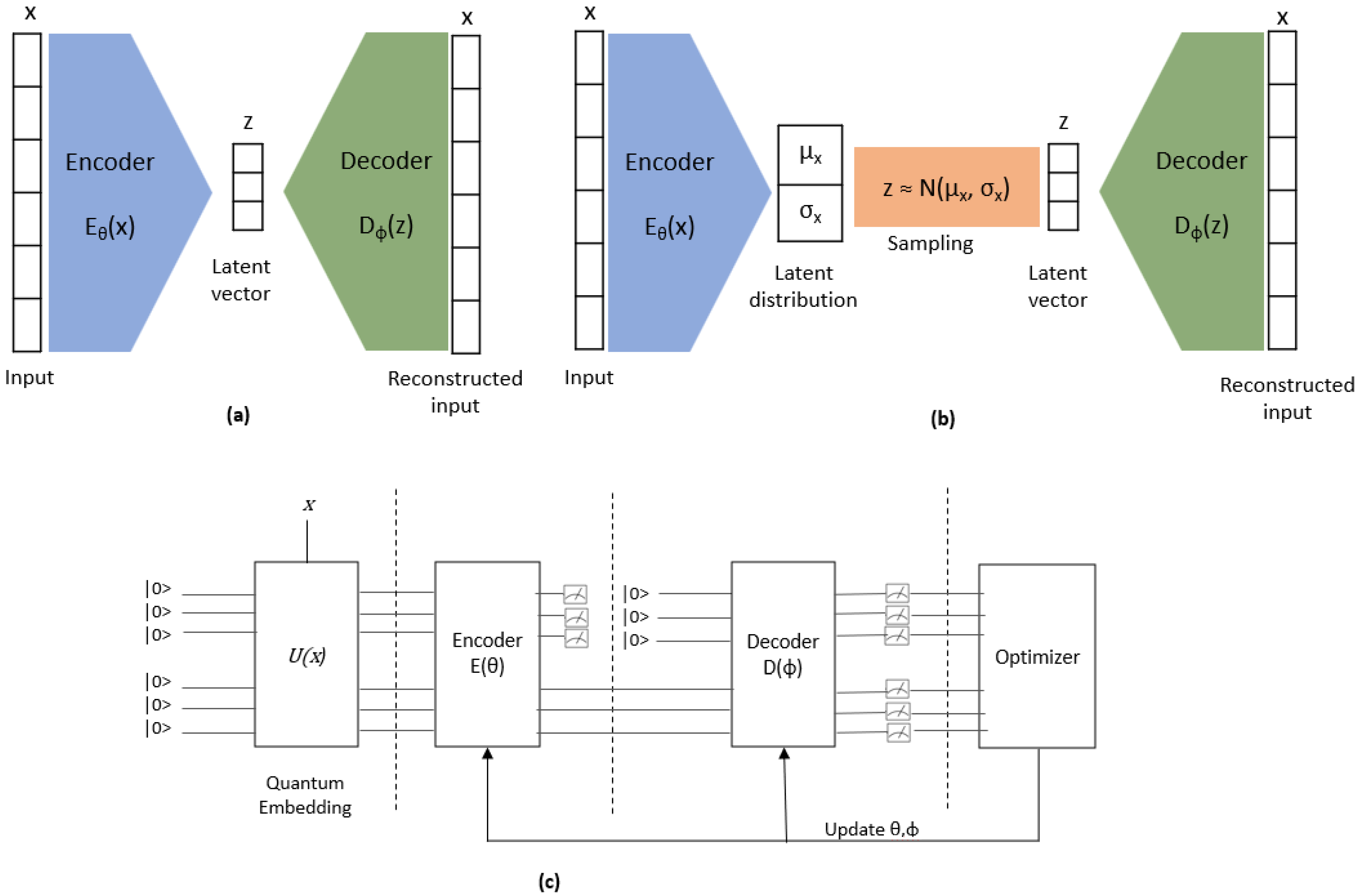
Autoencoder (AE) is an unsupervised learning algorithm that comprises two components: an encoder and a decoder. The purpose of the encoder is to compress data from a higher-dimensional space to a lower-dimensional space, which is commonly referred to as the latent space. On the other hand, the decoder is responsible for converting the compressed data from the latent space back to the higher-dimensional space. The primary objective of the decoder is to recreate or reconstruct the input data with minimal loss of information from the latent space (Figure 8a).

Variational autoencoder (VAE), on the other hand, is an extension of the traditional AE algorithm. VAE encodes input data as a distribution in the latent space rather than a single point. Specifically, the encoder outputs both the mean and the standard deviation for each input. The latent vector is then sampled from this mean and standard deviation, which are subsequently fed to the decoder to recreate or reconstruct the input. The decoder in VAE works similarly to the one in AE (Figure 8b).

The initial endeavors to implement quantum autoencoder (QAE) and quantum variational autoencoder (QVAE), denoted by [51,52], respectively, are presented in this work. A comprehensive architecture of QAE/VAE is depicted in Figure 8c.

2.4.4. QSVM

The quantum support vector machine (QSVM) is a supervised ML algorithm utilized for binary classification tasks. The primary objective of this algorithm is to identify a hyperplane that can efficiently distinguish between the two classes and act as a decision boundary for future classification tasks. The optimal hyperplane is determined based on its maximum distance to the closest data points, which are referred to as support vectors (Figure 9). One of the distinguishing features of SVMs is their ability to work effectively even with non-linearly separable data sets. This is achieved through the use of a technique known as the “Kernel Trick”, whereby the data is transformed from a lower-dimensional space into a higher-dimensional space using specific functions. Ref. [53] provides further details on the QSVM algorithm.

2.4.5. Quantum Genetic Algorithms

Genetic algorithms (GA) are a subtype of evolutionary algorithms (Figure 10). In machine learning, they refer to a class of adaptive heuristics or search engine algorithms used to find solutions to search and optimization problems. It is a methodology that employs natural selection to solve unconstrained and constrained optimization problems. The quantum genetic algorithm (QGA) is a novel evolutionary algorithm that combines quantum computation with conventional genetic algorithm technology. In reference to the study of QGA, it is notable that one of the earliest works in this field can be found in reference [54].

2.4.6. Quantum Linear and No-Linear Regression

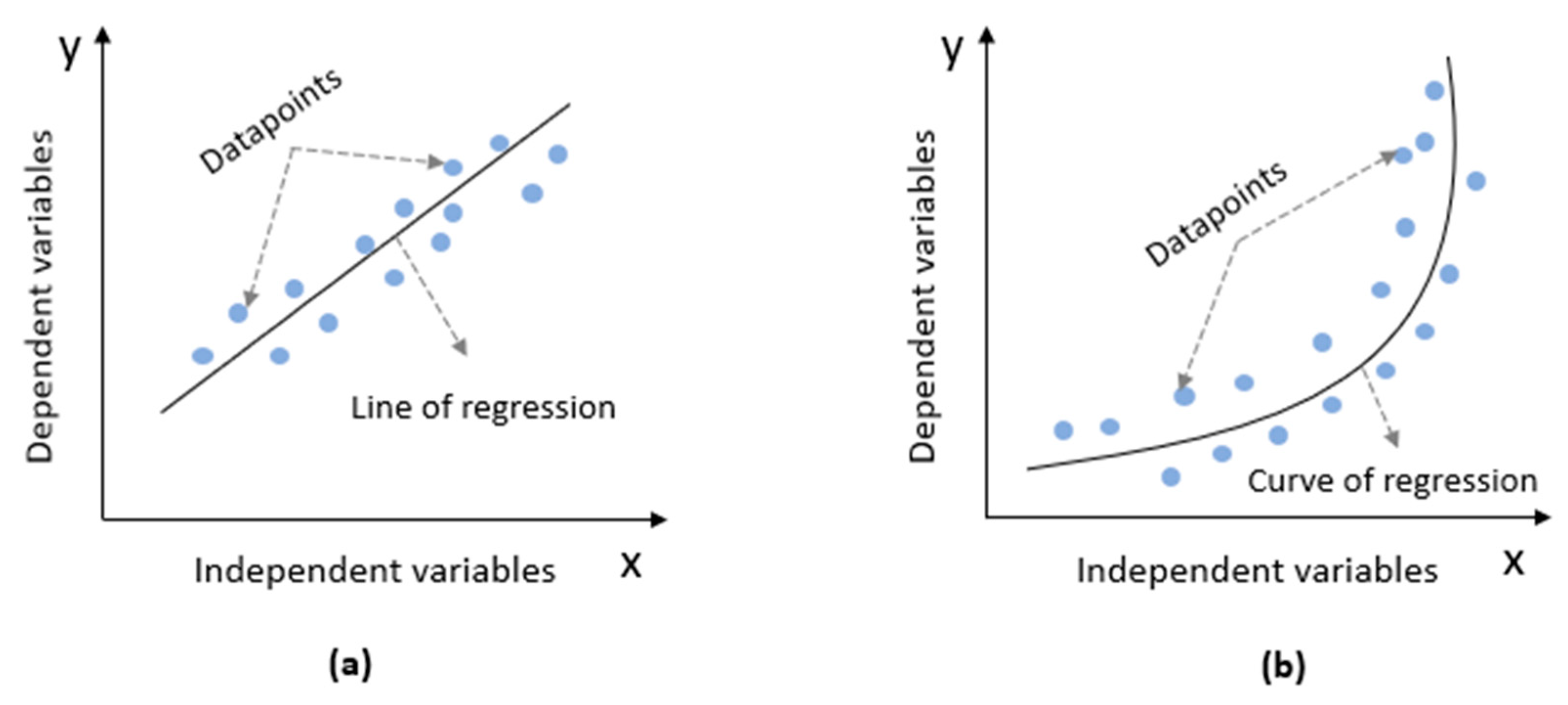
A regression model is a statistical model that describes the relationship between a dependent or response variable and one or more independent variables. It provides a function that can be used to predict the response variable based on the values of the independent variables. Linear regression (Figure 11a) is a type of regression analysis that finds the optimal linear relationship between the independent variables and dependent variables. This is achieved by minimizing the sum of the squared differences between the observed values and the predicted values. Nonlinear regression (Figure 11b) is a form of regression analysis in which the observational data are modeled by a function that is a nonlinear combination of the model parameters and depends on one or more independent variables. In contrast to linear regression, the function used in nonlinear regression is not linear, and the parameters are estimated using iterative methods of successive approximations. Nonlinear regression is useful for modeling complex relationships between variables where the relationship cannot be adequately described by a linear function.

3. Methodology

In this study, we employed the Preferred Reporting Items for Systematic Reviews and Meta-Analyses (PRISMA) 2020 methodology [55] to obtain a comprehensive understanding of the potential applications of QML in the drug discovery and design pipeline. PRISMA is commonly used in systematic reviews, but it can also serve as a foundation for reporting bibliographic reviews in other types of research, as is the case in our study.

This study focused on the application of QML algorithms to drug discovery and design and covered a period of five years. A comprehensive search was conducted in various databases, including Scopus, Springer, ACM, PubMed, ScienceDirect, Wiley Online Library, MDPI, IEEE Explore, Nature, RSC, IopScience, and ACS, to identify relevant articles. An advanced search filter was used in each database to limit the search results to articles written in English and published between January 2017 and March 2023. The search query was constructed using logical statements.

• “quantum machine learning” AND (“drug discovery” OR “drug design” OR “drug development”)

The study involved a search of 12 databases using the specified filters, which yielded a total of 517 articles. Duplicate articles were identified and removed, leaving 450 articles. The titles and abstracts of the remaining articles were examined, and those that were not related to the field of study were excluded, resulting in 34 articles. The full content of each of these 34 articles was reviewed to determine their relevance to the study. Six additional articles were included due to their relevance to the study but were not captured in the initial search. The process was illustrated using the PRISMA 2020 flowchart template and ultimately resulted in a final selection of 40 articles that met the research criteria (Figure 12).

The decrease in the number of papers studied can be attributed to the ambiguity of the term “quantum machine learning” (QML). It should be noted that in the present study, QML specifically refers to ML algorithms implemented on quantum computers. However, in some other papers, the term QML is used to describe classical ML algorithms applied to drug molecules encoded with the principles of quantum mechanics (QM). This difference in definition has resulted in the exclusion of certain papers from the study that do not align with the specific focus of the present research.

4. QML Applications in Drug Discovery

This section presents an overview of QML techniques used in drug discovery, including a comparison table per category. Each algorithm was compared either with its corresponding classical counterpart or with other quantum or hybrid algorithms, based on the respective studies. The purpose of these tables is to provide readers with a brief comparison of the algorithms. In each cell, the “+” symbol indicates that the quantum algorithm in the line is better than the algorithm in the column in terms of metrics such as accuracy; the “−” symbol indicates that it is worse; and “≈” indicates that they are about the same. Furthermore, in each cell of the table, a triplet of characteristics is reported, namely the datasets used, the running environment, and all metrics (

Table 1. QNN comparison (Part 1).

	NN	LSTM	QBi-LSTM	LNS, CNNWEF, RNN, and ATT-RNN
Weighted mQNN, cQNN, and qisQNN	[56] [≈] Precision [GenoDock, Platinum]/ [Rigetti, ibmq_bogota, PennyLane’s, Simulation]/ [AUC, F1, Sensitivity, Precision]
QLSTM		[31] [−] Training accuracy [31] [+] Testing accuracy [USPTO-50k]/ [simulation PannyLane]/ [accuracy, Loss]
QBi-LSTMA		[57] [+] Performance [TwiMed, TwitterADR]/ [simulation]/ [Precision, Recall rate, F1-score]	[57] [+] Performance [TwiMed, TwitterADR]/ [simulation]/ [Precision, Recall rate, F1-score]	[57] [+] Accuracy [57] [+] Training time [TwiMed, TwitterADR]/ [simulation]/ [Precision, Recall rate, F1-score]

,

Table 2. QNNs comparison (Part 2).

	RBFNN	H-QFT-Based Hybrid QNN	Single-Layer CNN + MLP	Linear Regression/Logistic Regression/SVM Random Forest/XGBoost/Neural Network
Q-RBFNN	[35] [≈] Accuracy [QM7]/ [simulation with noise]/ [MAE, RMSE, R2, Pearson correlation]
H-QNN		[35] [−] Accuracy [QM7]/ [simulation with noise]/ [L1-Loss]
single-layer QuanNN + MLP			[37] [+] Accuracy [TOUGH-C1]/ [simulation]/ [Cross Entropy]
QRBM				[41] [≈] Accuracy [Kuner,Golumbic]/ [D-Wave]/ [accuracy]

,

Table 3. QGAN comparison.

	MolGAN	QGAN-HG
QGAN-HG	[37,39] [+] Training epochs [37,39] [−] Training time [QM9, moderately reduced parameters]/ [Simulation,ibm_quito]/ [Fréchet Distance/training epochs/time]
QGAN-HG	[37,39] [−] Training epochs [37,39] [−] Training time [QM9, highly reduced parameters]/ [Simulation, ibm_quito]/ [Fréchet Distance/training epochs/time]
P-QGAN-HG		[39] [+] Learning accuracy [39] [+] Training time [37,39] [+] Training epochs [QM9, highly reduced parameters]/ [Simulation,ibm_quito]/ [Fréchet Distance/training epochs/time]

,

Table 4. QVAE/AE comparison.

	VAE/AE	VAE
BQ-VAE/AE	[36] [−] Accuracy [36] [≈] time training (epochs) [QM9] [non-normalized molecule]/ [simulation]/ [ accuracy, time training (epochs)]
BQ-VAE/AE	[36] [−] Accuracy [36] [+] time training (epochs) [QM9] [normalized molecule]/ [simulation]/ [accuracy, time training (epochs)]
SQ-VAE/AE	[36] [+] reconstruction accuracy [36] [+] sampling accuracy [PDBbind]/ [simulation]/ [accuracy, time training (epochs)]
Hybrid QVAE		[37] [−] Time learning [TOURCH1]/ [simulation]/ [L2 Loss, time]

,

Table 5. QSVM comparison.

	SVM	H-QSVM	Data Re-Uploading Classifier on CC
QSVM	[32] [−] Accuracy [SARS-CoV-2 (Vero cell), small dataset]/ [ibmq_rochester]/ [Accuracy]	[32] [+] Accuracy [SARS-CoV-2 (Vero cell), small dataset]/ [ibmq_rochester]/ [Accuracy]
QSVM	[30] [+] ROC in cases [LIT-PCBA, COVID-19]/ [simulation]/ [ROC] [30] [+] ROC in cases [ADRB2, COVID-19]/ [IBM Quantum Montreal, IBM Quantum Guadalupe]/ [ROC]
Data Re-uploading Classifier on QC			[32] [−] Accuracy [32] [+] Time [M. tuberculosis Inhibition -small dataset]/ [ ibmq_rochester]/ [accuracy, run time] [32] [−] Accuracy [32] [+] Time [cathepsin B(Pubchem)/ Krabbe disease (Pubchem)/ plague (Pubchem)/ M. tuberculosis (Pubchem)/ hERG]/ [simulation]/ [accuracy, run time]

,

Table 6. QIGP comparison.

	CGP and RBF-NN
QIGP	[40] [+] Accuracy [40] [+] Τime [221 phenols]/ [simulation]/ [R, cosine similarities, MSE]

and

Table 7. Quantum linear/No-Linear comparison.

	Classical Linear Regression	MLR/RBF-NN
Q Linear Regression	[35] [≈]Accuracy [QM7]/ [simulation with noise]/ [MAE, RMSE, R2, Pearson correlation]
PQC No Linear Regression		[38] [+] performance [221 phenols/ [simulation]/ [Rtrain2, Rval2, MSEtrain, MSEval RMStrain, RMSval]

).

4.1. QNN

In their study, Lau et al. [56] introduced a hybrid classical-quantum workflow, called HypaCADD, for use in CADD. This workflow aims to identify ligands that can bind to proteins while also accounting for genetic mutations that may affect drug binding. HypaCADD combines classical molecular docking, binding affinity prediction, and molecular dynamics with QML to predict the effects of mutations on drug binding. To evaluate the performance of HypaCADD, three QNN algorithms were benchmarked, including the weighted mQNN based on the margin classifier recommended by PennyLane, the qisQNN from Qiskit, and the custom QNN (cQNN) architecture based on the Farhi and Neven (FN) model. Initially, the researchers validated their method using the HCoV-229E 3CL^pro protein. Then, they applied HypaCADD to identify ligands that could bind with high affinity to SARS-CoV-2 virus proteins (3CL^pro) and remain resilient against various mutations in the target protein. From a dataset of over 11 million compounds, the team subsampled 30,000 compounds and identified two lead compounds, ZINC000016020583 and ZINC000036707984, as potential inhibitors. They compared the performance of the above QML algorithms with classical neural networks and demonstrated that QC was on par with classical computing. Overall, the results indicate that HypaCADD is a promising hybrid approach that integrates classical and QC to address the challenges of CADD, particularly in the identification of ligands that can bind to target proteins while accounting for genetic mutations.

Additionally, Beaudoin et al. [31] proposed a quantum long short-term memory (QLSTM) approach for chemical retrosynthesis, which is a crucial step in drug discovery. Chemical retrosynthesis aims to determine the reactants that can be combined to synthesize the final molecule by breaking it down into smaller parts. QLSTM is a quantum-classical hybrid approach and uses four variational quantum circuits (VQCs), which are quantum circuits with gate parameters trained classically. To evaluate the performance of QLSTM and compare it with classical long short-term memory (LSTM), the team used the USPTO-50k dataset and introduced two approaches to simplify the retrosynthesis process. Firstly, they selected a single reaction type from the ten in the dataset, and secondly, they included all reaction types (10) and selected two common chemical chains—acetic acid and acetone—and reduced the input reactions to only options that produce the selected chemical chains. The results showed that while the training accuracy of QLSTM (80%) was inferior to that of LSTM (100%), the accuracy of QLSTM (80%) surpassed that of classical LSTM (70%) in testing. In general, the study presented QLSTM as a viable tool and quantum-classical hybrid approach for chemical retrosynthesis. The results indicate that QLSTM has the potential to improve the accuracy of retrosynthesis predictions, which is a crucial step in drug discovery.

In their study, Wang et al. [58] proposed a novel approach, the quantum bi-directional long short-term memory with attention (QBi-LSTMA), for predicting adverse drug reactions (ADRs) in the context of drug combinations from big social network data. ADRs are a major challenge in drug discovery, and they remain a leading cause of morbidity and mortality. The attention mechanism used in the model imposes additional constraints on the QBi-LSTM architecture, ensuring that the semantic meanings of the data are rigorously matched. The model comprises six variational quantum circuits (VQCs), and its network structure has been simplified while retaining the primary topology of LSTMA. To evaluate the performance of QBi-LSTMA, the authors used data from Twitter, specifically, the TwiMed and TwitterADR datasets, for both training and testing. Their findings showed that while the performance in the training set was slightly better than that in the testing set, the QBi-LSTMA model’s performance was superior to that of Bi-LSTM and QBi-LSTM. The proposed approach outperformed other methods used for ADR prediction, such as LNS (linear neighborhood similarity), CNNWEF (word embedding features), RNN (recurrent neural network), and ATT-RNN (attention-based recurrent neural network).

Furthermore, Reddy and Bhattacherjee [35] presented a detailed methodology for predicting molecular atomization energies using various QML models. The authors benchmarked (a) the quantum and classical radial basis function neural networks (Q-RBFNN) and (b) the hybrid quantum neural network and QFT-based hybrid QNN. To simulate the behavior of NISQ systems, multivariate Gaussian noise (Δ) of mean 0 and covariance 0.1 was added to the QM7 dataset. The authors successfully trained the Q-RBFNN model and achieved similar results to those obtained from the classical RBFNN model. The performance of the QFT-based hybrid QNN model was found to be superior to that of the standard hybrid QNN model, indicating that the Fourier basis states provide a better representation of the data compared to the standard basis states.

Lastly, Li et al. [37] proposed a quantum neural network called the quantum convolutional neural network (QuanNN) for the purpose of classifying binding pockets in proteins. The TOUGH-C1 dataset was used to classify the pockets, which were represented as images, into one of three categories: nucleotide binding, heme-binding, or other. The implementation of the QuanNN model was performed using the Pennylane and PyTorch platforms. The QuanNN model, which consists of a single layer, was combined with Multi-Layer Perceptrons (MLP) for improved classification accuracy. The results showed that the QuanNN + MLP model outperformed single-layer CNN + MLP in terms of training and validation accuracy.

Jain et al. [41] introduced a cancer biomarker that utilizes a QRBM classifier to differentiate between two subtypes of non-small cell lung cancer: adenocarcinoma and squamous cell carcinoma. The model was developed using the D-Wave 2000Q quantum computer and trained on a dataset consisting of 104 patients that were curated from the Kuner and Golumbic datasets. Feature selection was performed using XGBoost. The main objective of the model is to enable precision medicine, which aims to identify the specific subtype of cancer a patient has in order to determine the optimal treatment. Additionally, precision medicine has the potential to influence drug design. Although the study did not aim to demonstrate quantum supremacy, the authors noted that the proposed model yielded favorable results, with classical methods performing similarly.

Geraci et al. [58] presented a quantum Boltzmann machine (QBM) approach that was implemented on the D-Wave quantum computer for predicting the response or non-response of placebo patients in central nervous system (CNS) clinical trials, with a specific focus on mood disorders such as major depressive disorder (MDD) and bipolar disorder. The rationale behind developing this model was the need to address the issue of placebo responders potentially obscuring actual positive results. The QBM model achieved a noteworthy prediction accuracy of 89% for identifying non-responders, but the accuracy for predicting responders was comparatively lower at 71%.

4.2. QGAN

Li et al. proposed a quantum generative adversarial network with a hybrid generator (QGAN-HG) [37,39] and a classical discriminator for drug discovery. The QM9 dataset was used in their experiments. The hybrid generator consists of a parameterized quantum circuit and a classical deep neural network to generate molecular structures represented by an atom vector and bond matrix. Synthetic molecules were then fed into the classical discriminator for classification as real or fake, and drug properties were evaluated using RDKit. To evaluate the expressive power of the hybrid generator, the number of neural network parameters was reduced to two levels: 85.07% (moderately reduced) and 98.03% (highly reduced). QGAN-HG with moderately reduced parameters and the original MolGAN achieved a reasonably good training point and outperformed the MolGAN with moderately reduced parameters. QGAN-HG with highly reduced generator parameters achieved significant learning efficiency relative to MolGAN with the same level of generator reduction.

Additionally, Li et al. proposed a variation of QGAN-HG called the patched P-QGAN-HG [37,39] for discovering new drug molecules. This variant splits the circuit into multiple independent quantum subcircuits. They utilized the P2-QGAN-HG (with two sub-circuits, each having 4 qubits and 7 gate parameters) and the P4-QGAN-HG (with four sub-circuits, each having 2 qubits and 3 parameters). The learning quality of the patched QGANs with fewer gate parameters was comparable to the QGAN-HG [37]. The patched quantum GANs achieved comparable learning accuracy in terms of drug properties (druglikeness, solubility, and synthesizability) to the QGAN-HG [39]. Furthermore, the patched quantum variants showed the same performance on both the ibm_quito device and simulation and showed considerable training speedup due to the highly reduced simulation time of quantum circuits on the classical PennyLane platform [39].

4.3. QVAE/QAE

Li and Ghosh [36] conducted an evaluation and proposed various Q-VAE/AE techniques for generating new molecules using the ligand-targeted approach. The VAE/AE model comprises an encoder and a decoder, where the encoder encodes the molecule’s parameters in the latent space and the decoder reconstructs the original molecule during the training phase. During the test phase, given a target protein, the decoder generates new molecules from the latent space. In comparison to the classic VAE for input molecules from the Q9 dataset, the baseline Q-VAE/AE (BQ-VAE/AE) learning time, in terms of the number of training epochs, was the same. However, it learned faster for input with normalized QM9 molecules. Nonetheless, molecule reconstructions from the original and normalized inputs differed significantly, with the latter hardly sharing features with the input molecule. Additionally, the BQ-VAE did not perform well in learning the high-dimensional PDBbind ligands.

Li and Ghosh [36] propose a scalable quantum variational autoencoder (SQ-VAE) and a scalable autoencoder (SQ-AE) for generating new molecules (ligands) with specific targets. To accomplish this, they partition the entire feature vector into multiple sub-vectors of equal size, each of which is then input into a quantum sub-circuit. The authors configure the SQ-VAE/AE and S-VAE/AE models with appropriate quantum hidden layers, as well as different heterogenous learning rates for quantum and classical computing, in order to improve the trainability and expressiveness of the variational quantum circuits. Additionally, they devise multiple scalable QVAEs with different latent space dimensions. The reconstruction results of the proposed models were comparable to their classical counterparts, while the sampling results yielded better drug properties for large-dimensional datasets (PDBbind).

Li et al. [37] propose hybrid quantum variational autoencoders (H-QVAE) for generating large drug molecules. Specifically, the authors construct two QVAEs, one for the receptor pocket and one for the ligand, to match pairs of receptor pocket and ligand. The receptor is treated as an image, while the ligand is treated as an adjacency matrix. To benchmark various types of QVAEs with various methods for quantum state preparation, the authors consider (a) angle embedding, (b) data re-uploading methods, and (c) data re-uploading with a normalization layer immediately after the quantum circuit. The authors observe that the QVAE with angle embedding performs poorly, while the classical VAE is better in terms of learning speed. Additionally, they observe no benefit for QVAE and assume that the embedding process restricts quantum superiority.

4.4. QSVM

Batra et al. [32] conducted a comprehensive evaluation of the performance of QSVM, a data re-uploading classifier, and a hybrid QML approach for predicting new molecules for various targets or diseases, including SARS-CoV-2 and cathepsin B. They explored different ways of compressing descriptive molecular markers to perform QML algorithms on a NISQ device and used various compound datasets of different sizes. The most efficient data compression method was used for all experiments. The study involved curating the data and using three QML algorithms for binary classification of the compounds as active or inactive. The classical SVM showed slightly better accuracy than the quantum and hybrid approaches for the smaller dataset. For larger datasets of tens of thousands of compounds, the accuracy of the data re-uploading classifier on CC was superior to that on QC, while the speed was better in QC. For even larger sets of data, the re-uploading classifier was benchmarked with the QC simulator and CC, and the results obtained were very comparable, with a slight time advantage for the QC simulator over CC and a slight accuracy advantage for CC over the QC simulator. Batra et al. demonstrated the non-linear scaling of computation time in a QC with multiple independent datasets of different sizes, compared to the linearity observed in a CC.

Additionally, Mensa et al. [30] proposed a QSVM (QSVC) for drug generation using the ligand-based VS (Virtual Screening) method, which separates active and inactive molecules. The entire algorithm workflow was presented in detail, and various factors that affect the performance of the algorithm were discussed, such as class balance, the number of active molecules in the dataset, the feature selection method, the number of features, and the value of regularization parameter C for the QSVM algorithm. To measure the performance of binary classifiers, they used the ROC metric. Experiments were performed on simulators and real IBM quantum hardware with LIT-PCBA, ADRB2, and COVID-19 datasets, using SMILES format for the description of molecular properties and PCA and ANOVA for feature reduction and selection. The authors observed that their QSVC method tends to outperform the classical approach when running the quantum algorithm in simulation and on real quantum hardware.

Ganesh [59] proposed a workflow for predicting inhibitors of MSUT-2, a viable target for the treatment of tauopathies such as Alzheimer’s. The study involved removing compounds with high toxicity and low bioavailability from ChemBridge’s EXPRESS-PICK Screening Library with OpenEye’s FILTER software, followed by a simple pharmacophore screen using a set of known partial actives and inactives on OpenEye’s ROCS tool. Next, a modified quantum support vector machine (QSVM) algorithm was executed through IBM Qiskit. The model was trained using dozens of known chemical features of FDA-approved chemical actives and inactives. Compounds were characterized using data from SwissADME. In this study, five inhibitors were identified for the target MSUT-2.

4.5. Quantum Genetic Algorithms

Darwish et al. [40] proposed a novel methodology for quantitative structure-toxicity relationships (QSTR) using quantum-inspired genetic programming (QIGP) to estimate the degree of toxicity in chemical compounds, specifically phenols. The objective of this approach was to generate a linear equation that could accurately calculate the degree of toxicity. The proposed model was based on a dataset of 221 phenols and used five descriptors: the logarithm of the octanol/water partition coefficient (log Kow), the acidity constant (pKa), the energies of the highest occupied (EHOMO) and lowest unoccupied molecular orbitals (ELUMO), and the hydrogen bond donor number (Nhdon). The QIGP model produced a more accurate prediction and calculation efficiency compared to the pre-specified models optimized by both classical GP (CGP) and RBF-NN. The validity and reliability of the proposed prediction model were also tested in drug discovery applications using a benchmark logD7:4 dataset. In conclusion, the QIGP methodology proposed by Darwish et al. [40] demonstrated significant potential for QSTR analysis, particularly in accurately predicting the toxicity degree of chemical compounds using a smaller set of descriptors compared to previous approaches. This approach may have valuable applications in drug discovery and other industries that require efficient and reliable toxicity assessments.

4.6. Quantum Linear and No-Linear Regression

Reddy and Bhattacherjee [35] proposed a novel QML model for predicting molecular atomization energies, namely quantum linear regression. As mentioned in Section 4.1 of this study, the authors utilized the QM7 dataset and introduced noise to the simulation. The performance of quantum and classical linear regression was then benchmarked. The results of the study indicated that the performance of the quantum linear regression model was comparable to that of the classical linear regression model.

Suzuki and Katouda [38] developed a set of hybrid QML models for predicting the toxicity of 221 phenols to the ciliate Tetrahymena pyriformis based on quantitative structure-activity relationship (QSAR) using molecular descriptors such as hydrophobicity (log Kow), acidity constant (pKa), frontier orbital energies (EHOMO and ELUMO), and hydrogen bond donor/acceptor counts (Nhdon). The QML models were based on a parameterized quantum circuit (PQC) and were considered ML models with high expressive power within the hybrid quantum-classical framework. The authors investigated the performance of three variational circuits, including one based on the time evolution of the Ising Hamiltonian and two modified variational circuits based on the hardware heuristic approach with the same encoding circuit. The final suggested model consisted of their own entangler-enhanced encoder, which involved a couple of angle rotations and entanglement with CNOT, and a variational circuit with repeated circuit layers with CNOT blocks. The performance of the proposed model was compared with that of conventional chemometrics methods, multiple linear regression (MLR), and radial basis function neural networks (RBF-NN). The results of the study indicated that the QML model outperformed the classical models on both the training and validation sets, suggesting that the QML model successfully performed nonlinear regression tasks. Specifically, the proposed QML model demonstrated significantly better predictive accuracy compared to the classical models.

5. Discussion

In recent years, the field of drug design has seen the emergence of QML as a promising approach. Among the various techniques employed in QML for drug discovery and design, the most prevalent one has been quantum neural networks (QNNs). Moreover, newer QNN technologies, including quantum convolutional neural networks (QCNNs) and quantum long short-term memory networks (QLSTMs), have also been employed. Notably, it is worth mentioning that conventional quantum ML techniques, such as QSVMs, were the only ones encountered in the literature, while older techniques like quantum k-nearest or quantum k-means were not taken into consideration. This is primarily attributed to the inherent complexity of the drug discovery problem.

It is currently believed with a high degree of certainty that a pure quantum algorithm, when executed on a near-term quantum device, is most appropriate for processing small datasets due to the limited number of qubits available. In contrast, for larger datasets, hybrid quantum-classical algorithms have been demonstrated to be more effective. The majority of QML algorithms used in the context of drug discovery are hybrid in nature due to the diverse array of features that characterize molecules as well as the limited number of qubits currently available.

QML plays a crucial role in the early stages of drug discovery. Rapid determination of a molecule’s potential as a drug candidate is essential for reducing both the cost and time required for drug development. Therefore, QML applications (Figure 13) are frequently employed to expedite the identification of promising drug candidates, as they can accurately predict a molecule’s binding affinity to a target protein. This, in turn, facilitates the identification of viable drug candidates that can be further developed and optimized through subsequent stages of the drug discovery pipeline.

The effectiveness of quantum, classical, and hybrid ML algorithms in drug discovery remains a subject of debate, as there are no definitive conclusions regarding which approach is superior or when one may be more effective than the others. In some cases, the three classes of algorithms have been found to be equivalent in terms of their performance. Further research is needed to clarify the relative strengths and weaknesses of each approach and determine the conditions under which they may be most effective.

Table 8. Quantitative comparison of QML and ML approaches.

	Time	Accuracy/Precision
QML superiority	7	12
QML-ML equivalence	2	4
ML superiority	4	6

provides a summary of the QML applications in comparison to classical approaches, highlighting the number of approaches that demonstrated superior performance, equivalent performance, and comparatively weaker performance in terms of both time and accuracy. Out of the twenty-eight (28) evaluations of QML and ML algorithms, fifteen (15) focused solely on accuracy, six (6) solely on time, and seven (7) considered both factors. Among the QML approaches employed in drug discovery, twelve (12) approaches demonstrated superior accuracy, six (6) exhibited comparatively weaker performance, and four (4) approaches can be considered on par in terms of accuracy. Regarding time considerations, seven (7) approaches exhibited superior performance in either training time, test time, or time epoch. On the other hand, four (4) approaches demonstrated comparatively slower performance. Meanwhile, two (2) approaches can be deemed equivalent in terms of time. In the realm of comparing QML algorithms with their classical counterparts, it is worth noting that many researchers do not evaluate the time metric. This choice arises from the fact that quantum computers are still in their very early stages. There is a clear advantage to QML algorithms in drug discovery. Therefore, it is essential to involve QML in a broader range of drug discovery applications and conduct extensive benchmarking.

The efficacy in terms of time and accuracy of QML algorithms is dependent on a diverse range of heterogeneous factors. Of particular importance is the quality of the data, as low-quality data can significantly impact the accuracy and reliability of QML algorithms. In particular, data with noise, data imbalance, outliers, unlabeled data, non-normalized/normalized data, or data with missing values should first be processed before being input into the QML algorithm. However, caution must be taken during data curation, as it can give rise to other machine learning (ML) problems. For instance, in [7], normalization was found to enhance the speed of the algorithm but at the cost of decreased performance, with molecule reconstructions sharing minimal features with the input molecule.

The quantum embedding technique used to transform classical data into quantum data is a significant factor in determining the efficacy of QML algorithms. For instance, the authors of [37] reported observing no advantage in utilizing the QVAE algorithm, suggesting that the embedding process imposes limitations on quantum superiority. Additionally, the authors of [38] carried out several benchmarked quantum embedding techniques and opted for their own more efficient coding to assess QML algorithms. Thus, careful consideration must be given to the selection of the embedding method, which depends on the nature of the data and the QML algorithm in question.

Furthermore, the choice of a dimensionality reduction technique, such as principal component analysis (PCA), can significantly influence the effectiveness of the QML algorithm. Additionally, the experimental environment used in the study, including simulated environments with or without noise and real quantum hardware, is another critical factor that must be taken into consideration.

6. Conclusions

The integration of ML techniques in drug discovery has seen a steady rise in recent years, while the use of QC is rapidly advancing. However, the practical integration of these two technologies presents a significant challenge, requiring the collaboration of interdisciplinary teams of scientists with diverse expertise in both fields.

In this work, the analysis of various QML techniques applied in drug discovery revealed that QNN algorithms were the most extensively employed. Moreover, the majority of the models were hybrid, utilizing both quantum and classical computers. The development of novel drug-like molecules was found to be the most prevalent QML application in drug discovery. The hybrid nature of QML algorithms offers significant potential to make QC more accessible and relevant to researchers seeking to address challenging drug discovery problems. Moreover, the application of QMLs is still primarily limited to academic and theoretical studies, and practical uses are yet to be fully realized.

It is concluded that the effectiveness of quantum, classical, and hybrid ML algorithms in drug discovery remains a topic of discussion, as early findings establish the superiority of the QML approach. However, the conditions under which QML outperforms ML still need further research. In some cases, the three types of algorithms have demonstrated comparable performance.

There is a widely held belief that quantum supremacy can be attained in the near term with quantum devices for drug design. This is due to the fact that molecules are quantum entities, and quantum computers offer a computational framework that is inherently better suited for simulating such entities. Furthermore, as the demand for larger, more precise, and highly accurate ML applications in drug discovery continues to grow, conventional computers are approaching the limits of their capabilities. However, by harnessing the power of parallelization through the superposition principle and effectively handling significantly more complex algorithms, quantum computers are poised to play a pivotal role in unlocking the potential of quantum machine learning (QML) models.

Future work will focus on the implementation and application of QML algorithms in drug discovery, paying particular attention to the creation of drug-like molecules.

References

1. Carracedo-Reboredo, P.; Liñares-Blanco, J.; Rodríguez-Fernández, N.; Cedrón, F.; Novoa, F.J.; Carballal, A.; Maojo, V.; Pazos, A.; Fernandez-Lozano, C. A review on machine learning approaches and trends in drug discovery. Comput. Struct. Biotechnol. J. 2021, 19, 4538–4558. [Google Scholar] [CrossRef]
2. Sliwoski, G.; Kothiwale, S.; Meiler, J.; Lowe, E.W. Computational methods in drug discovery. Pharmacol. Res. 2014, 66, 334–395. [Google Scholar] [CrossRef]
3. Zinner, M.; Dahlhausen, F.; Boehme, P.; Ehlers, J.; Bieske, L.; Fehring, L. Quantum computing’s potential for drug discovery: Early stage industry dynamics. Drug Discov. Today 2021, 26, 1680–1688. [Google Scholar] [CrossRef]
4. Zinner, M.; Dahlhausen, F.; Boehme, P.; Ehlers, J.; Bieske, L.; Fehring, L. Toward the institutionalization of quantum computing in pharmaceutical research. Drug Discov. Today 2022, 27, 378–383. [Google Scholar] [CrossRef]
5. Feynman, R.P. Quantum mechanical computers. Found. Phys. 1986, 16, 507–532. [Google Scholar] [CrossRef]
6. Lloyd, S. Universal quantum simulators. Science 1996, 273, 1073–1078. [Google Scholar] [CrossRef]
7. Cao, Y.; Romero, J.; Aspuru-Guzik, A. Potential of quantum computing for drug discovery. IBM J. Res. Dev. 2018, 62, 6:1–6:20. [Google Scholar] [CrossRef]
8. Sajeev, V.; Vyshnavi, A.H.; Namboori, P.K. Thyroid Cancer Prediction Using Gene Expression Profile, Pharmacogenomic Variants and Quantum Image Processing in Deep Learning Platform-A Theranostic Approach. In Proceedings of the 2020 International Conference for Emerging Technology, Belgaum, India, 5–7 June 2020; pp. 1–5. [Google Scholar]
9. Li, T.Y.; Mekala, V.R.; Ng, K.L.; Su, C.F. Classification of Tumor Metastasis Data by Using Quantum kernel-based Algorithms. In Proceedings of the IEEE 22nd International Conference on Bioinformatics and Bioengineering, Taichung, Taiwan, 7–9 November 2022; pp. 351–354. [Google Scholar]
10. Houssein, E.H.; Abohashima, Z.; Elhoseny, M.; Mohamed, W.M. Hybrid quantum-classical convolutional neural network model for COVID-19 prediction using chest X-ray images. J. Comput. Des. Eng. 2022, 9, 343–363. [Google Scholar] [CrossRef]
11. Shahwar, T.; Zafar, J.; Almogren, A.; Zafar, H.; Rehman, A.U.; Shafiq, M.; Hamam, H. Automated detection of Alzheimer’s via hybrid classical quantum neural networks. Electronics 2022, 11, 721. [Google Scholar] [CrossRef]
12. Alam, M.; Ghosh, S. Qnet: A scalable and noise-resilient quantum neural network architecture for noisy intermediate-scale quantum computers. Front. Phys. 2022, 9, 702. [Google Scholar] [CrossRef]
13. Amin, J.; Sharif, M.; Fernandes, S.L.; Wang, S.H.; Saba, T.; Khan, A.R. Breast microscopic cancer segmentation and classification using unique 4-qubit-quantum model. Microsc. Res. Technol. 2022, 85, 1926–1936. [Google Scholar] [CrossRef] [PubMed]
14. Ullah, U.; Maheshwari, D.; Gloyna, H.H.; Garcia-Zapirain, B. Severity Classification of COVID-19 Patients Data using Quantum Machine Learning Approaches. In Proceedings of the 2022 International Conference on Electrical, Computer, Communications and Mechatronics Engineering, Male, Malvides, 16–18 November 2022; pp. 1–6. [Google Scholar]
15. Sengupta, K.; Srivastava, P.R. Quantum algorithm for quicker clinical prognostic analysis: An application and experimental study using CT scan images of COVID-19 patients. BMC Med. Inform. Decis. Mak. 2021, 21, 227. [Google Scholar] [CrossRef] [PubMed]
16. Kumar, Y.; Koul, A.; Sisodia, P.S.; Shafi, J.; Kavita, V.; Gheisari, M.; Davoodi, M.B. Heart failure detection using quantum-enhanced machine learning and traditional machine learning techniques for internet of artificially intelligent medical things. Wirel. Commun. Mob. Comput. 2021, 2021, 1616725. [Google Scholar] [CrossRef]
17. Robert, A.; Barkoutsos, P.K.; Woerner, S.; Tavernelli, I. Resource-efficient quantum algorithm for protein folding. npj Quantum Inf. 2021, 7, 38. [Google Scholar] [CrossRef]
18. Outeiral, C.; Strahm, M.; Shi, J.; Morris, G.M.; Benjamin, S.C.; Deane, C.M. The prospects of quantum computing in computational molecular biology. Wiley Interdiscip. Rev. Comput. Mol. Sci. 2021, 11, e1481. [Google Scholar] [CrossRef]
19. Von Lilienfeld, O.A.; Müller, K.R.; Tkatchenko, A. Exploring chemical compound space with quantum-based machine learning. Nat. Rev. Chem. 2020, 4, 347–358. [Google Scholar] [CrossRef]
20. Singh, J.; Bhangu, K.S. Contemporary Quantum Computing Use Cases: Taxonomy, Review and Challenges. Arch. Comput. Methods Eng. 2023, 30, 615–638. [Google Scholar] [CrossRef]
21. Cordier, B.A.; Sawaya, N.P.; Guerreschi, G.G.; McWeeney, S.K. Biology and medicine in the landscape of quantum advantages. J. R. Soc. Interface 2022, 19, 20220541. [Google Scholar] [CrossRef]
22. Marchetti, L.; Nifosì, R.; Martelli, P.L.; Da Pozzo, E.; Cappello, V.; Banterle, F.; Trincavelli, M.L.; Martini, C.; D’Elia, M. Quantum computing algorithms: Getting closer to critical problems in computational biology. Brief. Bioinform. 2022, 23, bbac437. [Google Scholar] [CrossRef]
23. Sajjan, M.; Li, J.; Selvarajan, R.; Sureshbabu, S.H.; Kale, S.S.; Gupta, R.; Singh, V.; Kais, S. Quantum machine learning for chemistry and physics. Chem. Soc. Rev. 2022, 51, 6475–6573. [Google Scholar] [CrossRef]
24. McArdle, S.; Endo, S.; Aspuru-Guzik, A.; Benjamin, S.C.; Yuan, X. Quantum computational chemistry. Rev. Mod. Phys. 2020, 92, 015003. [Google Scholar] [CrossRef]
25. Avramouli, M.; Savvas, I.; Vasilaki, A.; Garani, G.; Xenakis, A. Quantum Machine Learning in Drug Discovery: Current State and Challenges. In Proceedings of the 26th Pan-Hellenic Conference on Informatics, Athens, Greece, 25–27 November 2022; pp. 394–401. [Google Scholar]
26. Singh, D.B. (Ed.) Computer-Aided Drug Design; Springer: Singapore, 2020. [Google Scholar]
27. Murray, C.W.; Verdonk, M.L.; Rees, D.C. Experiences in fragment-based drug discovery. Trends Pharmacol. Sci. 2012, 33, 224–232. [Google Scholar] [CrossRef] [PubMed]
28. Preskill, J. Quantum computing in the NISQ era and beyond. Quantum 2018, 2, 79. [Google Scholar] [CrossRef]
29. Cerezo, M.; Arrasmith, A.; Babbush, R.; Benjamin, S.C.; Endo, S.; Fujii, K.; McClean, J.R.; Mitarai, K.; Yuan, X.; Cincio, L.; et al. Variational quantum algorithms. Nat. Rev. Phys. 2021, 3, 625–644. [Google Scholar] [CrossRef]
30. Mensa, S.; Sahin, E.; Tacchino, F.; Barkoutsos, P.K.; Tavernelli, I. Quantum machine learning framework for virtual screening in drug discovery: A prospective quantum advantage. Mach. Learn. Sci. Technol. 2023, 4, 015023. [Google Scholar] [CrossRef]
31. Beaudoin, C.; Kundu, S.; Topaloglu, R.O.; Ghosh, S. Quantum Machine Learning for Material Synthesis and Hardware Security. In Proceedings of the 41st IEEE/ACM International Conference on Computer-Aided Design, San Diego, CA, USA, 30 October–3 November 2022; pp. 1–7. [Google Scholar]
32. Batra, K.; Zorn, K.M.; Foil, D.H.; Minerali, E.; Gawriljuk, V.O.; Lane, T.R.; Ekins, S. Quantum machine learning algorithms for drug discovery applications. J. Chem. Inf. Model 2021, 61, 2641–2647. [Google Scholar] [CrossRef]
33. Lim, M.A.; Yang, S.; Mai, H.; Cheng, A.C. Exploring deep learning of quantum chemical properties for absorption, distribution, metabolism, and excretion predictions. J. Chem. Inf. Model. 2022, 62, 6336–6341. [Google Scholar] [CrossRef]
34. Isert, C.; Atz, K.; Jiménez-Luna, J.; Schneider, G. QMugs, quantum mechanical properties of drug-like molecules. Sci. Data 2022, 9, 273. [Google Scholar] [CrossRef]
35. Reddy, P.; Bhattacherjee, A.B. A hybrid quantum regression model for the prediction of molecular atomization energies. Mach. Learn. Sci. Technol. 2021, 2, 025019. [Google Scholar] [CrossRef]
36. Li, J.; Ghosh, S. Scalable variational quantum circuits for autoencoder-based drug discovery. In Proceedings of the 2022 Design, Automation and Test in Europe Conference and Exhibition (DATE), Antwerp, Belgium, 14–23 March 2022; pp. 340–345. [Google Scholar]
37. Li, J.; Alam, M.; Congzhou, M.S.; Wang, J.; Dokholyan, N.V.; Ghosh, S. Drug discovery approaches using quantum machine learning. In Proceedings of the 58th ACM/IEEE Design Automation Conference, San Francisco, CA, USA, 5–9 December 2021; pp. 1356–1359. [Google Scholar]
38. Suzuki, T.; Katouda, M. Predicting toxicity by quantum machine learning. J. Phys. Commun. 2020, 4, 125012. [Google Scholar] [CrossRef]
39. Li, J.; Topaloglu, R.O.; Ghosh, S. Quantum generative models for small molecule drug discovery. IEEE Trans. Autom. Sci. Eng. 2021, 2, 3103308. [Google Scholar] [CrossRef]
40. Darwish, S.M.; Shendi, T.A.; Younes, A. Chemometrics approach for the prediction of chemical compounds’ toxicity degree based on quantum inspired optimization with applications in drug discovery. Chemometr. Intell. Lab. Syst. 2019, 193, 103826. [Google Scholar] [CrossRef]
41. Jain, S.; Ziauddin, J.; Leonchyk, P.; Yenkanchi, S.; Geraci, J. Quantum and classical machine learning for the classification of non-small-cell lung cancer patients. SN Appl. Sci. 2020, 2, 1088. [Google Scholar] [CrossRef]
42. Khan, T.M.; Robles-Kelly, A. Machine learning: Quantum vs. classical. IEEE Access 2020, 8, 219275–219294. [Google Scholar] [CrossRef]
43. Tacchino, F.; Macchiavello, C.; Gerace, D.; Bajoni, D. An artificial neuron implemented on an actual quantum processor. npj Quantum Inf. 2019, 5, 26. [Google Scholar] [CrossRef]
44. Zhao, J.; Zhang, Y.H.; Shao, C.P.; Wu, Y.C.; Guo, G.C.; Guo, G.P. Building quantum neural networks based on a swap test. Phys. Rev. A 2019, 100, 012334. [Google Scholar] [CrossRef]
45. Zhao, C.; Gao, X.S. Qdnn: Deep neural networks with quantum layers. Quantum Mach. Intell. 2021, 3, 15. [Google Scholar] [CrossRef]
46. Cong, I.; Choi, S.; Lukin, M.D. Quantum convolutional neural networks. Nat. Phys. 2019, 15, 1273–1278. [Google Scholar] [CrossRef]
47. Henderson, M.; Shakya, S.; Pradhan, S.; Cook, T. Quanvolutional neural networks: Powering image recognition with quantum circuits. Quantum Mach. Intell. 2020, 2, 2. [Google Scholar] [CrossRef]
48. Chen, S.Y.; Yoo, S.; Fang, Y.L. Quantum long short-term memory. In Proceedings of the 2022 IEEE International Conference on Acoustics, Speech and Signal Processing, Singapore, 22–27 May 2022; pp. 8622–8626. [Google Scholar]
49. Amin, M.H.; Andriyash, E.; Rolfe, J.; Kulchytskyy, B.; Melko, R. Quantum boltzmann machine. Phys. Rev. X 2018, 8, 021050. [Google Scholar] [CrossRef]
50. Ngo, T.A.; Nguyen, T.; Thang, T.C. A Survey of Recent Advances in Quantum Generative Adversarial Networks. Electronics 2023, 12, 856. [Google Scholar] [CrossRef]
51. Romero, J.; Olson, J.P.; Aspuru-Guzik, A. Quantum autoencoders for efficient compression of quantum data. Quantum Sci. Technol. 2017, 2, 045001. [Google Scholar] [CrossRef]
52. Khoshaman, A.; Vinci, W.; Denis, B.; Andriyash, E.; Sadeghi, H.; Amin, M.H. Quantum variational autoencoder. Quantum Sci. Technol. 2018, 4, 014001. [Google Scholar] [CrossRef]
53. Rebentrost, P.; Mohseni, M.; Lloyd, S. Quantum support vector machine for big data classification. Phys. Rev. Lett. 2014, 113, 130503. [Google Scholar] [CrossRef]
54. Lahoz-Beltra, R. Quantum genetic algorithms for computer scientists. Computers 2016, 5, 24. [Google Scholar] [CrossRef]
55. Moher, D.; Shamseer, L.; Clarke, M.; Ghersi, D.; Liberati, A.; Petticrew, M.; Shekelle, P.; Stewart, L.A. Preferred reporting items for systematic review and meta-analysis protocols (PRISMA-P) 2015 statement. Syst. Rev. 2015, 4, 1. [Google Scholar] [CrossRef] [PubMed]
56. Lau, B.; Emani, P.S.; Chapman, J.; Yao, L.; Lam, T.; Merrill, P.; Warrell, J.; Gerstein, M.B.; Lam, H.Y. Insights from incorporating quantum computing into drug design workflows. Bioinformatics 2023, 39, btac789. [Google Scholar] [CrossRef]
57. Wang, X.; Wang, X.; Zhang, S. Adverse Drug Reaction Detection from Social Media Based on Quantum Bi-LSTM with Attention. IEEE Access 2022, 11, 16194–16202. [Google Scholar] [CrossRef]
58. Smith, E.A.; Horan, W.P.; Demolle, D.; Schueler, P.; Fu, D.J.; Anderson, A.E.; Geraci, J.; Butlen-Ducuing, F.; Link, J.; Khin, N.A.; et al. Using Artificial Intelligence-based Methods to Address the Placebo Response in Clinical Trials. Innov. Clin. Neurosci. 2022, 19, 60–70. [Google Scholar]
59. Ganesh, R. Computational identification of inhibitors of MSUT-2 using quantum machine learning and molecular docking for the treatment of Alzheimer’s disease. Alzheimers Dement. 2021, 17, 1. [Google Scholar] [CrossRef]
Figure 1. Drug discovery pipeline.
Electronics 12 02402 g001
Figure 2. (a) Bloch sphere; (b) Projective measurement in Z-Basis {|0〉, |1〉}.
Electronics 12 02402 g002
Figure 3. Generic architecture of (a) quantum algorithm/circuit; (b) variational quantum algorithm/circuit—(U(x) is the quantum routine of encoding classical data x to the quantum state, V is the circuit block with quantum gates, and V(θ) is the variational circuit block with tunable parameters θ).
Electronics 12 02402 g003
Figure 4. QML application workflow.
Electronics 12 02402 g004
Figure 5. Architectures of (a) general NN and (b) quantum general NN.
Electronics 12 02402 g005
Figure 6. Architecture of CNN Source: MathWorks.
Electronics 12 02402 g006
Figure 7. GAN architecture.
Electronics 12 02402 g007
Figure 8. Architecture of (a) AE (x: input data, z: latent vector, θ, φ: parameters); (b) VAE (μx: mean, σx: standard deviation, θ, φ: parameters); (c) quantum AE/VAE.
Electronics 12 02402 g008
Figure 9. SVM architecture.
Electronics 12 02402 g009
Figure 10. Genetic algorithm architecture.
Electronics 12 02402 g010
Figure 11. (a) Linear Regression; (b) no-linear Regression.
Electronics 12 02402 g011
Figure 12. Prima methodology.
Electronics 12 02402 g012
Figure 13. Drug discovery QML applications [30,31,32,35,36,37,38,39,40,41,57,58,59].
Electronics 12 02402 g013