Low-Rank and Total Variation Regularization with ℓ₀ Data Fidelity Constraint for Image Deblurring under Impulse Noise

Abstract

Impulse noise removal is an important problem in the field of image processing. Although many methods exist to remove impulse noise, there is still room for improvement. This paper proposes a new method for removing impulse noise that combines the nuclear norm and the detection ${\ell }_0$TV model while considering the low-rank structure commonly found in visual images. The nuclear norm maintains this structure, while the detection ${\ell }_0$TV criterion promotes sparsity in the gradient domain, effectively removing impulse noise while preserving edges and other vital features. To solve the non-convex and non-smooth optimization problem, we use a mathematical process with equilibrium constraints (MPEC) to transform it. Subsequently, the proximal alternating direction multiplication algorithm is used to solve the transformed problem. The convergence of the algorithm is proven under mild conditions. Numerical experiments in denoising and deblurring show that for low-rank images, the proposed method outperforms ${\ell }_1$TV with detection, ${\ell }_0$TV and ${\ell }_0$OGSTV.

1. Introduction

Impulse noise removal is a critical issue in image processing, which is to estimate the original image from the degraded image. In general, restoration problems for degraded images can be expressed as:

$$\begin{array}{c}\hfill f=\phi \left(y\right),y=Ku,\end{array}$$

(1)

where $\phi$ denotes noise, K is a linear operator, such as an identity operator, convolution, wavelet transform, etc., $f\in R^{M\times N}$ is the observation image, and $u\in R^{M\times N}$ is the unknown real image. For convenience, we stack a two-dimensional image of size $M\times N$ into a column vector $u\in R^n$ where $n=MN$. During image acquisition and transmission, images can become blurred due to factors such as inaccurate focus, relative object movement, and degraded optical performance. Additionally, impulse noise may occur due to incorrect storage locations in the camera sensor, incorrect transmission, or faulty pixels. Impulse noise includes two common types: Salt-and-Pepper (SP) impulse noise and Random-valued (RV) impulse noise. Let the dynamic range of the image, $Ku$, be between $u_{min}$ and $u_{max}$, i.e., $u_{min}\le {\left(Ku\right)}_i\le u_{max}$.

Salt-and-Pepper impulse noise: The i-th position of the observation image is denoted as $f_i$, where $1\le i\le n$, and it satisfies

$$f_i=\left\{\begin{array}{ccc}\hfill u_{min}& & \mathrm{with}\mathrm{probability}\frac{r_s}{2}\hfill \\ \hfill u_{max}& & \mathrm{with}\mathrm{probability}\frac{r_s}{2}\hfill \\ \hfill {\left(Ku\right)}_i& & \mathrm{with}\mathrm{probability}1-r_s,\hfill \end{array}\right.$$

(2)

where $r_s$ denotes the level of the SP impulse noise.

Random-valued impulse noise: The i-th position of the observation image $f_i$ satisfies

$$f_i=\left\{\begin{array}{ccc}\hfill d_i& & \mathrm{with}\mathrm{probability}{r}_r\hfill \\ \hfill {\left(Ku\right)}_i& & \mathrm{with}\mathrm{probability}1-r_r,\hfill \end{array}\right.$$

(3)

where $d_i$ follows a uniform distribution on $[u_{min},u_{max}]$, and $r_r$ denotes the level of the RV impulse noise. The pixels corrupted by impulse noise are randomly distributed, and since the corrupted pixels are difficult to distinguish from their neighbouring pixels, it is challenging to remove the noise. The most classical method for removing impulse noise is median filter, which has inspired many derivative methods such as adaptive centre weighted median filter (ACWMF) [1], adaptive weighted mean filter (AWMF) [2], adaptive switching median filter with pre-detection based on evidential reasoning (ASMFER) [3], etc. With the development of artificial intelligence, deep learning-based methods have also been widely used for impulse noise removal. Convolutional neural networks (CNN) are a common type of network structure in deep learning and can be used for impulse noise removal tasks. See, for example, [4,5]. Zhang et al. [6] were the first to use a denoising CNN (DnCNN) for image denoising. The network consists of convolutions, rectified linear unit (ReLU), back-normalization and residual learning. In addition, methods such as FFDNet [7] and NERNet [8] are also widely used for noise reduction. These methods can effectively remove impulse noise while preserving more detailed information in the image. However, they typically exhibit sensitivity to noise levels, whereby high levels of noise may cause the model to exhibit failure or over-smoothing of image details.

The variational approach is a significant method for image restoration. The variational formula can be expressed as follows:

$$\begin{array}{c}\hfill \underset{u}{\min }\mathsf{\Phi }(Ku,f)+\lambda \mathsf{\Omega }\left(u\right),\end{array}$$

(4)

where $\lambda >0$ is the regularization parameter used to balance the variation regularization $\mathsf{\Omega }\left(u\right)$ and data fidelity term $\mathsf{\Phi }(Ku,f)$. The data fidelity term $\mathsf{\Phi }(Ku,f)$ is commonly expressed in different forms, such as the ${\ell }_1$-norm [9,10,11,12,13], ${\ell }_2$-norm [14,15], and non-convex data fidelity terms [16,17,18,19], among others. The regularization term $\mathsf{\Omega }\left(u\right)$ includes various forms, such as total variational regularization [20,21,22], the total generalized variational [23,24,25], the total variational with overlapping group sparsity (OGSTV) [26], etc. The ${\ell }_2$ norm, commonly used as a data fidelity term, is sensitive to outliers and tends to perform ineffectively when they are present. Therefore, it is not suitable for removing impulse noise. Earlier studies [27,28] have shown that the ${\ell }_1$ norm is more robust to outliers than the ${\ell }_2$ norm. The ${\ell }_1$TV model is the most popular method for removing impulse noise from images. Its mathematical expression is as follows:

$$\underset{u}{\min }{\parallel Ku-f\parallel }_1+\lambda {\parallel \nabla u\parallel }_{p,1}.$$

(5)

In particular, if the parameter $p=1$, ${\parallel \nabla u\parallel }_1$ denotes the anisotropic total variation. If the parameter $p=2$, then ${\parallel \nabla u\parallel }_{2,1}$ denotes the isotropic total variation. It can be expressed as:

$${\parallel \nabla u\parallel }_{p,1}=\left\{\begin{array}{ccc}\hfill {\displaystyle \sum _{i=1}^n}\left(\right|{\left({\nabla }_{x}u\right)}_i|+|{\left({\nabla }_{y}u\right)}_i\left|\right)& & p=1\hfill \\ \hfill {\displaystyle \sum _{i=1}^n}{[{\left({\nabla }_{x}u\right)}_i^2+{\left({\nabla }_{y}u\right)}_i^2]}^{\frac{1}{2}}& & p=2,\hfill \end{array}\right.$$

(6)

where ${\nabla }_x$ and ${\nabla }_y$ denote the horizontal and vertical first-order differences, respectively.

Although the ${\ell }_1$TV model (5) is widely used for impulse noise removal, it does not take into account whether the pixels themselves are affected by the noise or not. The performance of ${\ell }_1$TV [9,12] is usually poor when the noise level is high. To address this issue, Ma et al. [29] proposed one and two-phase models that incorporate box constraints $[0,1]$. They solved the proposed models using a primal-dual Chambolle–Pock algorithm. Since the ${\ell }_0$-norm provides an exact measure of sparsity, it avoids biased estimates that may arise from using the ${\ell }_1$-norm. Based on this, Yuan and Ghanem [30] proposed a detection ${\ell }_0$TV model with box constraints, which they solved using the proximal alternating direction multiplication method (PADMM). Kang et al. [31] proposed a model combining a sparse representation prior of the learning dictionary with ${\ell }_0$TV, and they used a variable splitting scheme followed by a penalty method and an alternating minimization algorithm to solve the model. More recently, Yin et al. [32] proposed a detection ${\ell }_0$OGSTV model replacing the TV regularization term in ${\ell }_0$TV with the OGSTV regularization term. They solved this model by using a mathematical process with equilibrium constraints and a majorization minimization method, as well as PADMM.

In recent years, low-rank prior has been widely used for image restoration. For example, Ji et al. [33] studied video denoising based on nuclear norm minimization. Gu et al. [34] proposed an image denoising algorithm based on weighted nuclear norm minimization (WNNM), which achieved state-of-the-art results. Meanwhile, low-rank prior has also been applied to various image restoration tasks, such as image super-resolution [35], dynamic MRI [36], functional MRI [37], etc. Recently, low-rank prior methods have also been widely applied and developed in deep learning-based image denoising. See, for example, [38,39,40]. These successful works show that low-rank minimization-based methods are effective in preserving the low-rank prior information of images. Inspired by the above works, in this paper, we propose a new optimization model that combines the detection ${\ell }_0$TV model with nuclear norm minimization for impulse noise image restoration. The new model is as follows:

$$\begin{array}{c}\hfill \underset{0\le u\le 1}{\min }{\parallel \omega \odot (Ku-f)\parallel }_0+{\lambda \parallel \nabla u\parallel }_{p,1}+\mu {\parallel u\parallel }_{\ast },\end{array}$$

(7)

where $\omega \in {\{0,1\}}^n$, ${\omega }_i=0$ indicates the presence of impulse noise interference at the i-th position, while ${\omega }_i=1$ indicates the absence of impulse noise interference at the i-th position. As the proposed method involves solving optimization problems with ${\ell }_0$-norm, TV regularization terms, and nuclear norm, we first transform the non-convex optimization problem using a mathematical program with equilibrium constraints (MPEC), and then solve it using PADMM.

We summarise the contributions of this paper as follows: (i) We propose a new model for image deblurring under impulse noise and use a combination of MPEC and PADMM to solve this problem. (ii) We prove the convergence of the algorithm under certain conditions. (iii) Our numerical experiments demonstrate that the low-rank prior is effective in preserving the low-rank structure of the image. (iv) The model proposed in this paper outperforms the compared models in terms of PSNR and visually recovering low-rank images.

The remaining sections of this paper are organized as follows: Section 2 briefly presents some preliminaries. In Section 3, we provide the derivation of the algorithm used to solve the proposed optimization problem, along with the proof of its convergence. Section 4 presents the experimental results and a discussion of the findings. Finally, in Section 5, we conclude the paper.

2. Preliminaries

In this section, we will introduce some of the symbols, concepts and lemmas used throughout this paper. Let X be a finite-dimensional vector space, which is equipped with inner product $⟨·,·⟩$ and the associated norm is $\parallel x\parallel =\sqrt{⟨x,x⟩},\forall x\in X$.

Let C be a non-empty closed convex set of X. The indicator function of C is defined as

$${\delta }_C\left(u\right)=\left\{\begin{array}{ccc}\hfill 0& & \mathrm{if}u\in C\hfill \\ \hfill +\infty & & \mathrm{otherwise}.\hfill \end{array}\right.$$

(8)

Let $f:R^n\to R\cup +\{\infty \}$ be a proper closed convex function, whose effective domain is $domf=\{x\in R^n|f\left(x\right)<+\infty \}$. The proximity operator of f with index $\lambda >0$ is defined by

$$pro{x}_{\lambda f}\left(v\right)=\arg \underset{x}{\min }\{\frac{1}{2\lambda }{\parallel x-v\parallel }^2+f\left(x\right)\}.$$

For a convex function, we use the characteristics of sub-differential. Therefore, $x^{*}=pro{x}_{\lambda f}\left(v\right)$, if and only if

$$0\in \partial f\left(x^{*}\right)+(x^{*}-v),$$

where $\partial f\left(x\right)\in R^n$ is the sub-differential of f at x, defined by

$$\partial f\left(x\right)=\left\{y\right|f\left(z\right)\ge f\left(x\right)+y^T(z-x)\forall z\in domf\}.$$

The proximity operator $pro{x}_{\lambda f}$ and the sub-differential operator $\partial f$ are related as follows:

$$pro{x}_{\lambda f}={(I+\lambda \partial f)}^{-1},$$

the mapping ${(I+\lambda \partial f)}^{-1}$ is called the resolvent of the operator $\partial f$ with parameter $\lambda >0$.

The nuclear norm ${\parallel Z\parallel }_{\ast }$ is a convexity envelope for the rank of matrices Z, and it has been widely used for problems involving low-rank matrices.

Lemma 1.

Let $Y\in R^{m\times n}$, the proximity operator of ${\lambda \parallel z\parallel }_{\ast }$ with $\lambda >0$ is

$$pro{x}_{\lambda \parallel {\dot{\parallel }}_{\ast }}\left(y\right)=USoft(\Sigma ,\lambda )V^T,$$

where $U\Sigma V^T$ is a singular value decomposition of Y, and $Soft(\Sigma ,\lambda )$ is the soft-thresholding operator.

Lemma 2

([30]). For any $x\in R^n$, the following formula holds

$$\begin{array}{cc}\hfill {\parallel x\parallel }_0& =\underset{0\le y\le 1}{\min }⟨1,1-y⟩\hfill \\ \hfill \mathrm{s}.\mathrm{t}.& y\odot \left|x\right|=0,\hfill \end{array}$$

(9)

where $y^{*}=1-sign\left(\right|x\left|\right)$ is the unique optimal solution of the problem in (9).

3. Main Algorithm

In this section, we mainly solve Problem (7). As this problem is non-convex and non-smooth, we rely on Lemma 2 and the proximal ADMM to solve it. Let $\nabla u=x$, $Ku-f=y$ and $u=z$. Then, we can reformulate (7) as follows:

$$\begin{array}{cc}\hfill \underset{0\le u,v\le 1,x,y,z}{\min }& ⟨1,1-v⟩+{\lambda \parallel x\parallel }_{p,1}+\mu {\parallel z\parallel }_{*}\hfill \\ \hfill \mathrm{s}.\mathrm{t}.& \nabla u=x,Ku-f=y,u=z,v\odot \omega \odot \left|y\right|=0.\hfill \end{array}$$

(10)

where $x\in R^{2n}$, $y\in R^n$, and $z\in R^n$. The augmented Lagrangian function of (10) is

$$\begin{array}{cc}\hfill L(u,v,z,x,y,\xi ,\zeta ,\pi ,\eta )=& ⟨1,1-v⟩+{\lambda \parallel x\parallel }_{p,1}+{\mu \parallel z\parallel }_{\ast }+⟨\nabla u-x,\xi ⟩+\frac{\beta }{2}{\parallel \nabla u-x\parallel }^2\hfill \\ \hfill & +⟨Ku-f-y,\zeta ⟩+\frac{\alpha }{2}{\parallel Ku-f-y\parallel }^2+⟨v\odot \omega \odot \left|y\right|,\pi ⟩\hfill \\ \hfill & +\frac{{\rho }_1}{2}{\parallel v\odot \omega \odot \left|y\right|\parallel }^2+⟨u-z,\eta ⟩+\frac{{\rho }_2}{2}{\parallel u-z\parallel }^2,\hfill \end{array}$$

(11)

where $\xi ,\zeta ,\pi ,\eta$ are the Lagrangian multipliers and $\beta ,\alpha ,{\rho }_1,{\rho }_2>0$ are the penalty parameters. The proximal ADMM for solving Problem (10) is as follows,

$$\left\{\begin{array}{cc}\hfill & u^{k+1}=\arg \underset{u}{\min }L(u,v^k,z^k,x^k,y^k,{\xi }^k,{\zeta }^k,{\pi }^k,{\eta }^k)+\frac{1}{2}{\parallel u-u^k\parallel }_M^2\hfill \\ \hfill & v^{k+1}=\arg \underset{v}{\min }L(u^{k+1},v,z^k,x^k,y^k,{\xi }^k,{\zeta }^k,{\pi }^k,{\eta }^k)+\frac{1}{2}{\parallel v-v^k\parallel }_N^2\hfill \\ \hfill & z^{k+1}=\arg \underset{z}{\min }L(u^{k+1},v^{k+1},z,x^k,y^k,{\xi }^k,{\zeta }^k,{\pi }^k,{\eta }^k)\hfill \\ \hfill & x^{k+1}=\arg \underset{x}{\min }L(u^{k+1},v^{k+1},z^{k+1},x,y^k,{\xi }^k,{\zeta }^k,{\pi }^k,{\eta }^k)\hfill \\ \hfill & y^{k+1}=\arg \underset{y}{\min }L(u^{k+1},v^{k+1},z^{k+1},x^{k+1},y,{\xi }^k,{\zeta }^k,{\pi }^k,{\eta }^k)\hfill \\ \hfill & {\xi }^{k+1}={\xi }^k+\beta (\nabla u^{k+1}-x^{k+1})\hfill \\ \hfill & {\zeta }^{k+1}={\zeta }^k+\alpha (K{u}^{k+1}-f-y^{k+1})\hfill \\ \hfill & {\pi }^{k+1}={\pi }^k+{\rho }_1(v^{k+1}\odot \omega \odot |y^{k+1}\left|\right)\hfill \\ \hfill & {\eta }^{k+1}={\eta }^k+{\rho }_2(u^{k+1}-z^{k+1}).\hfill \end{array}\right.$$

(12)

Next, we present how to solve the sub-problems of (11).

For the sub-problem $\left\{u^{k+1}\right\}$, we add a proximal term $\frac{1}{2}{\parallel u-u^k\parallel }_M^2$, where $M=\frac{I}{L}-\beta {\nabla }^T\nabla -\alpha K^{T}K-{\rho }_{2}I$. Therefore,

$$\begin{array}{cc}\hfill u^{k+1}=\arg \underset{u}{\min }& ⟨\nabla u-x^k,{\xi }^k⟩+\frac{\beta }{2}\parallel \nabla u-x^k{\parallel }^2+⟨Ku-f-y^k,{\zeta }^k⟩+\frac{\alpha }{2}{\parallel Ku-f-y^k\parallel }^2\hfill \\ \hfill & +⟨u-z^k,{\eta }^k⟩+\frac{{\rho }_2}{2}\parallel u-z^k{\parallel }^2+\frac{1}{2}{\parallel u-u^k\parallel }_M^2+{\delta }_C\left(u\right).\hfill \end{array}$$

(13)

According to the optimality condition, we have,

$$\begin{array}{cc}\hfill 0\in & \beta {\nabla }^T(\nabla u^{k+1}-x^k)+{\nabla }^T{\xi }^k+\alpha K^T(K{u}^{k+1}-f-y^k)+K^T{\zeta }^k\hfill \\ \hfill & +{\rho }_2(u^{k+1}-z^k)+{\eta }^k+M(u^{k+1}-u^k)+\partial {\delta }_C\left(u^{k+1}\right).\hfill \end{array}$$

(14)

After simple calculation, we obtain

$$\begin{array}{c}\hfill u^{k+1}=P_C\left(g^k\right),\end{array}$$

(15)

where $g^k=u^k-L[{\nabla }^T{\xi }^k+K^T{\zeta }^k+\beta {\nabla }^T(\nabla u^k-x^k)+\alpha K^T(K{u}^k-f-y^k)+{\eta }^k+{\rho }_2(u^k-z^k)]$, and $P_C$ denotes the orthogonal projections on the closed convex sets C.

For the sub-problem $\left\{v^{k+1}\right\}$, we have

$$\begin{array}{c}\hfill v^{k+1}=\arg \underset{v}{\min }⟨1,1-v⟩+⟨v\odot \omega \odot |y^k|,{\pi }^k⟩+\frac{{\rho }_1}{2}\parallel v\odot \omega \odot |y^k{|\parallel }^2+\frac{1}{2}{\parallel v-v^k\parallel }_N^2+{\delta }_C\left(v\right).\end{array}$$

(16)

Let $N=I$. According to the first-order optimality condition, we have

$$\begin{array}{c}\hfill 0\in -I+\omega \odot |y^k|\odot {\pi }^k+{\rho }_1(\omega \odot |y^k{\left|\right)}^2{v}^{k+1}+v^{k+1}-v^k+\partial {\delta }_C\left(v^{k+1}\right).\end{array}$$

(17)

Thus,

$$\begin{array}{cc}\hfill v^{k+1}& ={(I+\frac{1}{1+{\rho }_1(\omega \odot |y^k{|)}^2}\partial {\delta }_C(v^{k+1}))}^{-1}(\frac{v^k+1-\omega \odot \left|y^k\right|\odot {\pi }^k}{1+{\rho }_1(\omega \odot |y^k{|)}^2})\hfill \\ \hfill & =P_C(\frac{v^k+1-\omega \odot \left|y^k\right|\odot {\pi }^k}{1+{\rho }_1(\omega \odot |y^k{|)}^2}).\hfill \end{array}$$

(18)

For the sub-problem $\left\{z^{k+1}\right\}$, we have

$$\begin{array}{cc}\hfill z^{k+1}& =\arg \underset{z}{\min }{\mu \parallel z\parallel }_{\ast }+⟨u^{k+1}-z,{\eta }^k⟩+\frac{{\rho }_2}{2}{\parallel u^{k+1}-z\parallel }^2\hfill \\ \hfill & =\arg \underset{z}{\min }{\mu \parallel z\parallel }_{\ast }+\frac{{\rho }_2}{2}{\parallel z-u^{k+1}-\frac{{\eta }^k}{{\rho }_2}\parallel }^2\hfill \\ \hfill & =pro{x}_{\frac{\mu }{{\rho }_2}{\parallel ·\parallel }_{\ast }}(u^{k+1}+\frac{{\eta }^k}{{\rho }_2}).\hfill \end{array}$$

(19)

For the sub-problem $\left\{x^{k+1}\right\}$, we have

$$\begin{array}{cc}\hfill x^{k+1}& =\arg \underset{x}{\min }{\lambda \parallel x\parallel }_{p,1}+⟨\nabla u^{k+1}-x,{\xi }^k⟩+\frac{\beta }{2}{\parallel \nabla u^{k+1}-x\parallel }^2\hfill \\ \hfill & =\arg \underset{x}{\min }{\lambda \parallel x\parallel }_{p,1}+\frac{\beta }{2}{\parallel x-\nabla u^{k+1}-\frac{{\xi }^k}{\beta }\parallel }^2\hfill \\ \hfill & =pro{x}_{\frac{\lambda }{\beta }}{\parallel ·\parallel }_{p,1}(\nabla u^{k+1}+\frac{{\xi }^k}{\beta }).\hfill \end{array}$$

(20)

For $p=1$, we have

$$\begin{array}{c}\hfill x^{k+1}=sign\left(q^k\right)\odot \max \left(\right|q^k|-\frac{\lambda }{\beta },0).\end{array}$$

(21)

For $p=2$, we have

$$\left[\begin{array}{c}{x}_i^{k+1}\\ x_{n+i}^{k+1}\end{array}\right]=\max (0,1-\frac{\lambda /\beta }{\parallel q_i^k;q_{i+n}^k\parallel })\left[\begin{array}{c}{q}_i^k\\ q_{n+i}^k\end{array}\right],$$

(22)

where $q^k=\nabla u^{k+1}+\frac{{\xi }^k}{\beta }$.

For the sub-problem $\{y^{k+1}$}, we have

$$\begin{array}{cc}\hfill y^{k+1}& =\arg \underset{y}{\min }\frac{\alpha }{2}\parallel y-K{u}^{k+1}+f-\frac{{\zeta }^k}{\alpha }{\parallel }^2+\frac{{\rho }_1}{2}\parallel v^{k+1}\odot \omega \odot \left|y\right|+\frac{{\pi }^k}{{\rho }_1}{\parallel }^2\hfill \\ \hfill & =\arg \underset{y}{\min }\frac{{\pi }^k\odot v^{k+1}\odot \omega \odot \left|y\right|}{\alpha +{\rho }_1{(v^{k+1}\odot \omega )}^2}+\frac{1}{2}{\parallel y-\frac{\alpha (K{u}^{k+1}-f)+{\zeta }^k}{{\rho }_1{(v^{k+1}\odot \omega )}^2+\alpha }\parallel }^2\hfill \\ \hfill & =pro{x}_{\frac{{\pi }^k\odot v^{k+1}\odot \omega }{\alpha +{\rho }_1{(v^{k+1}\odot \omega )}^2}{\parallel ·\parallel }_1}(\frac{\alpha (K{u}^{k+1}-f)+{\zeta }^k}{{\rho }_1{(v^{k+1}\odot \omega )}^2+\alpha }).\hfill \end{array}$$

(23)

Overall, we summarize the main algorithm in this paper. In addition, we provide the main flowchart of the algorithm (Figure 1).

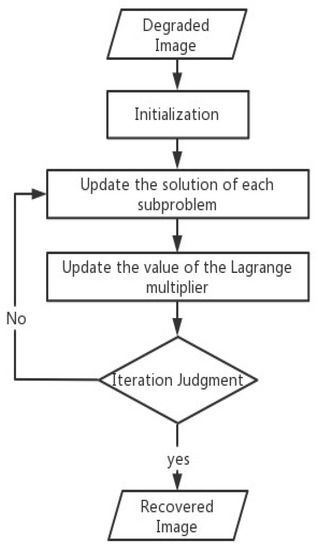
Figure 1. Flowchart of Algorithm 1.

In the following, we prove the convergence of Algorithm 1. The proof follows from the main idea of Theorem 1 of [30].

Algorithm 1 Proximal alternating direction method of multipliers (PADMM) for solving Problem (10).

Input: For arbitrary $u^0,v^0,z^0,x^0,y^0$, and $\beta ,\alpha ,{\rho }_1,{\rho }_2>0$.    1: update $u^{k+1}$ (via15);    2: update $v^{k+1}$ via (18);    3: update $z^{k+1}$ via (19);    4: update $x^{k+1}$ via (21) or (22);    5: update $y^{k+1}$ via (23);    6: Update the multipliers via     ${\xi }^{k+1}={\xi }^k+\gamma \beta (\nabla u^{k+1}-x^{k+1})$;     ${\zeta }^{k+1}={\zeta }^k+\gamma \alpha (K{u}^{k+1}-f-y^{k+1})$;     ${\pi }^{k+1}={\pi }^k+\gamma {\rho }_1(v^{k+1}\odot \omega \odot |y^{k+1}\left|\right)$;     ${\eta }^{k+1}={\eta }^k+\gamma {\rho }_2(u^{k+1}-z^{k+1})$;     Stops iteration when a given stopping criterion is reached. Output: $u^{k+1}$.

Theorem 1.

Let $X=(u,v,z,x,y)$, $Y=(\xi ,\zeta ,\pi ,\eta )$, $Z=(X,Y)$ and ${\left\{Z^k\right\}}_{k=1}^{\infty }$ be the sequence generated by Algorithm 1. If the sequence ${\left\{Y^k\right\}}_{k=1}^{\infty }$ is bounded and satisfies ${\displaystyle \sum _{k=0}^{\infty }}{\parallel Y^{k+1}-Y^k\parallel }^2<\infty$, then any accumulation point in the sequence is the KKT point of Problem (10).

Proof. 

According to the augmented Lagrangian function, the KKT condition at $\{u^{*},v^{*},z^{*},x^{*},y^{*},{\xi }^{*},{\zeta }^{*},{\pi }^{*},{\eta }^{*}\}$ can be derived:

$$\begin{array}{cc}\hfill & 0\in {\nabla }^T{\xi }^{*}+K^T{\zeta }^{*}+\partial {\delta }_C\left(u^{*}\right)+{\eta }^{*}\hfill \\ \hfill & 0\in {\pi }^{*}\odot \omega \odot \left|y^{*}\right|-1+\partial {\delta }_C\left(v^{*}\right)\hfill \\ \hfill & 0\in \partial \mu \parallel z^{*}{\parallel }_{*}-{\eta }^{*}\hfill \\ \hfill & 0\in \partial \lambda \parallel x^{*}{\parallel }_{p,1}-{\xi }^{*}\hfill \\ \hfill & 0\in {\pi }^{*}\odot v^{*}\odot \omega \odot \partial {\parallel y^{*}\parallel }_1-{\zeta }^{*}\hfill \\ \hfill & 0=\nabla u^{*}-x^{*}\hfill \\ \hfill & 0=K{u}^{*}-f-y^{*}\hfill \\ \hfill & 0=\omega \odot v^{*}\odot \left|y^{*}\right|\hfill \\ \hfill & 0=u^{*}-z^{*}.\hfill \end{array}$$

(24)

First, let us prove that ${\left\{Z^k\right\}}_{k=1}^{\infty }$ converges, that is, when $k\to \infty$, we have $Z^{k+1}-Z^k\to 0$. Its augmented Lagrange function can be written as

$$\begin{array}{cc}\hfill L\left(Z\right)=& ⟨1,1-v⟩+{\lambda \parallel x\parallel }_{p,1}+{\mu \parallel z\parallel }_{*}+\frac{\beta }{2}\parallel \nabla u-x+\frac{\xi }{\beta }{\parallel }^2-\frac{1}{2\beta }{\parallel \xi \parallel }^2\hfill \\ \hfill & +\frac{\alpha }{2}\parallel Ku-f-y+\frac{\zeta }{\alpha }{\parallel }^2-\frac{1}{2\alpha }{\parallel \zeta \parallel }^2+\frac{{\rho }_1}{2}\parallel v\odot \omega \odot \left|y\right|+\frac{\pi }{{\rho }_1}{\parallel }^2\hfill \\ \hfill & -\frac{1}{2{\rho }_1}{\parallel \pi \parallel }^2+\frac{{\rho }_2}{2}\parallel u-z+\frac{\eta }{{\rho }_2}{\parallel }^2-\frac{1}{2{\rho }_2}{\parallel \eta \parallel }^2.\hfill \end{array}$$

(25)

Since ${\left\{Y^k\right\}}_{k=1}^{\infty }$ is bounded, then $L\left(Z^k\right)$ is bounded. Let

$$\begin{array}{c}\hfill J\left(Z\right)=L\left(Z\right)+\frac{1}{2}\parallel u-u^{{}^{\prime }}{\parallel }_M^2+\frac{1}{2}{\parallel v-v^{{}^{\prime }}\parallel }_N^2,\end{array}$$

(26)

where $u^{{}^{\prime }},v^{{}^{\prime }}$ is the value of the previous iteration. $J\left(Z\right)$ is strongly convex with respect to u and v. Therefore, the second-order growth condition is satisfied for u and v, that is, there is $h>0$ such that

$$\begin{array}{c}\hfill J(u^k,v^k,z^k,x^k,y^k,Y^k)-J(u^{k+1},v^{k+1},z^k,x^k,y^k,Y^k)\ge \frac{h}{2}\parallel u^k-u^{k+1}{\parallel }_M^2+\frac{h}{2}{\parallel v^k-v^{k+1}\parallel }_N^2,\end{array}$$

(27)

and similarly for $z,x,y$, there is also a second-order growth condition, that is, the existence of $l>0$ such that

$$\begin{array}{cc}\hfill & J(u^{k+1},v^{k+1},z^k,x^k,y^k,Y^k)-J(u^{k+1},v^{k+1},z^{k+1},x^{k+1},y^{k+1},Y^k)\hfill \\ \hfill & \ge \frac{l}{2}\parallel x^k-x^{k+1}{\parallel }^2+\frac{l}{2}\parallel y^k-y^{k+1}{\parallel }^2+\frac{l}{2}{\parallel z^k-z^{k+1}\parallel }^2.\hfill \end{array}$$

(28)

Let $\rho =\frac{1}{2}min(h,l)$, and combine (27) with (28), we obtain

$$\begin{array}{c}\hfill J(X^k,Y^k)-J(X^{k+1},Y^k)\ge \rho {\parallel X^k-X^{k+1}\parallel }^2.\end{array}$$

(29)

On the other hand, according to the renewal principle of Lagrange multipliers.

$$\begin{array}{cc}\hfill & {\xi }^{k+1}={\xi }^k+\gamma \beta (\nabla u^{k+1}-x^{k+1})\hfill \\ \hfill & {\zeta }^{k+1}={\zeta }^k+\gamma \alpha (K{u}^{k+1}-f-y^{k+1})\hfill \\ \hfill & {\pi }^{k+1}={\pi }^k+\gamma {\rho }_1(v^{k+1}\odot \omega \odot |y^{k+1}\left|\right)\hfill \\ \hfill & {\eta }^{k+1}={\eta }^k+\gamma {\rho }_2(u^{k+1}-z^{k+1}).\hfill \end{array}$$

(30)

Let $p=min({\rho }_1,{\rho }_2,\alpha ,\beta )$, we have

$$\begin{array}{cc}\hfill J(X^{k+1},Y^{k+1})-J(X^{k+1},Y^k)& =⟨\nabla u^{k+1}-x^{k+1},{\xi }^{k+1}-{\xi }^k⟩+⟨K{u}^{k+1}-f-y^{k+1},{\zeta }^{k+1}-{\zeta }^k⟩\hfill \\ \hfill & +⟨v^{k+1}\odot \omega \odot |y^{k+1}|,{\pi }^{k+1}-{\pi }^k⟩+⟨u^{k+1}-z^{k+1},{\eta }^{k+1}-{\eta }^k⟩\hfill \\ \hfill & \le \frac{1}{\gamma p}{\parallel Y^{k+1}-Y^k\parallel }^2.\hfill \end{array}$$

(31)

Combining (29) and (31), we have

$$\begin{array}{c}\hfill J(X^k,Y^k)-J(X^{k+1},Y^{k+1})\ge \rho \parallel X^k-X^{k+1}{\parallel }^2+\frac{1}{\gamma p}{\parallel Y^{k+1}-Y^k\parallel }^2.\end{array}$$

(32)

Therefore,

$$\begin{array}{c}\hfill \sum _{k=0}^{\infty }(\rho \parallel X^k-X^{k+1}{\parallel }^2-\frac{1}{\gamma p}\parallel Y^{k+1}-Y^k{\parallel }^2)\le J(X^0,Y^0)-J(X^{\infty },Y^{\infty })<\infty .\end{array}$$

(33)

As a result, ${\displaystyle \sum _{k=0}^{\infty }}{\parallel Y^{k+1}-Y^k\parallel }^2<\infty$, i.e., $\underset{k\to \infty }{\lim }{\parallel Y^{k+1}-Y^k\parallel }^2=0$, which implies $\underset{k\to \infty }{\lim }{\parallel X^{k+1}-X^k\parallel }^2=0$ and $X^{k+1}-X^k\to 0(k\to \infty )$ hold. For $J\left(Z\right)$, its KKT conditions at $X^{k+1}$ are

$$\begin{array}{cc}\hfill & 0={\nabla }^T{\xi }^k+K^T{\zeta }^k+\partial {\delta }_C\left(u^{k+1}\right)+{\eta }^k+M(u^{k+1}-u^k)\hfill \\ \hfill & 0={\pi }^k\odot \omega \odot \left|y^{k+1}\right|-1+\partial {\delta }_C{v}^{k+1}+N(v^{k+1}-v^k)\hfill \\ \hfill & 0\in \partial \mu \parallel z^{k+1}{\parallel }_{\ast }-{\eta }^k\hfill \\ \hfill & 0\in \partial \lambda \parallel x^{k+1}{\parallel }_{p,1}-{\xi }^k\hfill \\ \hfill & 0\in {\pi }^k\odot v^{k+1}\odot \omega \odot {\parallel y^{k+1}\parallel }_1-{\zeta }^k.\hfill \end{array}$$

(34)

Combining $Z^{k+1}-Z^k\to 0$, we obtain

$$\begin{array}{cc}\hfill & 0={\nabla }^T{\xi }^{k+1}+K^T{\zeta }^{k+1}+\partial {\delta }_C\left(u^{k+1}\right)+{\eta }^{k+1}\hfill \\ \hfill & 0={\pi }^{k+1}\odot \omega \odot \left|y^{k+1}\right|-1+\partial {\delta }_C\left(v^{k+1}\right)\hfill \\ \hfill & 0\in \partial \mu \parallel z^{k+1}{\parallel }_{\ast }-{\eta }^{k+1}\hfill \\ \hfill & 0\in \partial \lambda \parallel x^{k+1}{\parallel }_{p,1}-{\xi }^{k+1}\hfill \\ \hfill & 0\in {\pi }^{k+1}\odot v^{k+1}\odot \omega \odot \partial {\parallel y^{k+1}\parallel }_1-{\zeta }^{k+1}\hfill \\ \hfill & 0=\nabla u^{k+1}-x^{k+1}\hfill \\ \hfill & 0=K{u}^{k+1}-f-y^{k+1}\hfill \\ \hfill & 0=\omega \odot v^{k+1}\odot \left|y^{k+1}\right|\hfill \\ \hfill & 0=u^{k+1}-z^{k+1}.\hfill \end{array}$$

(35)

which is the same as the KKT condition derived from Problem (10). Therefore, $Z^{k+1}$ is the KKT point of the problem. □

4. Numerical Experiments

In this section, the performance of the proposed method is verified by numerical experiments. The method is compared with ${\ell }_1$TV [29], ${\ell }_0$TV [30] and ${\ell }_0$OGSTV [32]. Here, ${\ell }_1$TV is used with the model with detection. All experiments were performed on 64-bit Windows 11 and MATLAB R2018b running on an Intel(R) Core(TM) i5-1035G1 CPU and 8 GB memory. We consider four test images of size $n\times m$ natural images: House ($512\times 512$), Mountain ($512\times 512$), Peppers ($512\times 512$), and Building ($517\times 493$), which are shown in Figure 2.

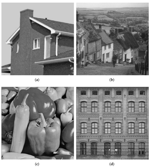
Figure 2. Test images. (a) House; (b) Mountain; (c) Peppers; (d) Building.

4.1. Experiment Setting

For natural image denoising, deblurring and low-rank image deblurring tests, we use the following method to generate simulation images.

(1) Natural image denoising. To generate noisy images, we add SP with noise levels of 10, 30, 50, 70 and 90% into the original image.

(2) Natural image deblurring. In order to generate noisy and blurred images, we use the following MATLAB function to generate a blurring kernel of radius $r=7$.

$$\begin{array}{cc}\hfill & [x,y]=meshgrid(-r:r,-r:r),\hfill \\ \hfill & K=double(x^2+y^2<=r^2),P=K/sum\left(K(:)\right).\hfill \end{array}$$

(36)

Then, noise levels of 10, 30, 50, 70 and 90% of the SP impulse noise are added.

(3) Low-rank image deblurring. To obtain noisy and blurred images of low rank, we used singular value division (SVD) to reduce the rank of the test image to 10, as shown in Figure 3. Then, the same method as described in (2) is performed on the images in Figure 3.

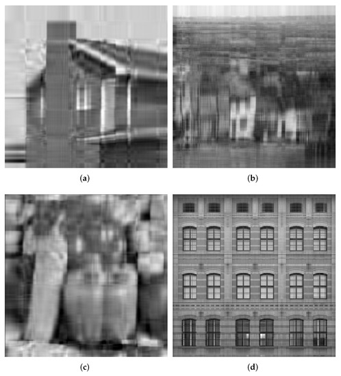
Figure 3. Low-rank images. (a) House; (b) Mountain; (c) Pepper; (d) Building.

In the numerical experiments, we set $\alpha =10$, $\beta =0.1$, ${\rho }_1=50$, and ${\rho }_2=1$ in the individual denoising and deblurring experiments. To obtain good results, we always adjust the regularization parameters $\lambda$ and $\mu$ in each test, where $\lambda \in \{0.1,0.3,0.5,0.7,0.9,1,2,3,\cdots 8\}$ and $\mu \in \{5,10,15,20,25,30,\cdots 200\}$. For the regularization parameter in ${\ell }_1\mathrm{TV}$, we sweep over$\{200,300,400,500,600,700,800\}$. For the regularization parameter in ${\ell }_0\mathrm{OGSTV}$, we sweep over$\{0.1,0.5,1,2,3,\cdots 10\}$. We use the same stopping criterion as [30], defined as $\parallel \nabla u^k-x^k{\parallel }_2\le \frac{1}{255}$ and $\parallel K{u}^k-f-y^k{\parallel }_2\le \frac{1}{255}$ and $\parallel \omega \odot v^k\odot |y^k{|\parallel }_2\le \frac{1}{255}$ and $\parallel u^k-z^k{\parallel }_2\le \frac{1}{255}$. ${\ell }_1$TV, ${\ell }_0$TV and ${\ell }_0$OGSTV also adopt a similar stopping criterion.

To evaluate the effectiveness of these models in recovering images, we use the peak signal-to-noise ratio (PSNR), and the structural similarity ratio (SSIM ) index, defined as follows:

$$\begin{array}{c}\hfill PSNR=10lo{g}_{10}\frac{P^2}{\frac{1}{mn}\sum _{i,j}(u_{i,j}-{\tilde{u}}_{i,j})},\end{array}$$

and

$$\begin{array}{c}\hfill SSIM=\frac{(2{\mu }_u{\mu }_{\tilde{u}}+c_1)(2{\sigma }_{u\tilde{u}}+c_2)}{(2{\mu }_u^2{\mu }_{\tilde{u}}^2+c_1)({\sigma }_u^2+{\sigma }_{\tilde{u}}^2+c_2)},\end{array}$$

where P is the maximum peak value of the original image u, $\tilde{u}$ is the restored image, $c_1>0$ and $c_2>0$ are small constants, ${\mu }_u$ and ${\mu }_{\tilde{u}}$ are the mean values of u and $\tilde{u}$, respectively, ${\sigma }_u$ and ${\sigma }_{\tilde{u}}$ are the variances of u and $\tilde{u}$, and ${\sigma }_{u\tilde{u}}$ is the covariance of u and $\tilde{u}$.

4.2. Natural Images Denoising

In this subsection, we compare the performance of our model with ${\ell }_0$TV, ${\ell }_1$TV, and ${\ell }_0$OGSTV for pure denoising. Table 1 shows the results of the different recovery methods. As can be seen from the table, in most cases, the proposed model outperforms ${\ell }_0$TV and ${\ell }_1$TV. This is because the combination of ${\ell }_0$ TV and nuclear norm can better handle the texture and edge information in the image while removing noise, whereas the ${\ell }_0$ TV and ${\ell }_1$ TV methods may encounter difficulties in dealing with the texture and edge information, resulting in artefacts and blurring. In particular, for Building images with low-rank structures, Our proposed model also outperforms ${\ell }_0$OGSTV in PSNR values, and is 1–2 dB and 3–4 dB higher than ${\ell }_0$TV and ${\ell }_1$TV, respectively, mainly because we include the nuclear norm as a penalty term. However, for the House and Mountain images, the ${\ell }_0$OGSTV model outperforms the proposed model. Figure 4 and Figure 5 show a visual comparison of the different methods for recovering the damaged Building and Pepper images at different noise levels. It can be observed that the proposed model recovered the images better than the other models. Specifically, for high SP noise, the proposed model retains the neat edges better, which can be seen more visually from the local images. In addition, Figure 6 demonstrates the variation of PSNR over time for different methods to recover the Pepper images with different noise levels. It shows that our proposed method takes approximately the same amount of time to denoise at different noise levels, while ${\ell }_1$TV and ${\ell }_0$OGSTV take longer when the noise level is very high.

Table 1. The PSNR (dB), SSIM, and number of iterations (Iter) of different methods for images corrupted by SP noise. The bold data represents the best PSNR, SSIM, and the least number of iterations, respectively.

Image	Noise Levels	Input PSNR/SSIM	${\mathit{\ell }}_1$TV	${\mathit{\ell }}_0$TV	${\mathit{\ell }}_0$OGSTV	Ours
House	$10\%$	$15.23/0.13$	$54.88/0.9988/293$	$55.23/0.9989/\mathbf{123}$	$58.06/0.9994/196$	$\mathbf{60}.\mathbf{18}/\mathbf{0}.\mathbf{9996}/274$
	$30\%$	$10.44/0.03$	$47.70/0.9946/430$	$48.04/0.9950/\mathbf{181}$	$\mathbf{50}.\mathbf{84}/\mathbf{0}.\mathbf{9970}/217$	$50.14/0.9968/222$
	$50\%$	$8.20/0.01$	$42.62/0.9852/626$	$42.91/0.9859/243$	$\mathbf{45}.\mathbf{77}/\mathbf{0}.\mathbf{9916}/\mathbf{226}$	$43.70/0.9882/245$
	$70\%$	$6.73/0.009$	$36.69/0.9579/962$	$37.12/0.9600/\mathbf{224}$	$\mathbf{39}.\mathbf{95}/\mathbf{0}.\mathbf{9757}/228$	$37.38/0.9626/305$
	$90\%$	$5.64/0.005$	$28.57/0.8703/2418$	$28.79/0.8719/\mathbf{241}$	$\mathbf{31}.\mathbf{77}/\mathbf{0}.\mathbf{9108}/264$	$28.79/0.8724/247$
Mountain	$10\%$	$15.34/0.20$	$41.11/0.9864/249$	$41.17/0.9866/117$	$\mathbf{42}.\mathbf{30}/\mathbf{0}.\mathbf{9888}/116$	$41.54/0.9872/\mathbf{110}$
	$30\%$	$10.59/0.05$	$35.62/0.9522/412$	$35.65/0.9529/176$	$\mathbf{36.71}/\mathbf{0.9601}/\mathbf{130}$	$35.93/0.9546/152$
	$50\%$	$8.37/0.02$	$32.32/0.9010/608$	$32.38/0.9023/187$	$\mathbf{33}.\mathbf{42}/\mathbf{0}.\mathbf{9175}/\mathbf{144}$	$32.63/0.9055/169$
	$70\%$	$6.89/0.01$	$29.21/0.8129/776$	$29.34/0.8162/188$	$\mathbf{30}.\mathbf{37}/\mathbf{0}.\mathbf{8452}/\mathbf{183}$	$29.50/0.8205/195$
	$90\%$	$5.80/0.006$	$25.05/0.6268/1376$	$25.37/0.6340/\mathbf{198}$	$\mathbf{26}.\mathbf{54}/\mathbf{0}.\mathbf{6876}/230$	$25.38/0.6352/220$
Pepper	$10\%$	$15.28/0.16$	$44.55/0.9961/430$	$44.63/0.9962/\mathbf{193}$	$46.22/0.9972/201$	$\mathbf{58}.\mathbf{51}/\mathbf{0}.\mathbf{9997}/299$
	$30\%$	$10.55/0.04$	$39.22/0.9864/524$	$39.36/0.9868/211$	$40.09/0.9887/210$	$\mathbf{44}.\mathbf{83}/\mathbf{0}.\mathbf{9948}/\mathbf{198}$
	$50\%$	$8.32/0.02$	$35.76/0.9696/621$	$35.99/0.9709/212$	$36.27/0.9367/\mathbf{211}$	$\mathbf{37}.\mathbf{98}/\mathbf{0}.\mathbf{9794}/222$
	$70\%$	$6.84/0.01$	$32.28/0.9364/820$	$32.37/0.9380/218$	$32.90/0.9454/\mathbf{215}$	$\mathbf{32}.\mathbf{97}/\mathbf{0}.\mathbf{9439}/243$
	$90\%$	$5.75/0.005$	$26.33/0.8382/1384$	$26.53/0.8371/\mathbf{209}$	$\mathbf{28}.\mathbf{00}/\mathbf{0}.\mathbf{8709}/227$	$26.50/0.8372/235$
Building	$10\%$	$15.59/0.36$	$35.67/0.9826/194$	$35.68/0.9826/134$	$38.67/0.9896/\mathbf{116}$	$\mathbf{39}.\mathbf{89}/\mathbf{0}.\mathbf{9906}/161$
	$30\%$	$10.84/0.13$	$29.86/0.9314/238$	$29.86/0.9316/178$	$32.18/0.9547/\mathbf{126}$	$\mathbf{33}.\mathbf{85}/\mathbf{0}.\mathbf{9600}/182$
	$50\%$	$8.62/0.06$	$26.55/0.8513/292$	$26.54/0.8515/189$	$28.13/0.8888/\mathbf{129}$	$\mathbf{30}.\mathbf{21}/\mathbf{0}.\mathbf{9147}/181$
	$70\%$	$7.15/0.03$	$23.76/0.7160/366$	$23.79/0.7165/188$	$24.78/0.7642/\mathbf{131}$	$\mathbf{26}.\mathbf{91}/\mathbf{0}.\mathbf{8284}/183$
	$90\%$	$6.06/0.01$	$20.02/0.4288/677$	$20.31/0.4347/195$	$21.24/0.5098/\mathbf{140}$	$\mathbf{22}.\mathbf{83}/\mathbf{0}.\mathbf{6365}/201$

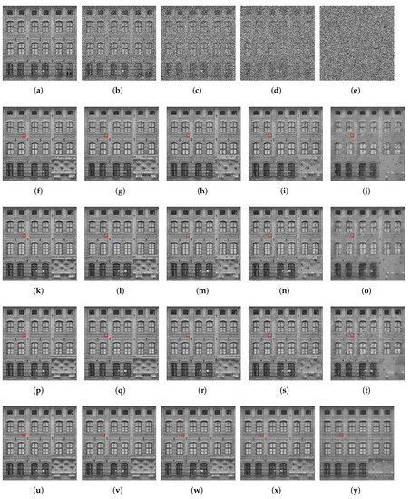
Figure 4. Comparison of restored images from different methods for the images degraded by SP noise. First line: corrupted images. Second line: restored images by ${\ell }_1$TV. Third line:restored images by ${\ell }_0$TV. Forth line: restored images by ${\ell }_0$OGSTV. Fifth line: restored images by Ours. (a) $10\%,15.59$; (b) $30\%,10.84$; (c) $50\%,8.62$; (d) $70\%,7.15$; (e) $90\%,6.06$; (f) $10\%,35.67$; (g) $30\%,29.86$; (h) $50\%,26.55$; (i) $70\%,23.76$; (j) $90\%,20.02$; (k) $10\%,35.68$; (l) $30\%,29.86$; (m) $50\%,26.54$; (n) $70\%,23.79$; (o) $90\%,20.31$; (p) $10\%,38.67$; (q) $30\%,32.18$; (r) $50\%,28.13$; (s) $70\%,24.78$; (t) $90\%,21.24$; (u) $10\%,39.89$; (v) $30\%,33.85$; (w) $50\%,30.21$; (x) $70\%,26.91$; (y) $90\%,22.83$. The numbers represent the noise level and PSNR (dB) of the image.

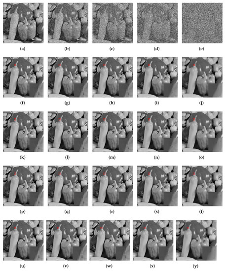
Figure 5. Comparison of restored images from different methods for the images degraded by SP noise. First line: corrupted images. Second line: restored images by ${\ell }_1$TV. Third line:restored images by ${\ell }_0$TV. Forth line: restored images by ${\ell }_0$OGSTV. Fifth line: restored images by Ours. (a) $10\%,15.28$; (b) $30\%,10.55$; (c) $50\%,8.32$; (d) $70\%,6.84$; (e) $90\%,5.75$; (f) $10\%,44.55$; (g) $30\%,39.22$; (h) $50\%,35.76$; (i) $70\%,32.28$; (j) $90\%,26.33$; (k) $10\%,44.63$; (l) $30\%,39.36$; (m) $50\%,35.99$; (n) $70\%,32.37$; (o) $90\%,26.53$; (p) $10\%,46.22$; (q) $30\%,40.09$; (r) $50\%,36.27$; (s) $70\%,32.90$; (t) $90\%,28.00$; (u) $10\%,58.51$; (v) $30\%,44.83$; (w) $50\%,37.98$; (x) $70\%,32.97$; (y) $90\%,26.50$. The numbers represent the noise level and PSNR (dB) of the image.

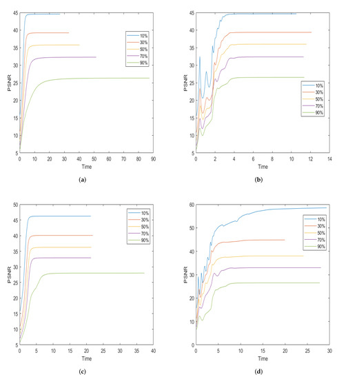
Figure 6. The PSNR values with respect to the CPU time in seconds are compared for the test image of Peppers among the different methods. (a) ${\ell }_1$TV; (b) ${\ell }_0$TV; (c) ${\ell }_0$OGSTV; (d) Ours.

4.3. Natural Images Deblurring

In this subsection, we compare the performance of our model with ${\ell }_0$TV, ${\ell }_1$TV, and ${\ell }_0$OGSTV for deblurring with SP noise. Table 2 shows the recovery results of the different methods. In most situations, the proposed model outperforms ${\ell }_0$TV and ${\ell }_1$TV in terms of PSNR and SSIM. For images of House and Mountain, the ${\ell }_0$OGSTV model outperforms the proposed model. This is attributed to ${\ell }_0$OGSTV using external norm, which can comprehensively consider the structural information of the image, thereby achieving a better deblurring effect. However, for Building images with low-rank structures, the proposed model also outperforms ${\ell }_0$OGST. This phenomenon indicates that our method performs well in deblurring low-rank images or images with low-rank structures. Figure 7 and Figure 8 show a visual comparison of the different methods for recovering the Building and Pepper images with blurring and different noise levels. It can be observed that the model proposed in this paper is better than other methods in terms of PSNR and visual quality, retaining clear edges and sharper images, especially at higher levels of noise. In addition, Figure 9 shows the variation in PSNR over time for different methods to recover the House image at different noise levels. Figure 9 shows that the ${\ell }_0$TV method requires the least time for image deblurring, while the time for deblurring using ${\ell }_1$TV and our method decreases as the noise level increases. In contrast, the ${\ell }_0$OGSTV method takes longer for deblurring, especially when the noise level reaches 90%, since inner and outer iterations need to be solved when using the ${\ell }_0$OGSTV method for deblurring, which requires more time.

Table 2. The PSNR (dB), SSIM, and number of iterations (Iter) of different methods for images corrupted by blurring with SP noise. The bold data represents the best PSNR, SSIM, and the least number of iterations, respectively.

Image	Noise Levels	Input PSNR/SSIM	${\mathit{\ell }}_1$TV	${\mathit{\ell }}_0$TV	${\mathit{\ell }}_0$OGSTV	Ours
House	$10\%$	$14.90/0.08$	$58.03/0.9992/2882$	$53.94/0.9980/\mathbf{1204}$	$\mathbf{58}.\mathbf{27}/\mathbf{0}.\mathbf{9992}/1819$	$56.25/0.9987/1405$
	$30\%$	$10.35/0.02$	$51.75/0.9970/2653$	$49.68/0.9955/\mathbf{1167}$	$\mathbf{54}.\mathbf{66}/\mathbf{0}.\mathbf{9982}/1794$	$52.93/0.9974/1419$
	$50\%$	$8.16/0.01$	$46.95/0.9923/2218$	$45.75/0.9905/\mathbf{1203}$	$\mathbf{50}.\mathbf{96}/\mathbf{0}.\mathbf{9960}/1648$	$49.18/0.9943/1470$
	$70\%$	$6.71/0.006$	$42.24/0.9812/1936$	$41.60/0.9794/\mathbf{1234}$	$\mathbf{46}.\mathbf{47}/\mathbf{0}.\mathbf{9899}/1413$	$44.80/0.9864/1378$
	$90\%$	$5.64/0.004$	$35.94/0.9382/1627$	$35.76/0.9387/\mathbf{788}$	$\mathbf{39}.\mathbf{11}/\mathbf{0}.\mathbf{9587}/5221$	$37.79/0.9508/1237$
Mountain	$10\%$	$14.86/0.07$	$41.46/0.9805/2581$	$40.96/0.9791/\mathbf{1682}$	$\mathbf{42}.\mathbf{96}/\mathbf{0}.\mathbf{9860}/4014$	$40.89/0.9788/1981$
	$30\%$	$10.46/0.01$	$37.47/0.9546/1864$	$37.14/0.9526/\mathbf{1393}$	$\mathbf{38}.\mathbf{38}/\mathbf{0}.\mathbf{9621}/2345$	$37.35/0.9542/1558$
	$50\%$	$8.32/0.009$	$34.53/0.9180/1346$	$34.35/0.9166/\mathbf{1268}$	$\mathbf{35}.\mathbf{39}/\mathbf{0}.\mathbf{9297}/1512$	$34.60/0.9193/1387$
	$70\%$	$6.87/0.006$	$31.84/0.8603/\mathbf{1041}$	$31.77/0.8599/1088$	$\mathbf{32}.\mathbf{63}/\mathbf{0}.\mathbf{8781}/1131$	$32.03/0.8649/1296$
	$90\%$	$5.80/0.004$	$28.45/0.7340/866$	$28.49/0.7369/\mathbf{814}$	$28.52/0.7494/8431$	$\mathbf{28}.\mathbf{76}/\mathbf{0}.\mathbf{7479}/1176$
Pepper	$10\%$	$14.87/0.09$	$\mathbf{63}.\mathbf{72}/\mathbf{0}.\mathbf{9998}/2745$	$53.71/0.9981/\mathbf{1260}$	$51.64/0.9969/2970$	$56.04/0.9988/1450$
	$30\%$	$10.43/0.02$	$\mathbf{51}.\mathbf{79}/\mathbf{0}.\mathbf{9972}/2651$	$47.58/0.9938/\mathbf{1172}$	$46.42/0.9922/2482$	$49.98/0.9959/1386$
	$50\%$	$8.27/0.01$	$43.94/0.9877/1876$	$41.92/0.9829/\mathbf{1218}$	$41.70/0.9826/1864$	$\mathbf{44}.\mathbf{09}/\mathbf{0}.\mathbf{9877}/1470$
	$70\%$	$6.82/0.006$	$37.83/0.9647/1331$	$37.02/0.9607/\mathbf{997}$	$37.32/0.9642/1387$	$\mathbf{38}.\mathbf{49}/\mathbf{0}.\mathbf{9674}/1166$
	$90\%$	$5.75/0.004$	$31.97/0.9026/938$	$31.83/0.9027/\mathbf{784}$	$32.13/0.9134/8879$	$\mathbf{32}.\mathbf{54}/\mathbf{0}.\mathbf{9116}/1132$
Building	$10\%$	$14.31/0.06$	$\mathbf{37}.\mathbf{92}/\mathbf{0}.\mathbf{9795}/1795$	$36.66/0.9739/\mathbf{1652}$	$36.89/0.9744/3006$	$37.61/0.9781/1891$
	$30\%$	$10.46/0.02$	$33.13/0.9447/\mathbf{1163}$	$32.46/0.9373/1655$	$33.08/0.9440/1760$	$\mathbf{34}.\mathbf{11}/\mathbf{0}.\mathbf{9529}/1636$
	$50\%$	$8.46/0.01$	$29.44/0.8843/\mathbf{760}$	$29.17/0.8793/1130$	$29.29/0.8822/1392$	$\mathbf{31}.\mathbf{22}/\mathbf{0}.\mathbf{9129}/1477$
	$70\%$	$7.08/0.007$	$26.19/0.7793/\mathbf{527}$	$26.13/0.7785/901$	$27.41/0.8052/656$	$\mathbf{28}.\mathbf{40}/\mathbf{0}.\mathbf{8451}/1199$
	$90\%$	$6.04/0.003$	$22.74/0.5662/\mathbf{429}$	$22.75/0.5666/825$	$22.95/0.5833/1243$	$\mathbf{24}.\mathbf{67}/\mathbf{0}.\mathbf{6810}/1203$

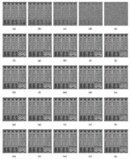
Figure 7. Comparison of restored images from different methods for the images degraded by SP noise and blur kernel. First line: corrupted images. Second line: restored images by ${\ell }_1$TV. Third line:restored images by ${\ell }_0$TV. Forth line: restored images by ${\ell }_0$OGSTV. Fifth line: restored images by Ours. (a) $10\%,14.31$; (b) $30\%,10.46$; (c) $50\%,8.46$; (d) $70\%,7.08$; (e) $90\%,6.04$; (f) $10\%,37.92$; (g) $30\%,33.13$; (h) $50\%,29.44$; (i) $70\%,26.19$; (j) $90\%,22.74$; (k) $10\%,36.66$; (l) $30\%,32.46$; (m) $50\%,29.17$; (n) $70\%,26.13$; (o) $90\%,22.75$; (p) $10\%,36.89$; (q) $30\%,33.08$; (r) $50\%,29.29$; (s) $70\%,27.41$; (t) $90\%,22.95$; (u) $10\%,37.61$; (v) $30\%,34.11$; (w) $50\%,31.22$; (x) $70\%,28.40$; (y) $90\%,24.67$. The numbers represent the noise level and PSNR (dB) of the image.

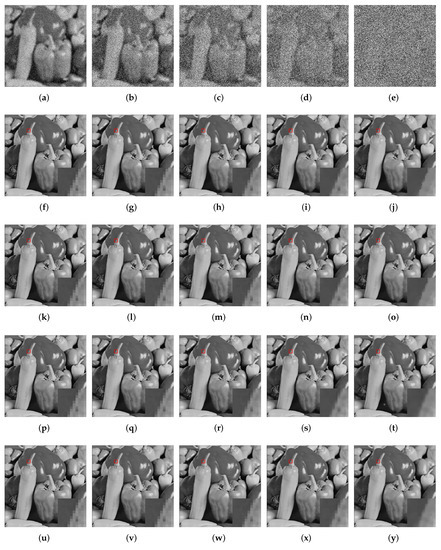
Figure 8. Comparison of restored images from different methods for the images degraded by SP noise and blur kernel. First line: corrupted images. Second line: restored images by ${\ell }_1$TV. Third line:restored images by ${\ell }_0$TV. Forth line: restored images by ${\ell }_0$OGSTV. Fifth line: restored images by Ours. (a) $10\%,14.87$; (b) $30\%,10.43$; (c) $50\%,8.27$; (d) $70\%,6.82$; (e) $90\%,5.75$; (f) $10\%,63.72$; (g) $30\%,51.79$; (h) $50\%,43.94$; (i) $70\%,37.83$; (j) $90\%,31.97$; (k) $10\%,53.71$; (l) $30\%,47.58$; (m) $50\%,41.92$; (n) $70\%,37.02$; (o) $90\%,31.83$; (p) $10\%,51.64$; (q) $30\%,46.42$; (r) $50\%,41.70$; (s) $70\%,37.32$; (t) $90\%,32.13$; (u) $10\%,56.04$; (v) $30\%,49.98$; (w) $50\%,44.09$; (x) $70\%,38.49$; (y) $90\%,32.54$. The numbers represent the noise level and PSNR (dB) of the image.

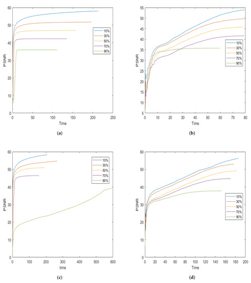
Figure 9. The PSNR values with respect to the CPU time in seconds are compared for the test image of House among the different methods. (a) ${\ell }_1$TV; (b) ${\ell }_0$TV; (c) ${\ell }_0$OGSTV; (d) Ours.

4.4. Low-Rank Image Deblurring

In this subsection, we compare the performance of our model with ${\ell }_0$TV, ${\ell }_1$TV and ${\ell }_0$OGSTV for deblurring low-rank images. Table 3 presents the recovery results of the different methods. From Table 3, it is evident that our model outperforms the other three methods in most situations. Low-rank images usually contain the main structural information of an image, and the nuclear norm as a low-rank constraint can better recover global structural information, thereby improving the deblurring effect, which is consistent with the theoretical studies. Moreover, as the level of noise increases, the difference in PSNR between our model and the other three methods becomes more significant, further demonstrating the higher stability of our approach in dealing with low-rank image tasks. However, for Pepper images, ${\ell }_1$TV outperforms our model at noise level of 10 and 30%. Overall, our method performs well in processing low-rank images. Figure 10 visually compares the different methods for recovering low-rank Building images under blurring and various noise levels. As shown in Figure 10, our model can achieve better visualization for low-rank image recovery compared to other methods.

Table 3. The PSNR(dB), SSIM, and number of iterations (Iter) of different methods for images corrupted by blurring with SP noise. The bold data represents the best PSNR, SSIM, and the least number of iterations, respectively.

Image	Noise Levels	Input PSNR/SSIM	${\mathit{\ell }}_1$TV	${\mathit{\ell }}_0$TV	${\mathit{\ell }}_0$OGSTV	Ours
House	$10\%$	$15.13/0.08$	$62.47/0.9997/2135$	$55.21/0.9987/1689$	$59.84/0.9994/\mathbf{1572}$	$\mathbf{63}.\mathbf{50}/\mathbf{0}.\mathbf{9998}/1771$
	$30\%$	$10.46/0.02$	$57.49/0.9991/2224$	$52.48/0.9976/\mathbf{1618}$	$58.48/0.9992/3675$	$\mathbf{63}.\mathbf{31}/\mathbf{0}.\mathbf{9998}/1770$
	$50\%$	$8.24/0.01$	$52.64/0.9975/2084$	$49.47/0.9954/\mathbf{1680}$	$56.72/0.9989/4116$	$\mathbf{63}.\mathbf{20}/\mathbf{0}.\mathbf{9998}/1775$
	$70\%$	$6.78/0.006$	$47.54/0.9930/1758$	$45.60/0.9899/\mathbf{1588}$	$52.99/0.976/4304$	$\mathbf{59}.\mathbf{37}/\mathbf{0}.\mathbf{9995}/1860$
	$90\%$	$5.70/0.004$	$40.38/0.9719/\mathbf{1292}$	$39.14/0.9656/1393$	$44.00/0.9886/9119$	$\mathbf{52}.\mathbf{72}/\mathbf{0}.\mathbf{9978}/1830$
Mountain	$10\%$	$15.21/0.07$	$51.90/0.9968/4876$	$48.79/0.9939/1143$	$51.49/0.9963/3519$	$\mathbf{57}.\mathbf{81}/\mathbf{0}.\mathbf{9993}/\mathbf{1130}$
	$30\%$	$10.60/0.01$	$46.49/0.9898/3412$	$45.04/0.9863/\mathbf{983}$	$48.57/0.9931/4239$	$\mathbf{56}.\mathbf{98}/\mathbf{0}.\mathbf{9991}/1203$
	$50\%$	$8.41/0.008$	$42.63/0.9771/2370$	$41.81/0.9734/\mathbf{904}$	$45.11/0.9858/4338$	$\mathbf{55}.\mathbf{80}/\mathbf{0}.\mathbf{9989}/1292$
	$70\%$	$6.94/0.005$	$39.07/0.9524/1754$	$38.63/0.9490/\mathbf{829}$	$41.20/0.9683/4352$	$\mathbf{52}.\mathbf{27}/\mathbf{0}.\mathbf{9975}/1295$
	$90\%$	$5.86/0.003$	$34.68/0.8860/1460$	$34.64/0.8873/\mathbf{750}$	$36.04/0.9125/10106$	$\mathbf{43}.\mathbf{93}/\mathbf{0}.\mathbf{9845}/1292$
Pepper	$10\%$	$15.26/0.09$	$\mathbf{68}.\mathbf{88}/\mathbf{0}.\mathbf{9999}/2482$	$48.49/0.9949/\mathbf{1144}$	$55.45/0.9985/2319$	$52.09/0.9970/1620$
	$30\%$	$10.63/0.02$	$\mathbf{57}.\mathbf{65}/\mathbf{0}.\mathbf{9991}/2693$	$46.97/0.9923/\mathbf{1140}$	$51.19/0.9964/2222$	$51.64/0.9968/1598$
	$50\%$	$8.40/0.01$	$48.95/0.9943/1884$	$44.05/0.9850/\mathbf{866}$	$47.00/0.9916/1874$	$\mathbf{50}.\mathbf{46}/\mathbf{0}.\mathbf{9964}/1620$
	$70\%$	$6.93/0.006$	$42.98/0.9805/1158$	$38.61/0.9673/\mathbf{729}$	$42.82/0.9813/1441$	$\mathbf{47}.\mathbf{78}/\mathbf{0}.\mathbf{9942}/1586$
	$90\%$	$5.85/0.004$	$36.59/0.9365/684$	$36.23/0.9344/\mathbf{574}$	$37.79/0.9538/8233$	$\mathbf{41}.\mathbf{32}/\mathbf{0}.\mathbf{9806}/1530$
Building	$10\%$	$14.64/0.07$	$43.80/0.9919/5000$	$39.66/0.9815/\mathbf{1681}$	$45.96/0.9946/4041$	$\mathbf{46}.\mathbf{86}/\mathbf{0}.\mathbf{9964}/2041$
	$30\%$	$10.60/0.02$	$37.04/0.9685/2406$	$35.46/0.9573/\mathbf{1506}$	$40.86/0.9849/4433$	$\mathbf{44}.\mathbf{99}/\mathbf{0}.\mathbf{9945}/1714$
	$50\%$	$8.55/0.01$	$32.54/0.9243/1379$	$31.89/0.9152/\mathbf{1210}$	$35.78/0.9588/4658$	$\mathbf{43}.\mathbf{62}/\mathbf{0}.\mathbf{9927}/1680$
	$70\%$	$7.14/0.007$	$28.77/0.8442/\mathbf{996}$	$28.56/0.8389/1042$	$30.60/0.8885/1823$	$\mathbf{41}.\mathbf{29}/\mathbf{0}.\mathbf{9982}/1530$
	$90\%$	$6.10/0.004$	$24.75/0.6687/952$	$24.67/0.6622/\mathbf{813}$	$25.21/0.6952/4962$	$\mathbf{32}.\mathbf{32}/\mathbf{0}.\mathbf{9242}/1215$

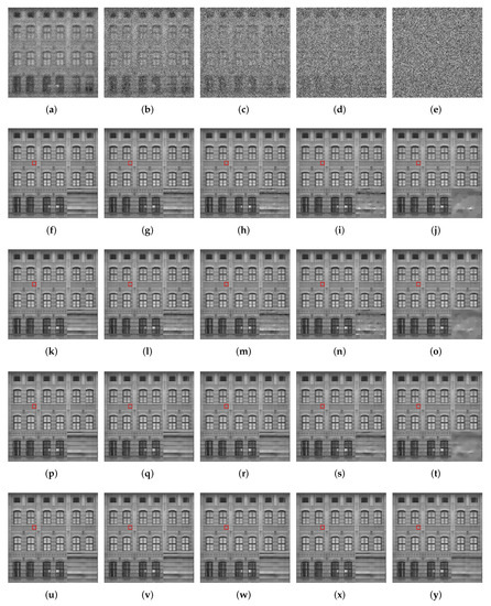
Figure 10. Comparison of restored images from different methods for the images degraded by SP noise and blur kernel. First line: corrupted images. Second line: restored images by ${\ell }_1$TV. Third line:restored images by ${\ell }_0$TV. Forth line: restored images by ${\ell }_0$OGSTV. Fifth line: restored images by Ours. (a) $10\%,14.64$; (b) $30\%,10.60$; (c) $50\%,8.55$; (d) $70\%,7.14$; (e) $90\%,6.10$; (f) $10\%,43.80$; (g) $30\%,37.04$; (h) $50\%,32.54$; (i) $70\%,28.77$; (j) $90\%,24.75$; (k) $10\%,39.66$; (l) $30\%,35.46$; (m) $50\%,31.89$; (n) $70\%,28.56$; (o) $90\%,24.67$; (p) $10\%,45.96$; (q) $30\%,40.86$; (r) $50\%,35.78$; (s) $70\%,30.60$; (t) $90\%,25.21$; (u) $10\%,46.86$; (v) $30\%,44.99$; (w) $50\%,43.62$; (x) $70\%,41.29$; (y) $90\%,32.32$. The numbers represent the noise level and PSNR (dB) of the image.

4.5. Real Image Denoising

In this section, we verify the effectiveness of our method on real images by selecting an image that has been corrupted by impulse noise, as shown in Figure 11. The figure illustrates the real image and the images restored by using four different methods. It can be seen that our method exhibits good performance on real images. The image is obtained from https://www.usgs.gov/landsat-missions/impulse-noise, accessed on 24 May 2023.

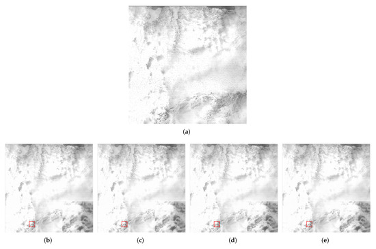
Figure 11. Comparison of restored images by using different methods for a real image with impulse noise. (a) real image with impulse noise. (b) restored image by ${\ell }_1$TV. (c) restored image by ${\ell }_0$TV. (d) restored image by ${\ell }_0$OGSTV. (e) restored image by Ours.

5. Conclusions

In this paper, we proposed a novel model that utilizes a combination of ${\ell }_0$TV and nuclear norm to remove impulse noise. Despite the challenge of dealing with a non-convex and non-smooth problem, we developed a solution through mathematical program with equilibrium constraints (MPEC) and proximal ADMM. The convergence of our proposed algorithm was proven under certain conditions. The experimental results demonstrated that our model surpasses other state-of-the-art methods, such as ${\ell }_0$TV, ${\ell }_1$TV, and ${\ell }_0$OGSTV, in processing low-rank images, as seen through its higher PSNR and SSIM values. In this paper, the solution process involves calculating the proximity operator of the nuclear norm, which requires using the singular value decomposition of the matrix. As a result, the computation speed may decrease when dealing with large matrix dimensions. Therefore, it is necessary to make trade-offs based on specific application scenarios. In the future, we will combine weighted nuclear norm and data fidelity terms. Weighted nuclear norm assigns different weights to different image blocks, fully utilizing the correlation between features and the sparsity of the data, resulting in better image recovery performance.

References

- Lin, T.C. A new adaptive center weighted median filter for suppressing impulsive noise in images. Inf. Sci. 2007, 177, 1073–1087. [Google Scholar] [CrossRef]
- Zhang, P.X.; Li, F. A New Adaptive Weighted Mean Filter for Removing Salt-and-Pepper Noise. IEEE Signal Process. Lett. 2014, 21, 1280–1283. [Google Scholar] [CrossRef]
- Zhang, Z.; Han, D.; Dezert, J.; Yang, Y. A new adaptive switching median filter for impulse noise reduction with pre-detection based on evidential reasoning. Signal Process. 2018, 147, 173–189. [Google Scholar] [CrossRef]
- Zhang, W.H.; Jin, L.H.; Song, E.N.; Xu, X.Y. Removal of impulse noise in color images based on convolutional neural network. Appl. Soft Comput. 2019, 32, 105558. [Google Scholar] [CrossRef]
- Li, G.Y.; Xu, X.L.; Zhang, M.H.; Liu, Q.G. Densely connected network for impulse noise removal. Pattern Anal. Appl. 2020, 23, 1263–1275. [Google Scholar] [CrossRef]
- Zhang, K.; Zuo, W.M.; Chen, Y.J.; Meng, D.Y.; Zhang, L. Beyond a Gaussian Denoiser: Residual Learning of Deep CNN for Image Denoising. IEEE Trans. Image Process. 2017, 26, 3142–3155. [Google Scholar] [CrossRef] [PubMed]
- Zhang, K.; Zuo, W.M.; Zhang, L. FFDNet: Toward a Fast and Flexible Solution for CNN-Based Image Denoising. IEEE Trans. Image Process. 2018, 27, 4608–4622. [Google Scholar] [CrossRef]
- Guo, B.Y.; Song, K.C.; Dong, H.W.; Yan, Y.H.; Tu, Z.B.; Zhu, L. NERNet: Noise estimation and removal network for image denoising. J. Vis. Commun. Image Represent. 2020, 71, 102851. [Google Scholar] [CrossRef]
- Chan, T.F.; Esedoglu, S. Aspects of total variation regularized l1 function approximation. SIAM J. Appl. Math. 2005, 65, 1817–1837. [Google Scholar] [CrossRef]
- Yang, J.F.; Zhang, Y.; Yin, W.T. An efficient TVL1 algorithm for deblurring multichannel images corrupted by impulsive noise. SIAM J. Sci. Comput. 2009, 31, 2842–2865. [Google Scholar] [CrossRef]
- Guo, X.X.; Li, F.; Ng, M.K. A fast ℓ1-TV algorithm for image restoration. SIAM J. Sci. Comput. 2009, 31, 2322–2341. [Google Scholar] [CrossRef]
- Yuan, J.; Shi, J.; Tai, X.C. A convex and exact approach to discrete constrained TV-L1 image approximation. East Asian J. Appl. Math. 2011, 1, 172–186. [Google Scholar] [CrossRef]
- Micchelli, C.A.; Shen, L.X.; Xu, L.Y.S.; Zeng, X. Proximity algorithms for the L1/TV image denoising model. Adv. Comput. Math. 2013, 38, 401–426. [Google Scholar] [CrossRef]
- Liu, Q.G.; Xiong, B.; Yang, D.C.; Zhang, M.H. A generalized relative total variation method for image smoothing. Multimed. Tools Appl. 2016, 75, 7909–7930. [Google Scholar] [CrossRef]
- Shi, M.Z.; Han, T.T.; Liu, S.Q. Total variation image restoration using hyper-Laplacian prior with overlapping group sparsity. Signal Process. 2016, 126, 65–76. [Google Scholar] [CrossRef]
- Lanza, A.; Morigi, S.; Sgallari, F. A nonsmooth nonconvex sparsity-promoting variational approach for deblurring images corrupted by impulse noise. Comput. Vis. Med. Image Process. V 2016, 2, 87–94. [Google Scholar]
- Gu, G.Y.; Jiang, S.H.; Yang, J.F. A TVSCAD approach for image deblurring with impulsive noise. Inverse Probl. 2017, 33, 125008. [Google Scholar] [CrossRef]
- Zhang, X.J.; Bai, M.R.; Ng, M.K. Nonconvex-TV based image restoration with impulse noise removal. SIAM J. Imaging Sci. 2017, 10, 1627–1667. [Google Scholar] [CrossRef]
- Zhang, B.X.; Zhu, G.P.; Zhu, Z.B. A TV-log nonconvex approach for image deblurring with impulsive noise. Signal Process. 2020, 174, 107631. [Google Scholar] [CrossRef]
- Allard, W. Total Variation Regularization for Image Denoising, I. Geometric Theory. SIAM J. Math. Anal. 2008, 39, 1150–1190. [Google Scholar] [CrossRef]
- Michel, V.; Gramfort, A.; Varoquaux, G.; Eger, E.; Thirion, B. Total variation regularization for fMRI-based prediction of behavior. IEEE Trans. Med. Imaging 2011, 30, 1328–1340. [Google Scholar] [CrossRef] [PubMed]
- Hu, Y.; Jacob, M. Higher degree total variation (HDTV) regularization for image recovery. IEEE Trans. Image Process. 2012, 21, 2559–2571. [Google Scholar] [CrossRef] [PubMed]
- Valkonen, T.; Bredies, K.; Knoll, F. Total generalized variation in diffusion tensor imaging. SIAM J. Imaging Sci. 2013, 6, 487–525. [Google Scholar] [CrossRef]
- Gao, Y.M.; Liu, F.; Yang, X.P. Total generalized variation restoration with non-quadratic fidelity. Multidimens. Syst. Signal Process. 2018, 29, 1459–1484. [Google Scholar] [CrossRef]
- Liu, X.W.; Tang, Y.C.; Yang, Y.X. Primal-dual algorithm to solve the constrained second-order total generalized variational model for image denoising. J. Electron. Imaging 2019, 28, 043017. [Google Scholar] [CrossRef]
- Liu, G.; Huang, T.Z.; Liu, J.; Lv, X.G. Total variation with overlapping group sparsity for image deblurring under impulse noise. PLoS ONE 2015, 10, e0122562. [Google Scholar] [CrossRef]
- Nikolova, M. Minimizers of cost-functions involving nonsmooth data-fidelity terms application to the processing of outliers. SIAM J. Numer. Anal. 2002, 40, 965–994. [Google Scholar] [CrossRef]
- Nikolova, M. A variational approach to remove outliers and impulse noise. J. Math. Imaging Vis. 2004, 20, 99–120. [Google Scholar] [CrossRef]
- Ma, L.Y.; Ng, M.K.; Yu, J.; Zeng, T.Y. Efficient box-constrainted TV-type-l1 algorithms for restoring images with impulse noise. J. Comput. Math. 2013, 31, 249–270. [Google Scholar] [CrossRef]
- Yuan, G.Z.; Ghanem, B. ℓ0TV: A sparse optimization method for impulse noise image restoration. IEEE Trans. Pattern Anal. Mach. Intell. 2019, 41, 352–364. [Google Scholar] [CrossRef]
- Kang, M.M.; Kang, M.J.; Jung, M.Y. Sparse representation based image delburing model under random-valued impulse noise. Multidimens. Syst. Signal Process. Vol. 2019, 30, 1063–1092. [Google Scholar] [CrossRef]
- Yin, M.M.; Adam, T.; Paramesran, R.; Hassan, M.F. An ℓ0-overlapping group sparse total variation for impulse noise image restoration. Signal Process. Image Commun. 2022, 102, 116620. [Google Scholar] [CrossRef]
- Ji, H.; Liu, C.; Shen, Z.; Xu, Y. Robust video denoising using low rank matrix completion. In Proceedings of the 2010 IEEE Computer Society Conference on Computer Vision and Pattern Recognition, San Francisco, CA, USA, 13–18 June 2010; pp. 1791–1798. [Google Scholar]
- Gu, S.; Zhang, L.; Zuo, W.; Feng, X. Weighted Nuclear Norm Minimization with Application to Image Denoising. In Proceedings of the 2014 IEEE Conference on Computer Vision and Pattern Recognition, Columbus, OH, USA, 23–28 June 2014; pp. 2862–2869. [Google Scholar]
- Chang, K.; Zhang, X.Y.; Ding, P.L.K.; Li, B.X. Data-adaptive low-rank modeling and external gradient prior for single image super-resolution. Signal Process. 2019, 161, 36–49. [Google Scholar] [CrossRef]
- Huang, W.Q.; Ke, Z.W.; Cui, Z.X.; Cheng, J.; Qiu, Z.; Jia, S.; Ying, L.; Zhu, Y.; Liang, D. Deep low-rank plus sparse network for dynamic mr imaging. Med. Image Anal. 2021, 73, 102190. [Google Scholar] [CrossRef] [PubMed]
- Wang, X.; Ren, Y.S.; Zhang, W.S. Depression disorder classification of fmri data using sparse low-rank functional brain network and graph-based features. Comput. Math. Methods Med. 2017, 2017, 3609821. [Google Scholar] [CrossRef]
- Zhang, L.; Zuo, W. Image Restoration: From Sparse and Low-Rank Priors to Deep Priors. IEEE Signal Process. Mag. 2017, 34, 172–179. [Google Scholar] [CrossRef]
- Zhang, H.; Chen, H.; Yang, G.; Zhang, L. LR-Net: Low-Rank Spatial-Spectral Network for Hyperspectral Image Denoising. IEEE Trans. Image Process. 2021, 30, 8743–8758. [Google Scholar] [CrossRef]
- Wu, Y.M.; Sun, J.N.; Chen, W.G.; Yin, J.P. Improved Image Compressive Sensing Recovery with Low-Rank Prior and Deep Image Prior. Signal Process. 2023, 205, 108896. [Google Scholar] [CrossRef]
Disclaimer/Publisher’s Note: The statements, opinions and data contained in all publications are solely those of the individual author(s) and contributor(s) and not of MDPI and/or the editor(s). MDPI and/or the editor(s) disclaim responsibility for any injury to people or property resulting from any ideas, methods, instructions or products referred to in the content. |
© 2023 by the authors. Licensee MDPI, Basel, Switzerland. This article is an open access article distributed under the terms and conditions of the Creative Commons Attribution (CC BY) license (https://creativecommons.org/licenses/by/4.0/).