


Low-Power FPGA Realization of Lightweight Active Noise Cancellation with CNN Noise Classification


Abstract
1. Introduction
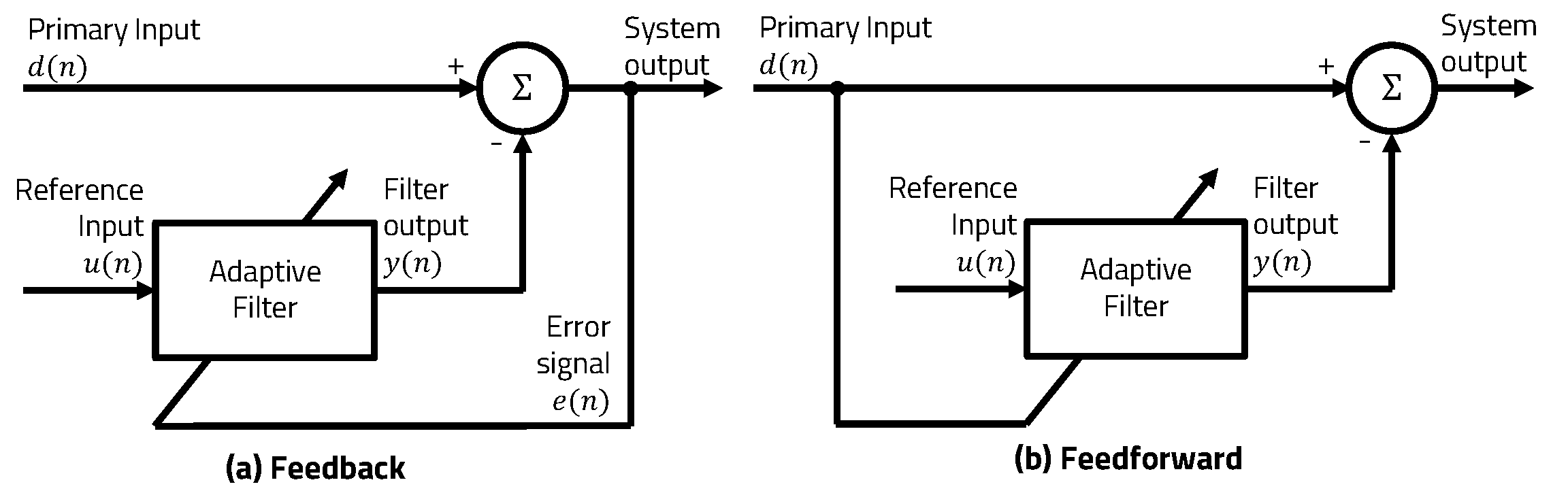
2. Related Work
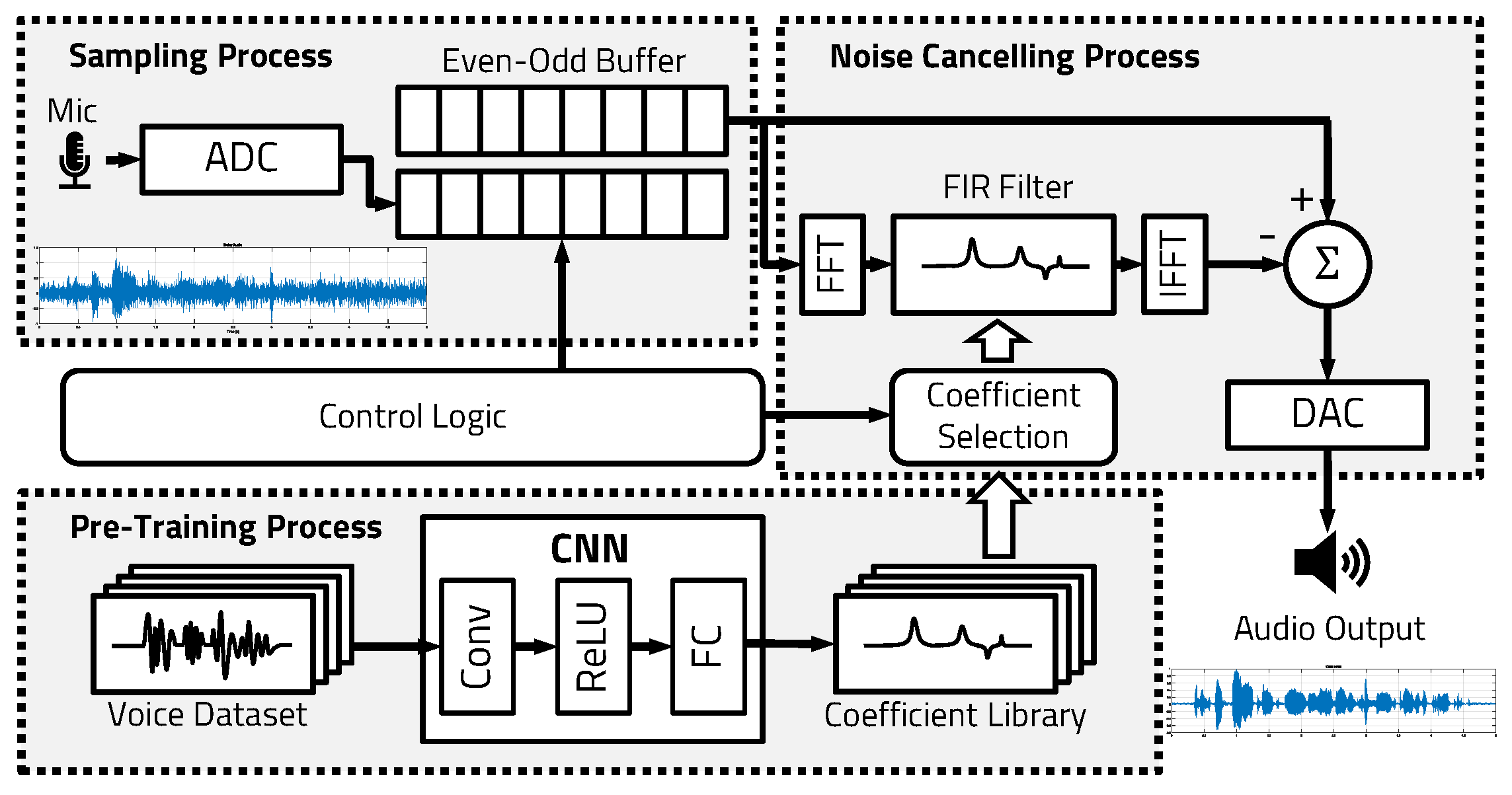
3. Proposed Method
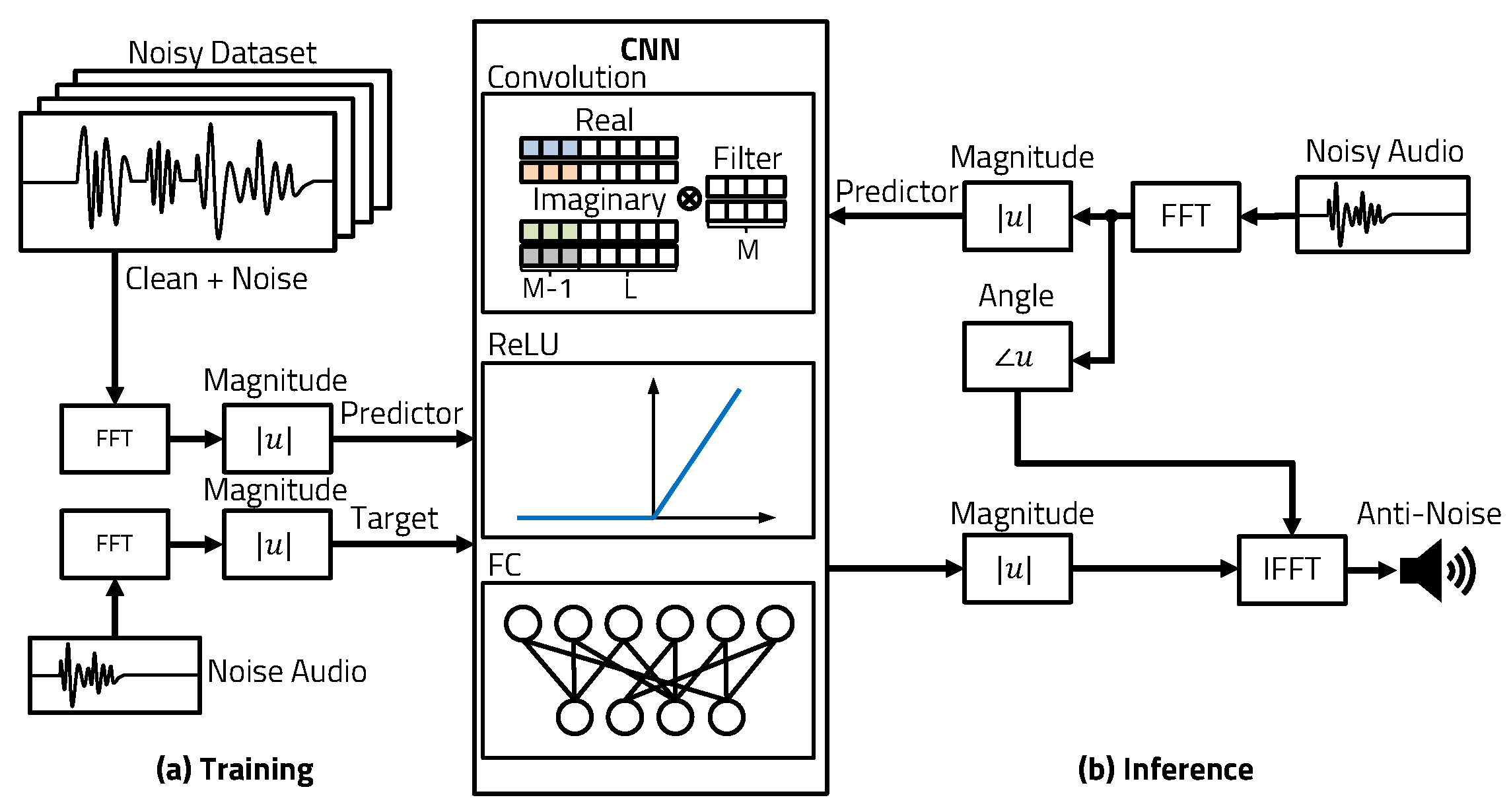
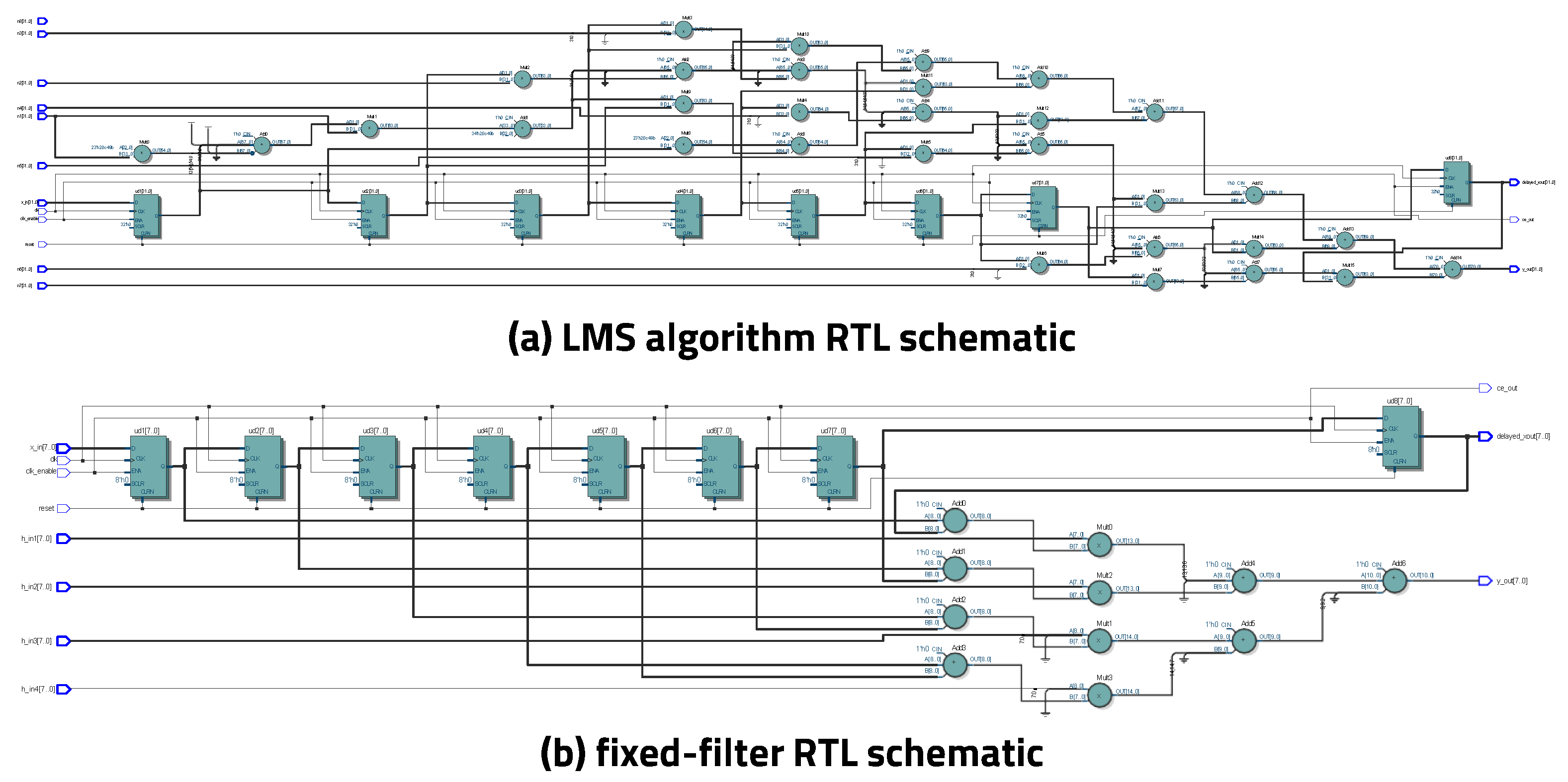
3.1. CNN Noise Cancellation
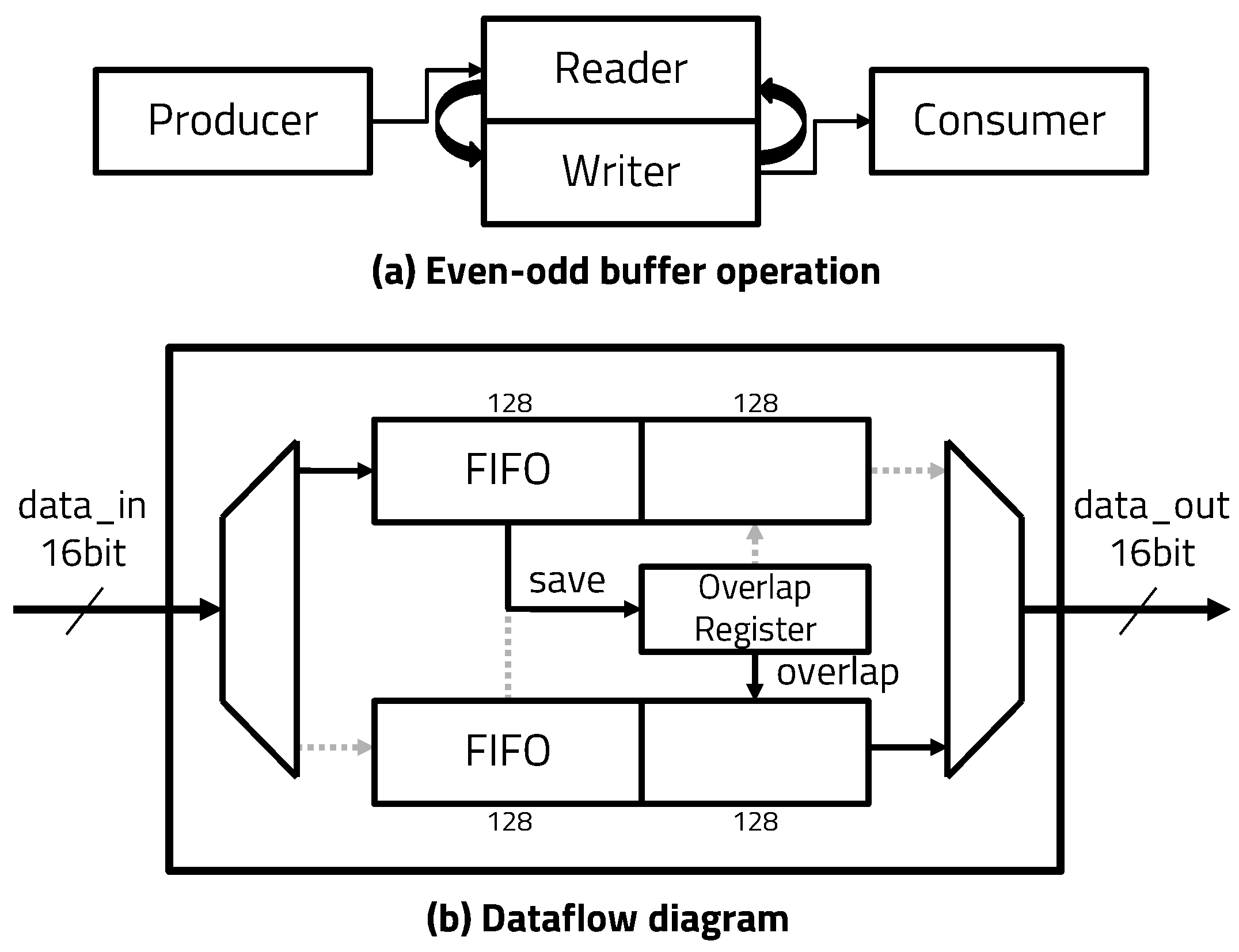
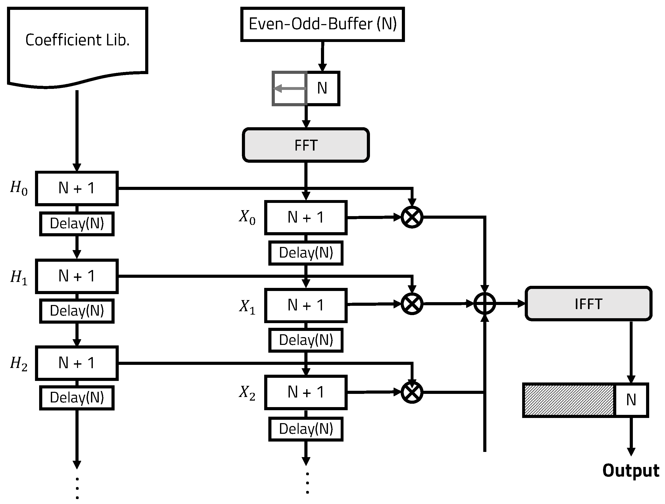
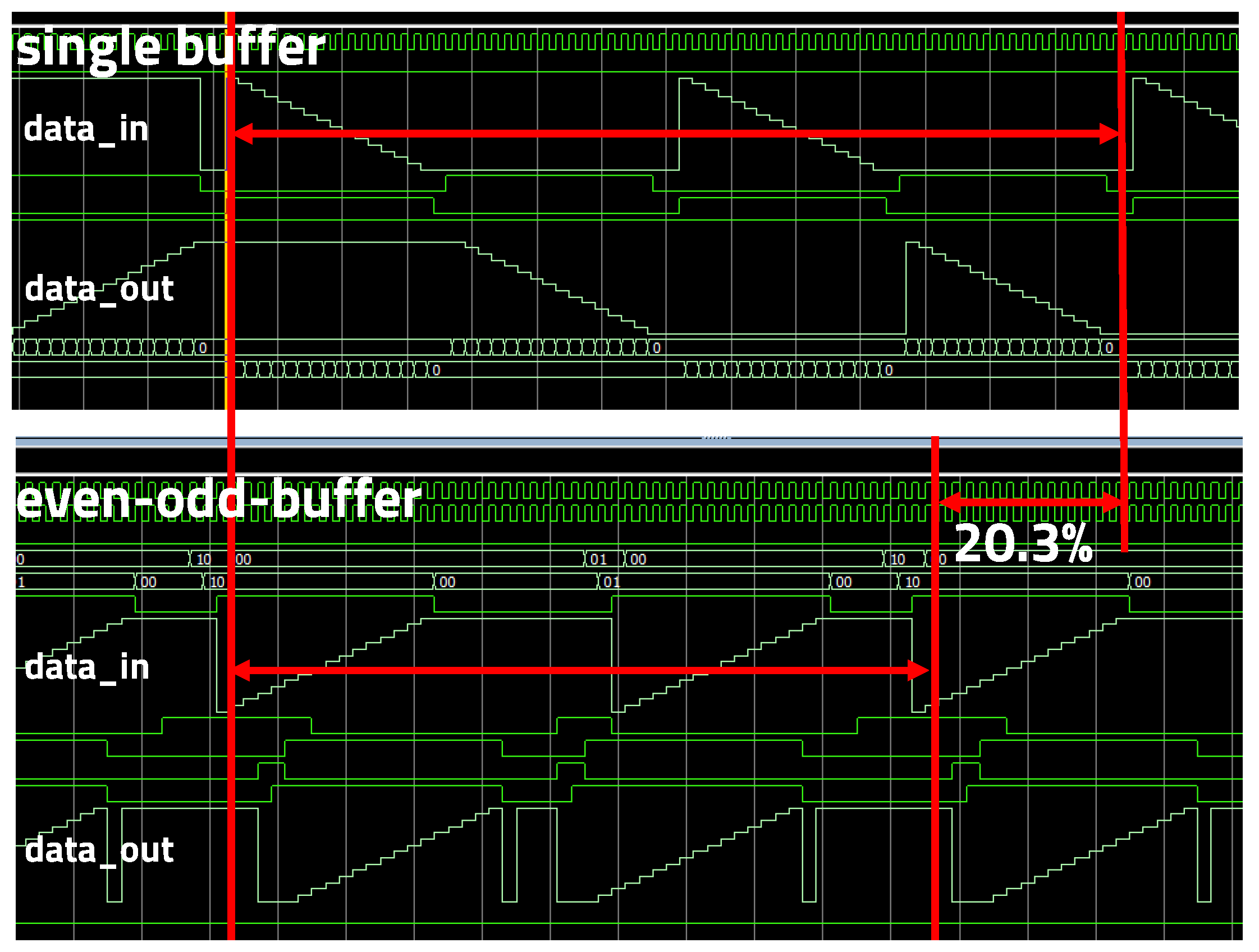
3.2. Even–Odd Buffer
| Algorithm 1 Even–odd buffering algorithm for the OLS convolution |
 |
3.3. Coefficient Selection Algorithm
| Algorithm 2 Coefficient selection algorithm for the noise classification |
 |
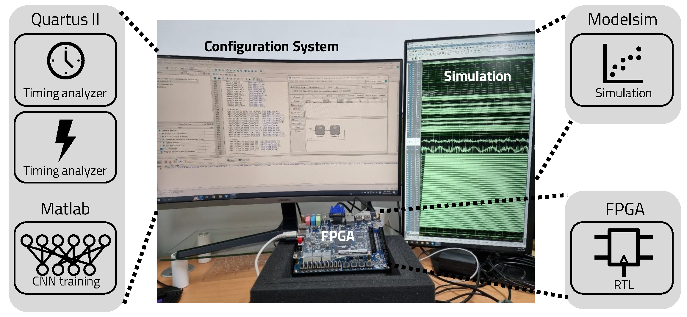
4. Experimental Setup
5. Evaluation
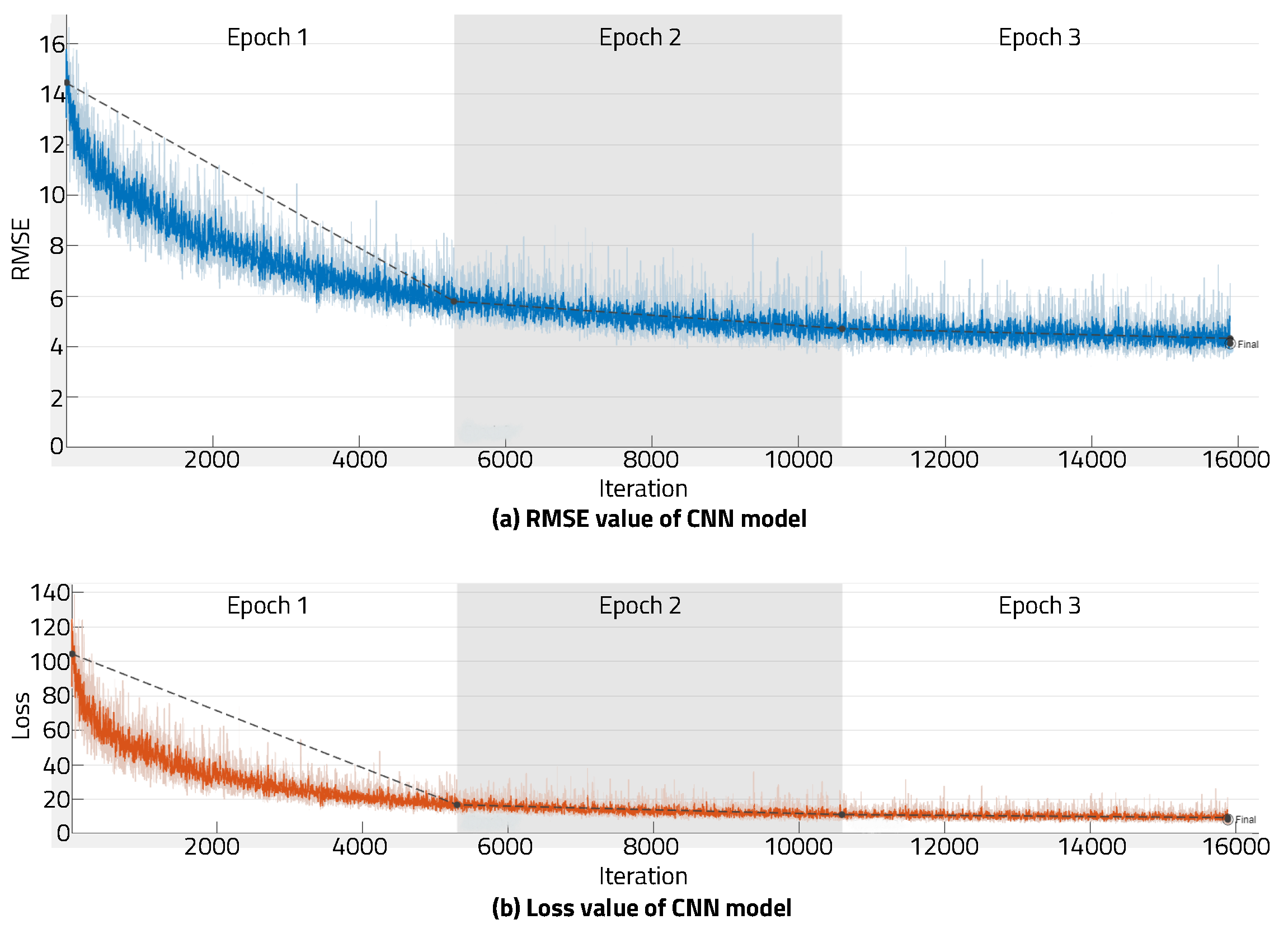
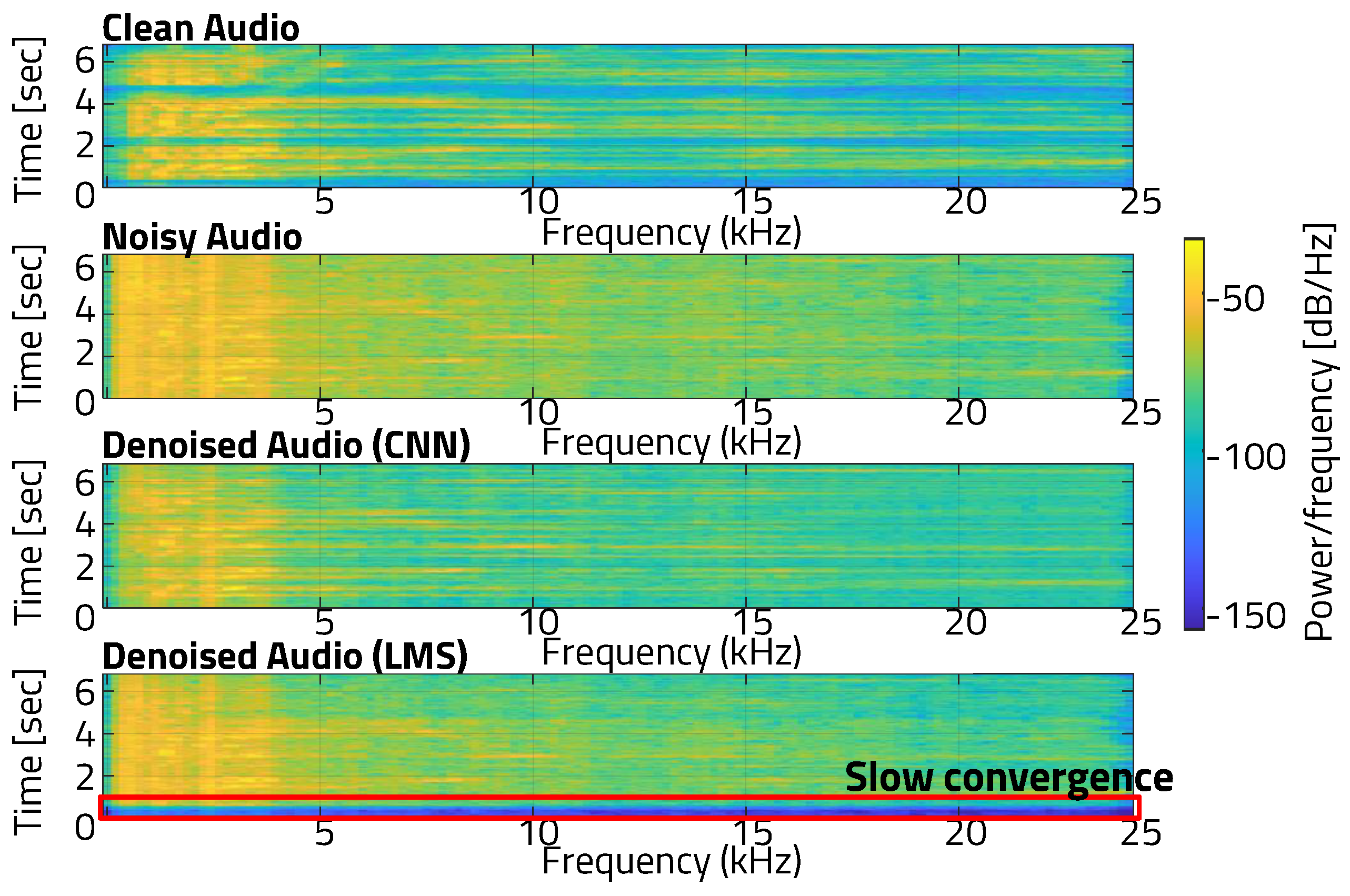
5.1. CNN Noise Cancellation
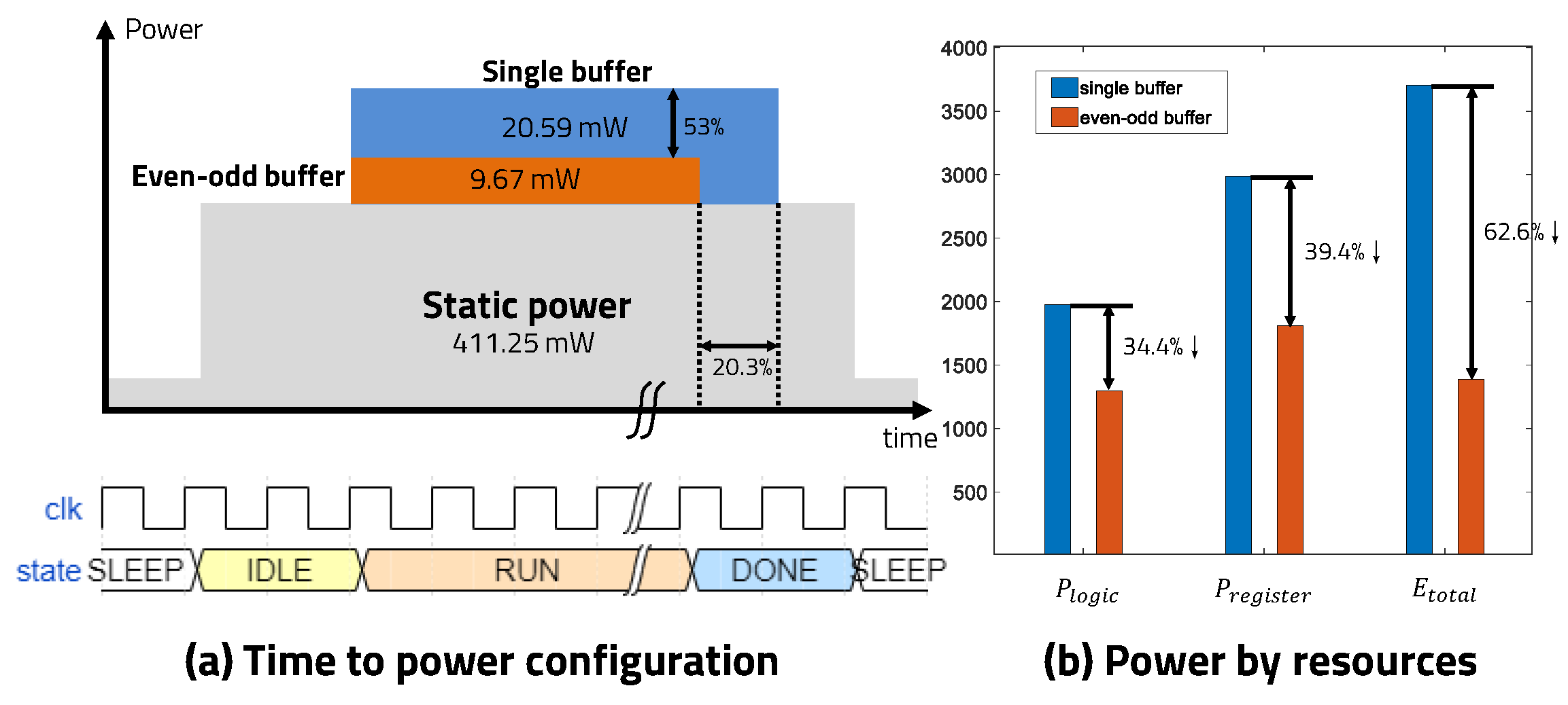
5.2. Even–Odd Buffer
6. Conclusions
Author Contributions
Funding
Conflicts of Interest
Abbreviations
| ANC | Active noise cancellation |
| DSP | Digital signal processing |
| LMS | Least mean square |
| CNN | Convolutional neural network |
| SNR | Signal-to-noise ratio |
| FFT | Fast Fourier transform |
| OLS | Overlap-save |
| FIR | Finite impulse response |
| HDL | Hardware description language |
| FPGA | Field-programmable gate array |
| RTL | Register transfer level |
| RMSE | Root mean square error |
References
- Elliott, S. Signal Processing for Active Control; Elsevier: Amsterdam, The Netherlands, 2000. [Google Scholar]
- Kuo, S.M.; Morgan, D.R. Active noise control: A tutorial review. Proc. IEEE 1999, 87, 943–973. [Google Scholar] [CrossRef]
- Bruschi, V.; Nobili, S.; Cecchi, S. A Real-Time Implementation of a 3D Binaural System based on HRIRs Interpolation. In Proceedings of the 2021 12th International Symposium on Image and Signal Processing and Analysis (ISPA), Zagreb, Croatia, 13–15 September 2021; pp. 103–108. [Google Scholar]
- Skarha, M. Performance Tradeoffs in HRTF Interpolation Algorithms for Object-Based Binaural Audio. Master’s Thesis, McGill University, Montreal, QC, Canada, 2022. [Google Scholar]
- Elliott, S.J.; Nelson, P.A. Active noise control. IEEE Signal Process. Mag. 1993, 10, 12–35. [Google Scholar] [CrossRef]
- Kajikawa, Y.; Gan, W.S.; Kuo, S.M. Recent advances on active noise control: Open issues and innovative applications. APSIPA Trans. Signal Inf. Process. 2012, 1, e3. [Google Scholar] [CrossRef]
- Haykin, S.S. Adaptive Filter Theory; Pearson Education: Noida, India, 2002. [Google Scholar]
- Jang, Y.J.; Park, J.; Lee, W.C.; Park, H.J. A Convolution-Neural-Network Feedforward Active-Noise-Cancellation System on FPGA for In-Ear Headphone. Appl. Sci. 2022, 12, 5300. [Google Scholar] [CrossRef]
- Perkell, J.S. Movement goals and feedback and feedforward control mechanisms in speech production. J. Neurolinguistics 2012, 25, 382–407. [Google Scholar] [CrossRef] [PubMed]
- Oosting, K.W. Simulation of Control Strategies for a Two Degree-of-Freedom Lightweight Flexible Robotic Arm. Ph.D. Thesis, Georgia Institute of Technology, Savannah, GA, USA, 1987. [Google Scholar]
- Shi, D.; Gan, W.S.; Lam, B.; Wen, S. Feedforward selective fixed-filter active noise control: Algorithm and implementation. IEEE/ACM Trans. Audio Speech Lang. Process. 2020, 28, 1479–1492. [Google Scholar] [CrossRef]
- Ma, Y.; Cao, Y.; Vrudhula, S.; Seo, J.s. Optimizing the convolution operation to accelerate deep neural networks on FPGA. IEEE Trans. Very Large Scale Integr. Syst. 2018, 26, 1354–1367. [Google Scholar] [CrossRef]
- Kapasi, U.J.; Mattson, P.; Dally, W.J.; Owens, J.D.; Towles, B. Stream Scheduling; Technical Report; Stanford Univeristy Computer Systems Lab.: Stanford, CA, USA, 2000. [Google Scholar]
- Shi, D.; Lam, B.; Ooi, K.; Shen, X.; Gan, W.S. Selective fixed-filter active noise control based on convolutional neural network. Signal Process. 2022, 190, 108317. [Google Scholar] [CrossRef]
- Park, S.; Park, D. Lightweighted FPGA Implementation of Even-Odd-Buffered Active Noise Canceller with On-Chip Convolution Acceleration Units. In Proceedings of the 2023 International Conference on Electronics, Information, and Communication (ICEIC), Singapore, 5–8 February 2023; pp. 1–4. [Google Scholar]
- Hershey, S.; Chaudhuri, S.; Ellis, D.P.; Gemmeke, J.F.; Jansen, A.; Moore, R.C.; Plakal, M.; Platt, D.; Saurous, R.A.; Seybold, B.; et al. CNN Architectures for Large-Scale Audio Classification. In Proceedings of the 2017 IEEE International Conference on Acoustics, Speech and Signal Processing (ICASSP), Chonburi, Thailand, 7–9 May 2017; pp. 131–135. [Google Scholar]
- Kwon, S. A CNN-assisted enhanced audio signal processing for speech emotion recognition. Sensors 2019, 20, 183. [Google Scholar]
- Sukhavasi, M.; Adapa, S. Music theme recognition using CNN and self-attention. arXiv 2019, arXiv:1911.0704. [Google Scholar]
- Caillon, A.; Esling, P. Streamable Neural Audio Synthesis With Non-Causal Convolutions. arXiv 2022, arXiv:2204.07064. [Google Scholar]
- Tsioutas, K.; Xylomenos, G.; Doumanis, I. Aretousa: A Competitive audio Streaming Software for Network Music Performance. In Proceedings of the 146th Audio Engineering Society Convention, Dublin, Ireland, 20–23 March 2019. [Google Scholar]
- Wright, W.E. Single versus double buffering in constrained merging. Comput. J. 1982, 25, 227–230. [Google Scholar] [CrossRef]
- Khan, S.; Bailey, D.; Gupta, G.S. Simulation of Triple Buffer Scheme (Comparison with Double Buffering Scheme). In Proceedings of the 2009 Second International Conference on Computer and Electrical Engineering, Dubai, United Arab Emirates, 28–30 December 2009; Volume 2, pp. 403–407. [Google Scholar]
- Daher, A.; Baghious, E.H.; Burel, G.; Radoi, E. Overlap-save and overlap-add filters: Optimal design and comparison. IEEE Trans. Signal Process. 2010, 58, 3066–3075. [Google Scholar] [CrossRef]
- Han, S.; Liu, X.; Mao, H.; Pu, J.; Pedram, A.; Horowitz, M.A.; Dally, W.J. EIE: Efficient inference engine on compressed deep neural network. ACM SIGARCH Comput. Archit. News 2016, 44, 243–254. [Google Scholar] [CrossRef]
- Capotondi, A.; Rusci, M.; Fariselli, M.; Benini, L. CMix-NN: Mixed low-precision CNN library for memory-constrained edge devices. IEEE Trans. Circuits Syst. II Express Briefs 2020, 67, 871–875. [Google Scholar] [CrossRef]
- Park, S. CNN ANC Data. Available online: https://github.com/SeunghyunPark0205/CNNANCDATA (accessed on 24 May 2023).
- Lee, S.; Lee, D.; Choi, P.; Park, D. Accuracy–power controllable lidar sensor system with 3D object recognition for autonomous vehicle. Sensors 2020, 20, 5706. [Google Scholar] [CrossRef] [PubMed]
- Park, S.; Park, D. Low-Power LiDAR Signal Processor with Point-of-Cloud Transformation Accelerator. In Proceedings of the 2022 IEEE International Conference on Consumer Electronics-Taiwan, Taipei, Taiwan, 6–8 July 2022; pp. 57–58. [Google Scholar]


| Processor | 12th-Gen Intel(R) Core(TM) i7-12700 KF, 3610 MHz, 12 Cores, 20 Logic Processors |
| Memory | 16 GB |
| Training Tool | MATLAB deep-learning toolbox |
| Epoch | 3 |
| Batch Size | 128 |
| Iteration | 15,888 |
| Learning Rate | 8 × |
| FFT Size | 256 |
| Window Length | 256 |
| LMS Algorithm | Fixed Filter | |
|---|---|---|
| Family | Cyclone V | Cyclone V |
| Device | 5CSEMA5F31C6N | 5CSEMA5F31C6N |
| Maximum clock frequency | 310.08 MHz | 717.36 MHz |
| Total pins | 71/457 | 60/457 |
| Logic utilization in ARM | 96/32,070 | 33/32,070 |
| Total registers | 145 | 64 |
| Dynamic power dissipation | 11.2 mW | 8.74 mW |
| Static power dissipation | 411.25 mW | 411.25 mW |
| Single Buffer | Even–Odd Buffer | |
|---|---|---|
| Family | Cyclone V | Cyclone V |
| Device | 5CSEMA5F31C6N | 5CSEMA5F31C6N |
| Total pins | 71/457 | 77/457 |
| Logic utilization in ARM | 96/32,070 | 134/32,070 |
| Total registers | 145 | 187 |
| Dynamic power dissipation | 20.59 mW | 9.67 mW |
| Static power dissipation | 411.25 mW | 411.25 mW |
Disclaimer/Publisher’s Note: The statements, opinions and data contained in all publications are solely those of the individual author(s) and contributor(s) and not of MDPI and/or the editor(s). MDPI and/or the editor(s) disclaim responsibility for any injury to people or property resulting from any ideas, methods, instructions or products referred to in the content. |
© 2023 by the authors. Licensee MDPI, Basel, Switzerland. This article is an open access article distributed under the terms and conditions of the Creative Commons Attribution (CC BY) license (https://creativecommons.org/licenses/by/4.0/).
Share and Cite
Park, S.; Park, D. Low-Power FPGA Realization of Lightweight Active Noise Cancellation with CNN Noise Classification. Electronics 2023, 12, 2511. https://doi.org/10.3390/electronics12112511
Park S, Park D. Low-Power FPGA Realization of Lightweight Active Noise Cancellation with CNN Noise Classification. Electronics. 2023; 12(11):2511. https://doi.org/10.3390/electronics12112511
Chicago/Turabian StylePark, Seunghyun, and Daejin Park. 2023. "Low-Power FPGA Realization of Lightweight Active Noise Cancellation with CNN Noise Classification" Electronics 12, no. 11: 2511. https://doi.org/10.3390/electronics12112511
APA StylePark, S., & Park, D. (2023). Low-Power FPGA Realization of Lightweight Active Noise Cancellation with CNN Noise Classification. Electronics, 12(11), 2511. https://doi.org/10.3390/electronics12112511