Improving the Accuracy of Lane Detection by Enhancing the Long-Range Dependence

Abstract

Lane detection is a common task in computer vision that involves identifying the boundaries of lanes on a road from an image or a video. Improving the accuracy of lane detection is of great help to advanced driver assistance systems and autonomous driving that help cars to identify and keep in the correct lane. Current high-accuracy models of lane detection are mainly based on artificial neural networks. Among them, CLRNet is the latest famous model, which attains high lane detection accuracy. However, in some scenarios, CLRNet attains lower lane detection accuracy, and we revealed that this is caused by insufficient global dependence information. In this study, we enhanced CLRNet and proposed a new model called NonLocal CLRNet (NLNet). NonLocal is an algorithmic mechanism that captures long-range dependence. NLNet employs NonLocal to acquire more long-range dependence information or global information and then applies the acquired information to a Feature Pyramid Network (FPN) in CLRNet for improving lane detection accuracy. Using the CULane dataset, we trained NLNet. The experimental results showed that NLNet outperformed state-of-the-art models in terms of accuracy in most scenarios, particularly in the no-line scenario and night scenario. This study is very helpful for developing more accurate lane detection models.

1. Introduction

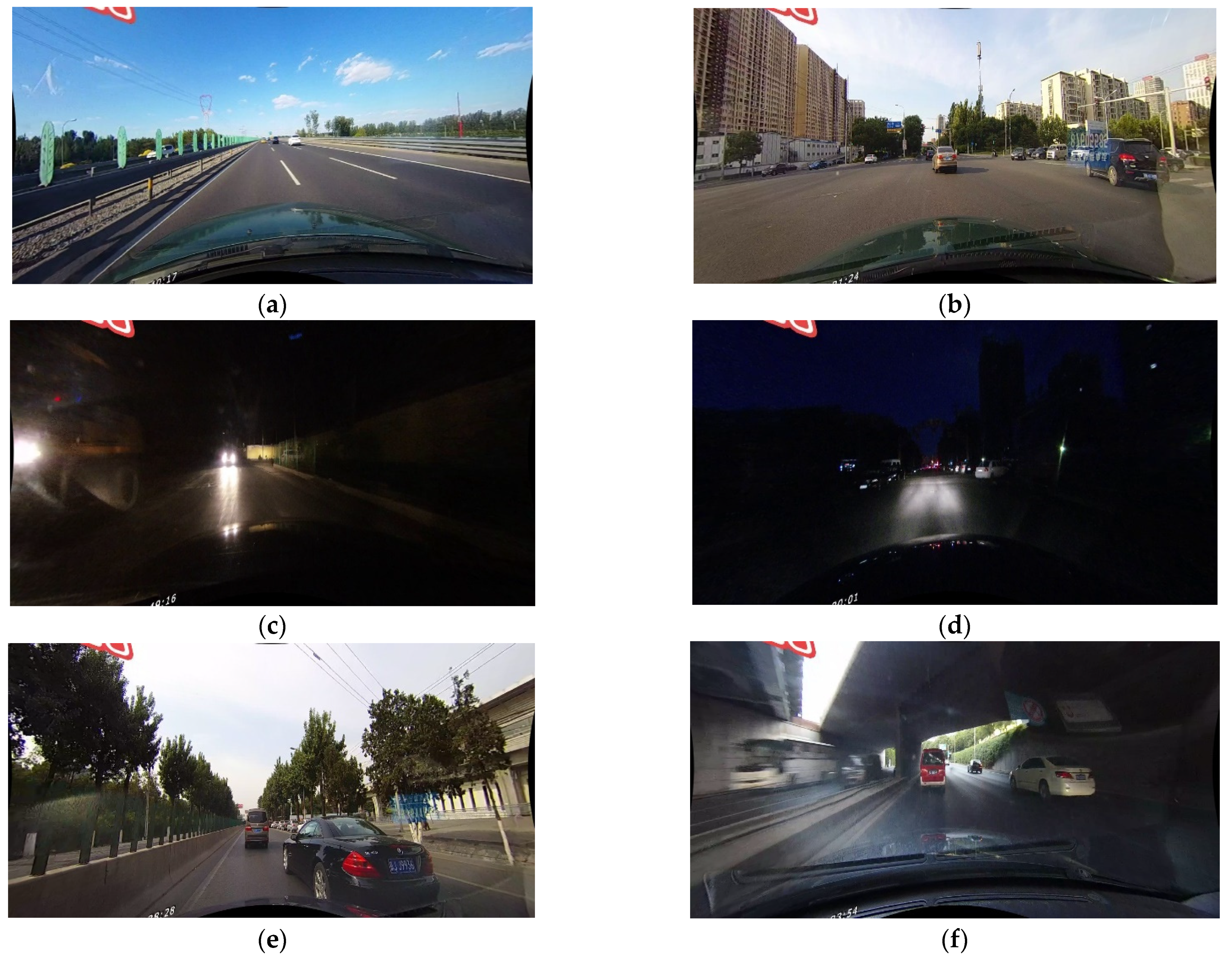
Lane detection aims to locate and identify the lane markings on a road surface from images or videos captured by cameras mounted on the vehicle. Lane detection can provide useful information for navigation, lane keeping, lane changing, collision avoidance, and traffic analysis [1]. However, due to the ever-changing road environment, the lane detection task is very complex [1,2]. For example, when lane lines are blocked by other vehicles on crowded roads, when night falls, or when the road does not mark the lane, it is very difficult to detect the lane. Sometimes the arrows on the road can also cause a decrease in detection accuracy because they will be incorrectly detected as lane lines. When there is glare and shadow [3] or when pedestrians cross a road at an intersection but there is no lane line on the ground, it will increase the difficulty of lane detection. In addition, there are even multiple conditions that affect the detection accuracy at the same time, such as dazzle on a road without lane lines at night. Figure 1 illustrates five of these practical scenarios that affect the accuracy of lane detection.

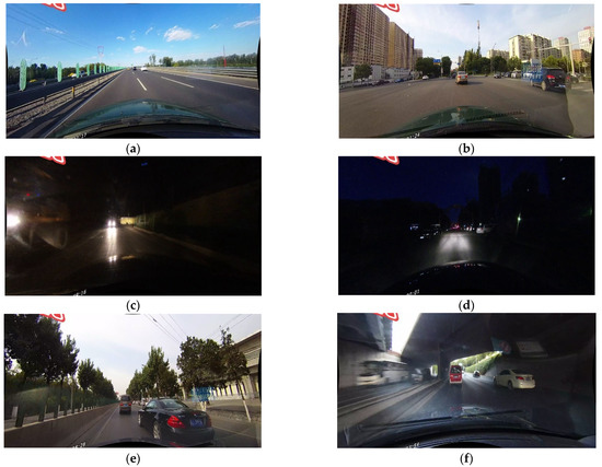
Figure 1. Illustrations of one ideal scenario and five difficult scenarios that affect the accuracy of lane detection. (a) The normal scenario that is easiest for lane detection. (b) The no-line scenario: when crossing the road at the intersection, there is no lane line on the ground, which affects the detection accuracy. (c) The dazzle scenario: the strong oncoming light causes the lane lines on the road to be blurred. (d) The night scenario. (e) The crowded scenario: lane lines are blocked by other vehicles on crowded roads, which will increase the difficulty of lane detection. (f) The shadow scenario.

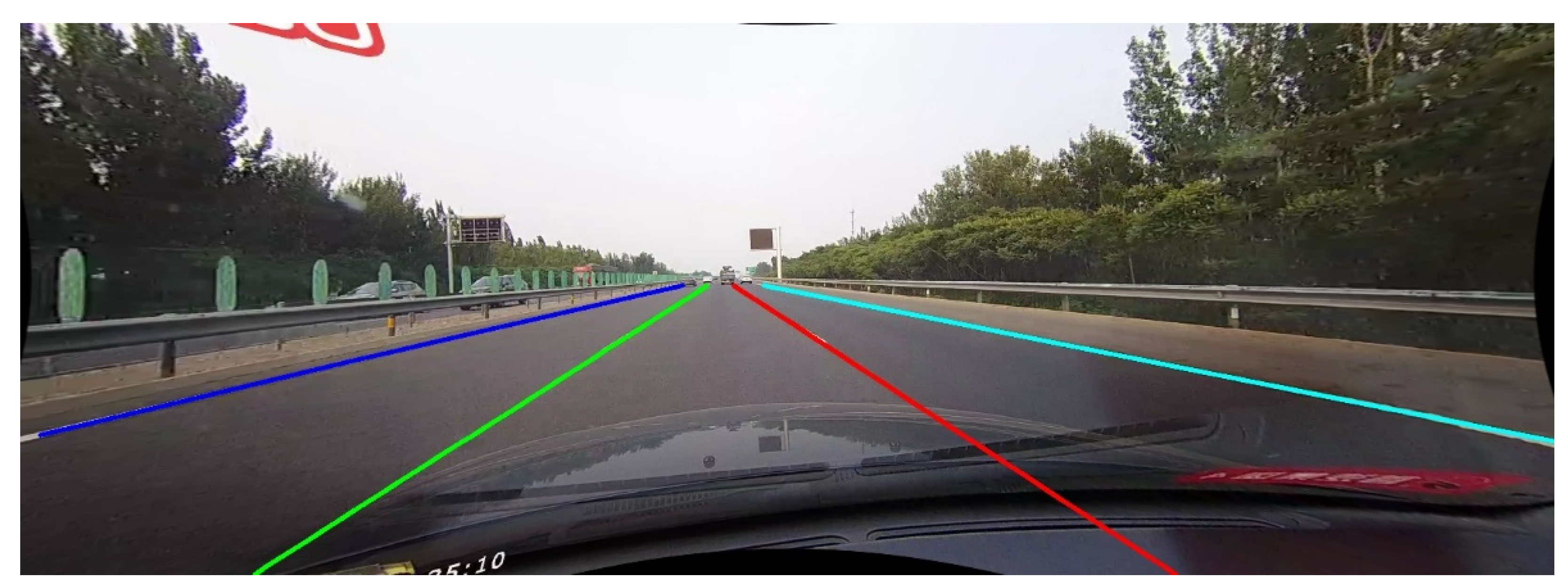
The core task of lane detection is to depict lane lines as accurately as possible in the image. Figure 2 shows the depiction of lane lines in the image: the blue, red, azure, and green lines in the figure are lane lines depicted with ground truth, and the lane lines depicted with the predicted results are similar to this.

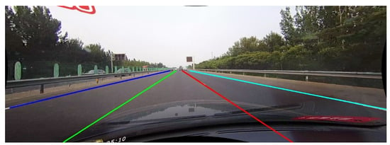
Figure 2. The depiction of lane lines in the image.

The methods of lane detection can be roughly divided into two categories: traditional methods and deep learning methods [4]. Traditional methods mainly use image processing techniques, such as edge detection, color threshold, perspective transformation, and Hough transformation, to extract and fit the features of lane lines. The advantage of this type of method is that it is fast, but the disadvantage is that it has poor robustness and is not suitable for complex scenes and lighting conditions [5]. Deep learning methods mainly use convolutional neural networks to learn semantic information about lane lines, such as segmentation, classification, and regression. In general, deep learning methods attain higher accuracy than traditional methods in various scenarios. Therefore, current research on lane detection mainly adopts artificial-neural-network-based models [6].

After carefully analyzing the abovementioned scenarios that affect the accuracy of lane detection, we found that the lane lines in these scenes are very context-dependent [6,7]. For example, when a car found that there were no lane lines on the ground in a short distance, but there were lane lines earlier, that is, the content of the context can be used to enhance the features of the lane lines, then the accuracy of lane detection will be improved. For example, in the dazzle scene, most of the time, the strong light from the oncoming car will pass by quickly and the lane lines before and after this are not disturbed by the strong light, and thus, they are relatively clear. Similarly, if the front and rear lane lines, that is, the context content, can be used to enhance the lane line features, the accuracy of lane detection in the shadow scenario will also be improved. Based on such observation and analysis, we proposed a nonlocal-based neural network model with the goal of achieving higher accuracy for lane detection. Specifically, we embedded the nonlocal [7] module into the FPN [8] (Feature Pyramid Network) of the CLRNet [6] model.

The FPN (Feature Pyramid Network) is a powerful deep learning architecture that can be used for various computer vision tasks, including object detection and semantic segmentation. It builds on the standard convolutional neural network (CNN) to generate multi-scale feature maps, which are then used for further analysis. The FPN module consists of several convolutional layers with different filter sizes and strides. Each layer produces a set of feature maps that correspond to a specific scale or level of the input image. By using the FPN architecture, developers can generate multi-scale feature maps that are useful for various computer vision tasks, leading to improved performance and accuracy in object detection and semantic segmentation, as well as other computer vision applications. In the CLRNet model, the FPN is used to enhance the effectiveness of image feature extraction. CLRNet (Cross-Layer Refinement Network for Lane Detection) is another deep learning architecture that can be used for lane detection in autonomous driving systems. It was introduced in 2022 by Tu Zheng et al. The CLRNet model is designed to perform lane detection in real time using a single camera sensor. The input image is processed by the model, which generates a set of feature maps that are useful for detecting lanes. The CLRNet model uses a cross-layer refinement mechanism to improve the accuracy and robustness of the lane detection algorithm. The model consists of several modules that work together to perform lane detection. The first module generates a feature vector from the input image using a CNN. The feature vector is then processed using a series of response functions that learn to adjust the intensity of each pixel in the feature vector based on its location in the image. The final module generates the lane boundaries by using the learned response functions. However, the output may contain false positives or false negatives due to the limitations of the current lane detection algorithms. To address this issue, the CLRNet model uses a cross-layer refinement mechanism that refines the output of the previous module based on feedback from other layers. This helps to improve the accuracy and robustness of the lane detection algorithm. By using the CLRNet model, developers can achieve high-quality lane detection in real time by using a single camera sensor. This can be useful for applications such as autonomous driving, where accurate lane detection is critical for safe navigation. Additionally, the CLRNet model can be used for research and development purposes, such as improving the performance of existing lane detection algorithms.

The main contributions of this research are threefold:

• We proposed a novel model, namely, NLNet, which aimed to further incorporate more long-range dependencies information. To the best of our knowledge, we are the first to apply a nonlocal module to the latest state-of-the-art model in the field of lane detection.
• Based on the analysis of the size of the feature map of each layer of the FPN of CLRNet, we creatively applied the nonlocal module directly to the L2 layer of the FPN to enhance the information about long-range dependence.
• Our proposed NLNet model achieved state-of-the-art performance on the CULane dataset in terms of accuracy.

2. Related Work

Traditional methods for lane detection usually rely on hand-crafted features and they often require the manual tuning of parameters and thresholds for different scenarios. Deep learning methods, on the other hand, can automatically learn high-level features from data without requiring much domain knowledge or human intervention.

Early methods that used deep learning for lane detection were convolutional neural network [9,10] (CNN)-based models, which are able to extract features from road images and then applied a sliding window approach to detect lane candidates. These methods achieved good results on simple scenarios but struggled with complex scenes and curved lanes.

To address the limitations of CNN-based methods, some researchers have adopted semantic segmentation techniques for lane detection. Semantic segmentation is a task that assigns a label to each pixel in an image, indicating the category of the object or region that the pixel belongs to. For lane detection, semantic segmentation can be used to classify each pixel as either lane or non-lane. For example, Pan et al. [9] proposed a spatial convolutional neural network (SCNN) that uses spatial-message-passing along horizontal and vertical directions to capture long-range dependencies and enhance feature representation. The SCNN was trained on two large-scale datasets: CULane and TuSimple [11], which contain diverse road scenes and challenging conditions. The SCNN outperformed previous methods on both datasets and achieved real-time performance. Compared with SCNN, the Recurrent Feature-Shift Aggregator [12] (RESA) uses another message-passing mechanism. The goal of RESA is that each pixel in the final output feature map can contain the information of other pixels. This is used to encode spatial context features. The specific approach is to slice the feature map in the two dimensions of H and W to obtain several slices. For slices along H, information can come from two directions, namely, slices above and below it, and different step sizes will be combined to aggregate information across slices. For slices along W, information can also come from two directions, namely, slices to the left and the right. The aggregation method involves simple addition, which first processes the source slice with a 1D convolution, then applies a nonlinear activation, and finally adds the result to the corresponding target slice. The number of convolution kernels and the number of channels are equal to the number of channels in the feature map. When slicing in the H direction, the one-dimensional convolution is sliding in the W direction, and when slicing in the W direction, the one-dimensional convolution is sliding in the H direction. The final results on CULane show that RESA achieves better detection accuracy than SCNN.

Instead of CNN, Jonah Philion et al. [13] introduced a novel fully convolutional model of lane detection that learns to decode lane structures instead of delegating structure inference to post-processing. A row-based lane detection task was adopted in the field of lane lines for the first time in End-to-End Lane Marker Detection [14] (E2E), where E2E aimed to distinguish the specific position of each lane in each line and achieved state-of-the-art results at that time (2020). Ultra-Fast Lane Detection [15] (UFLD) defines lane detection as finding a set of positions of lane lines in an image, that is, location selection and classification based on line directions. The detection speed of this model is fast. In addition, the model is not a fully convolutional form of segmentation, but a general classification based on fully connected layers, and the features it uses are global. In this way, the problem of the receptive field is directly solved, and for this method, the receptive field is the full image size when detecting the position of the lane line in a row. Therefore, there is no need for a complex information transmission mechanism to achieve good results. Experimental results on Tusimple and CULane show that the proposed method can achieve performance close to or better than the state-of-the-art method at ultra-fast speed.

The PINet [16] model combines key point detection and point cloud instance segmentation to successfully implement a new lane detection algorithm, which can be applied to any scene and detect any number of lane lines. Combined with the post-processing algorithm, the false detection rate is very low, and it has very strong robustness. Due to the keypoint detection method used, the model is smaller and has less computational overhead compared with the segmentation network.

An attention mechanism is also used in some models, such as the LaneATT [17] model, where it is able to use information from other lanes more easily by combining local and global features. The backbone of the model can be any generic CNN, such as Resnet, that takes the input image and generates feature maps. Subsequently, each anchor is projected onto the feature map. This projection is used to aggregate the features connected to another set of features created in the attention module. Finally, using the obtained feature set, two layers, namely, one for classification and the other for regression, are used to make the final prediction.

LaneAF [18] improves the pixel-by-pixel binary classification method for lane detection. Although there are some clustering or instance segmentation methods that can distinguish different lanes, they all have a limit to the maximum number of lanes that can be detected. Abualsaud Hala et al. proposed the LaneAF algorithm, which uses Affinity Field combined with a binary classification method for lane detection and instance segmentation. This method has good performance and can detect changes in the number of lane lines.

The SGNet [19] model introduces pixel-level perception, lane-level relation, and image-level attention constraints. Using these three parts of constraints on Anchor can obtain more accurate prediction results. Zhan Qu et al. [20] thought that the pixel-level output has information redundancy and at the same time will bring a lot of noise. Their proposed FOLOLane model uses two branches: one outputs a heatmap to determine whether the pixel is a key point and the other branch outputs offsets to accurately compensate for the position of the key point. The output network completes the local-to-global curve association through the association algorithm to form multiple complete curves.

The algorithm of the CondLaneNet [21] model is inspired by the instance segmentation algorithm CondInst. The core idea of the latter is to transform the instance segmentation problem from the previous scheme relying on boxes, ROI crops, and feature alignments to the learning scheme of the instance-sensitive convolution kernel parameters. CondLaneNet contains a proposal head and a conditional shape head. The proposal head is used to predict the lane line instance and the dynamic parameters of the convolution kernel at the instance level. The conditional shape head is used to predict the shape information of each lane line instance. CondLaneNet can solve the problem of lane line instance segmentation and crossing line detection and has good real-time performance.

In addition, transfer learning is a viable option for lane detection, and Ke Zhao et al. made significant contributions to this field through multiple papers. For instance, they proposed a federated multi-source domain adaptation method that combines transfer learning and federated learning for machinery fault diagnosis with data privacy [22]. Additionally, they developed a sophisticated transfer framework that employs an indirect latent alignment process to construct a common feature space using a Gaussian prior distribution instead of directly aligning the source and target distributions [23].

Moreover, some scholars have conducted in-depth research specifically for challenging scenarios. Xinxin Zhou et al. improved the performance of human detection in crowded scenarios by equipping FPN with multi-scale feature fusion technology and attention mechanisms. They designed a feature pyramid structure with a refined hierarchical split block, referred to as Scale-FPN, which can better handle the problem of scale variation across object instances. Furthermore, they proposed an attention-based lateral connection (ALC) module with spatial and channel attention mechanisms to replace the lateral connection in FPN, enhancing the representational ability of feature maps through rich spatial and semantic information. This enables detectors to focus on the important features of occlusion patterns [24].

Other scholars have also conducted research in related areas that have inspired the topic of lane detection. For example, driving fatigue seriously threatens traffic safety, and Fuwang Wang et al. proposed the multifractal detrended fluctuation analysis (MF-DFA) method to detect driver fatigue caused by driving for a long time [25]. Jiawei Xu et al. designed an architecture that analyzes the segmentation windows of three-second data to capture unique driving characteristics and then differentiate drivers based on that basis. The proposed model includes a fully convolutional network (FCN) and a squeeze-and-excitation (SE) block [26]. Lastly, Bo Jin et al. highlighted in reference [27] that the time–frequency information in the Hilbert spectrum can be utilized to extract the instantaneous characteristic frequency based on the marginal spectrum features to detect the objective [27].

3. The Proposed Model: NLNet

Considering the basic idea of improving the accuracy of lane detection by enhancing the context relationship and long-range dependence, the nonlocal module was considered to implement our idea in the existing excellent lane detection model. The nonlocal module has good performance and superior generalization of existing models by enhancing their ability to capture global context and long-range dependencies. This study applied this idea to the CLRNet model.

3.1. Motivation

In fact, in the CLRNet model, there are also ideas of global relations and long-range dependencies, such as the use of CNN and the proposal ROIgather, but we do not believe that CNN and ROIGather are sufficient for enhancing lane line features with global information and long-range dependencies [6]. CNNs struggle to capture global relationships and long-range dependencies for several reasons [7,8,22]. First, CNNs rely on local receptive fields, which means that each convolutional filter only operates on a small region of the input. This limits the ability of CNNs to aggregate information from distant regions and to model complex interactions between them. Second, CNNs use pooling operations to reduce the spatial resolution of the feature maps and to introduce some degree of translation invariance. However, pooling also discards some spatial information and may cause some loss of semantic information. Third, CNNs use a fixed number of convolutional layers with a fixed filter size and stride. This imposes a limit on the effective receptive field of each layer, which is the region of the input that influences the output of that layer. The effective receptive field grows linearly with the number of layers and quadratically with the filter size and stride. However, this growth may not be sufficient to cover the entire input or to capture long-range dependencies. Although the CLRNet model uses FPN to make up for the drawback that only local information can be obtained by using CNN alone, we do not believe that all the information about long-range dependence can be fully obtained in this way [28,29,30].

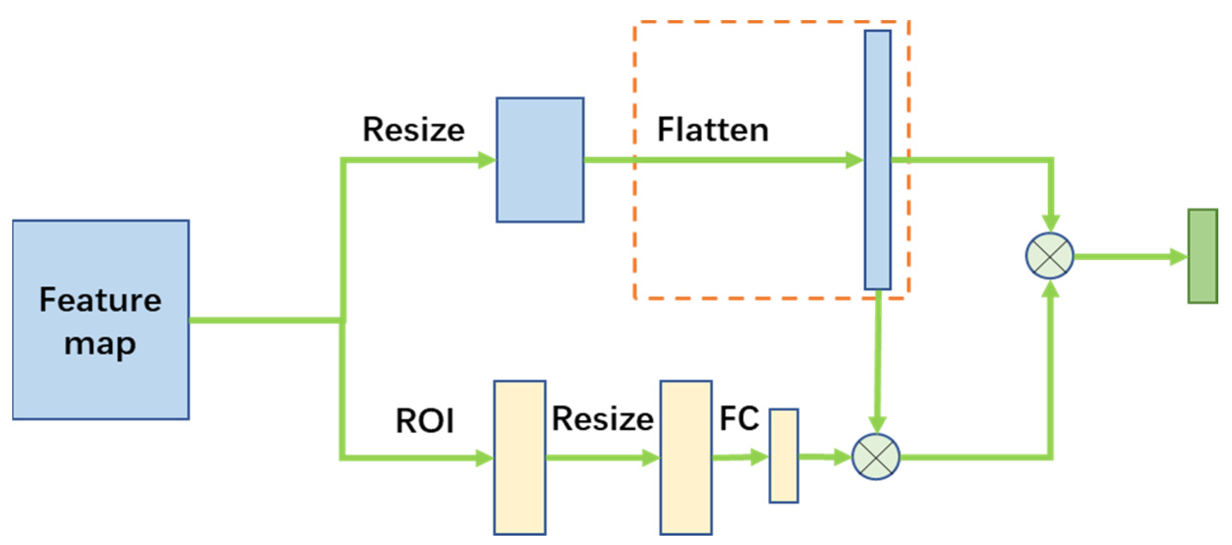
ROIGather is another technique used in the CLRNet model to extract long-range dependencies information. The architecture diagram of ROIGather is shown in Figure 3. Observing Figure 3, it can be found that CLRNet obtains the dependence between the lane line pixels and their surrounding pixels by continuing the convolution operation on the feature map of the ROI, and obtains the dependence between the lane line and the whole image by performing operations similar to the attention mechanism with the original feature map of the whole image. However, as shown in the red dashed box in Figure 3, the feature map is eventually flattened into a one-dimensional vector, thus losing the location information, which affects the final detection accuracy.

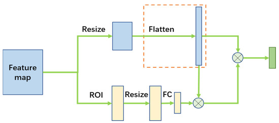
Figure 3. Architecture of ROIGather.

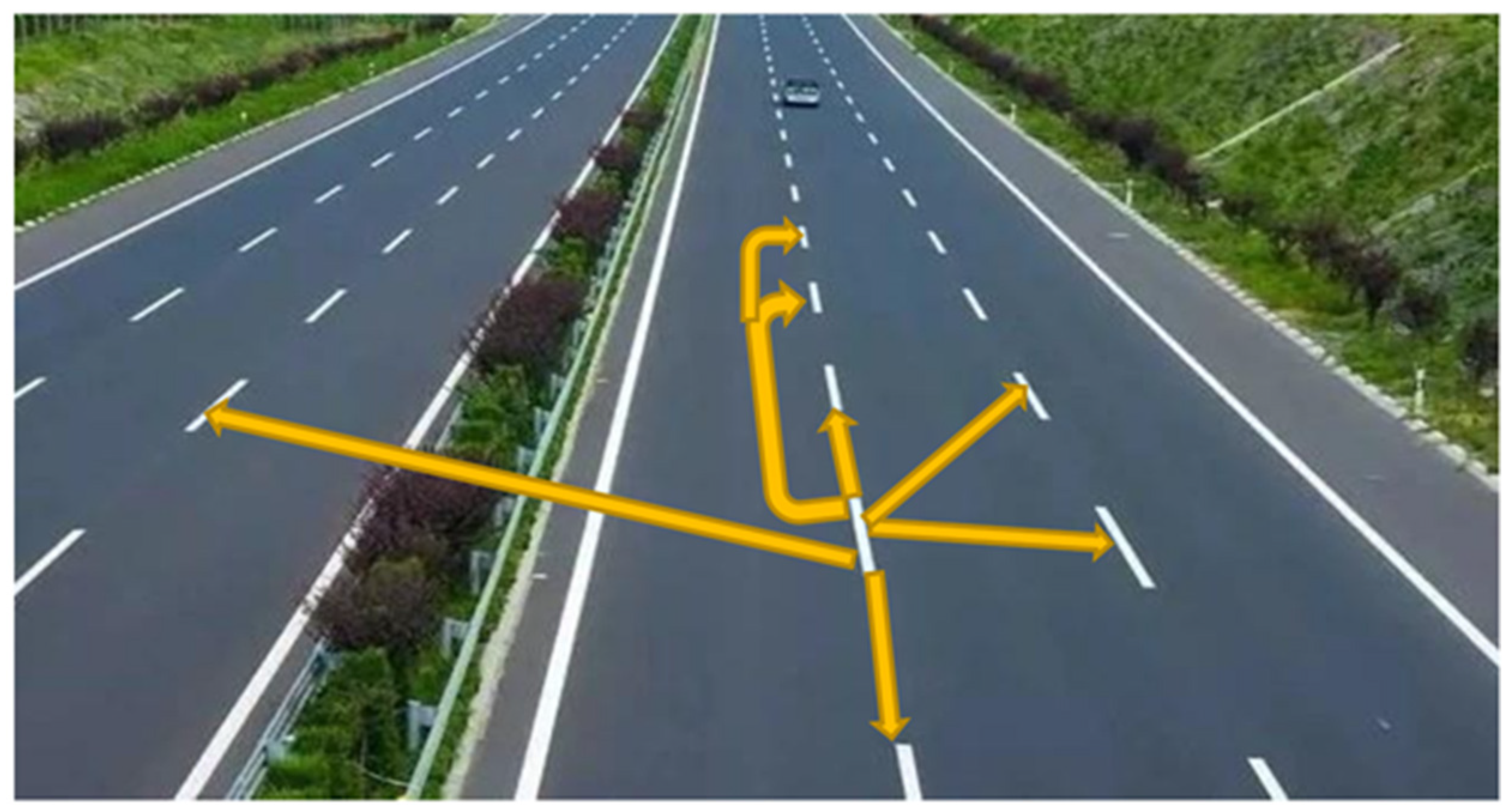
In summary, the CLRNet is not maximizing its use of the contribution of other global regions (e.g., pixels that are far away) to the current region. In fact, in a road image, the characteristics of each lane line can be enhanced through similarity. Specifically, pixels (no matter how far apart two pixels are) will enhance each other’s features due to their high similarity, and thus, the problem turns into obtaining the relationship weight of any pixel in the image to the current pixel, or in other words, capturing long-range dependencies. Figure 4 illustrates the similarity between a certain lane line and all other lane lines in the figure.

Figure 4. Illustration of the similarity between a certain lane line and all other lane lines (not all lane similarity arrows are drawn).

3.2. The Method for Obtaining Long-Range Dependencies

On the basis of CLRNet, it was the focus of our research to improve the detection accuracy by adding simple and effective long-range dependency modules. The nonlocal module is a neural network component that can capture long-range dependencies in data. It is inspired by the concept of nonlocal means, which is a denoising technique that uses the similarity of patches in an image to reduce noise. The nonlocal module has several advantages over conventional convolutional or recurrent layers. First, it can capture long-range dependencies without increasing the receptive field or the number of parameters. Second, it can adaptively adjust the weights based on the input data rather than using fixed kernels or weights. Third, it can handle variable-length inputs and outputs, such as sequences or graphs.

The basic idea of the nonlocal module is to compute a weighted sum of the features at all positions in the input, where the weights are determined by a pairwise function that measures the similarity or affinity between two positions. The output of the nonlocal module is then added to the original input as a residual connection, which helps to preserve the local information.

The nonlocal module can be formulated as follows:

$$y_i=\frac{{{\displaystyle \sum }}_{\forall j}f\left(x_i,x_j\right)g\left(x_j\right)}{c\left(x\right)}$$

where $y_i$ is the output feature at position $i$, $x_i$ is the input feature at position $i$, $f\left(x_i,x_j\right)$ is the pairwise function that computes the weight for position j given position $i$, and $g\left(x_j\right)$ is a function that transforms the input feature at position $j$. The summation is over all possible positions $j$ in the input.

The pairwise function $f$ can be implemented in different ways, such as using a dot product, Gaussian, embedded Gaussian, or concatenation. The $g$ function can be a linear projection or a more complex transformation. The nonlocal module can also be generalized to multi-head attention, where multiple output features are computed with different $g$ functions and then concatenated [7].

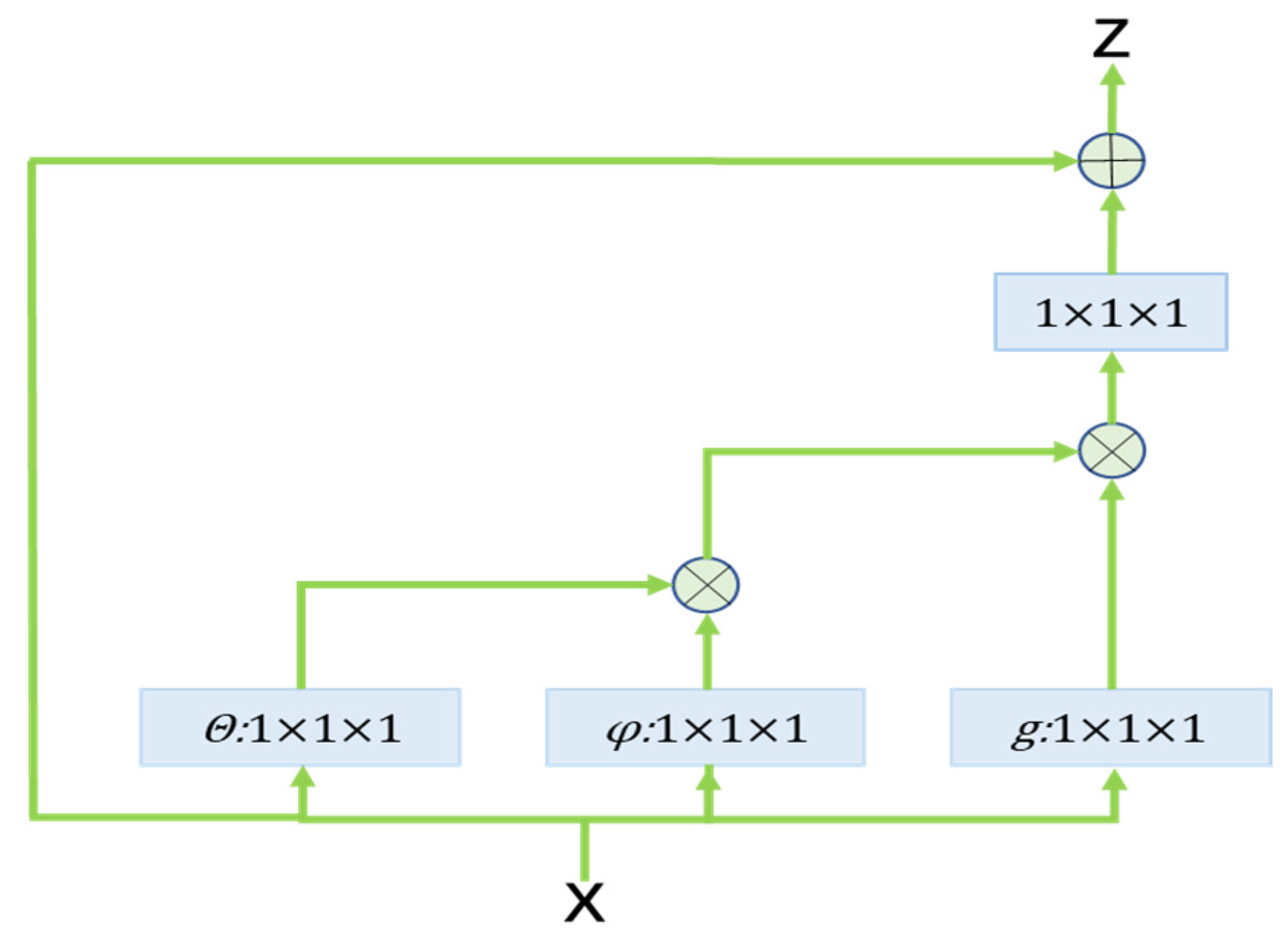
There are many ways to implement a nonlocal block, Figure 5 shows this concrete implementation of nonlocal. In this study, we did this through the following specific steps, as used in the original study.

Figure 5. Nonlocal implementation.

First, linear mapping is performed on the input feature map $X$ (essentially, 1 × 1 × 1 convolution is used to compress the number of channels), and then θ, φ, and g features are obtained.

Through the reshape operation, the dimensions of the above three features except the number of channels are forcibly merged, and then matrix dot multiplication of θ and φ is carried out to obtain something like a covariance matrix (this process is very important: the autocorrelation in the features are calculated, that is, the relationships between each pixel in each frame and all pixels in all other frames are obtained).

Then a softmax operation is performed on the autocorrelation features to obtain the weights from 0 to 1, which is the self-attention coefficient we need. Softmax is an activation function that normalizes a numeric vector to a probability distribution vector with probabilities adding up to 1. The formula for softmax is as follows, where $z$ is a vector and $z_i$ and $z_j$ are elements of it:

$$Softmax\left(z_i\right)=\frac{exp\left(z_i\right)}{{{\displaystyle \sum }}_{j}exp\left(z_j\right)}$$

Finally, the attention coefficient is multiplied back into the feature matrix g, and then the channel number is extended (1 × 1 × 1 convolution), and the residual operation is performed with the original input feature map X to obtain the output of the nonlocal block.

The steps above show that nonlocal directly integrates global information rather than simply obtaining a portion of global information by stacking multiple convolutional layers. This brings richer semantic information to the layers that follow.

3.3. NLNet

The network architecture of CLRNet is a cross-layer refinement network for lane detection that was proposed in a paper accepted by CVPR 2022. This network aims to fully utilize both high-level and low-level features in lane detection, and it is a state-of-the-art method that achieves impressive results on the CULane dataset. Therefore, we considered applying nonlocal ideas to CLRNet, and thus, a new model that we called NLNet was proposed.

Figure 6 shows the entire structure of the model. The road image in the lower-left corner of the figure is downsampled through P2, P3, and P4, and the CNN kernel window covers a larger observation area, thereby obtaining more high-level semantic information. From L0 to L2, upsampling is used, and we can see from Figure 2 that there are also horizontal connections between P2 and L2 and between P3 and L1. These horizontal connections will blend the high-level semantic information captured via downsampling with the low-level detail information captured by upsampling, ensuring that the model extracts more information. In addition, the head actually contains the ROIgather module, which uses a cross-layer refinement mechanism to refine the output of the previous module, ensuring that the model further extracts more information. Our contribution involved adding a nonlocal module (see the yellow dashed box in the figure), where the nonlocal module is a neural network component that can capture long-range dependencies in data. After all these feature extraction processes, the feature map is trained under the guidance of the loss function.

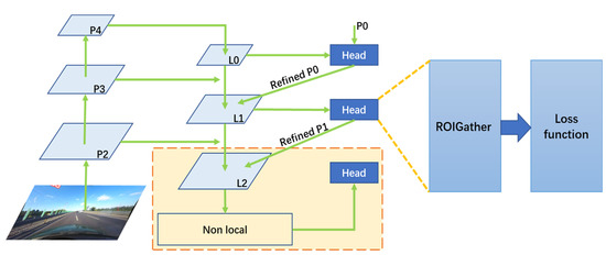
Figure 6. The entire structure diagram of the model.

The main idea of CLRNet is to first detect lanes with high-level semantic features, then perform refinement based on low-level features. In this way, it can exploit more contextual information to detect lanes while leveraging the local detailed lane features to improve localization accuracy.

Similar to CLRNet, the network architecture of NLNet consists of two main components: a feature pyramid network (FPN) and a cross-layer refinement module (CLRM). The FPN is used to extract multi-scale features from the input RGB image, and the CLRM is used to refine the lane detection results at each feature stage. The CLRM takes the current stage’s regression results as input and outputs refined regression results that are fed into the next stage. The CLRM also uses cross-layer connections to fuse features from different stages and enhance the feature representation. The FPN is composed of three stages: P2, P3, and P4. Each stage has a different spatial resolution and semantic level. The FPN adopts DLA34 as the backbone network and uses lateral connections to combine low-level and high-level features. The output of each stage is a feature map with 256 channels.

The overall workflow of NLNet is as follows: First, the input image is fed into the FPN to generate three feature maps: P2, P3, and P4. Then, each feature map is processed by the CLRM in a top-down manner, going from P4 to P2, which we named L0, L1, and L2. The CLRM is applied to each feature map separately and consists of two sub-modules: the cross-layer connection (CLC) and refinement head (RH). The CLC is a convolutional layer that takes the previous stage’s refined result as the input and outputs a feature map with the same resolution as the current stage. The RH is a convolutional layer that takes the current stage’s feature map and the CLC’s output as the input and outputs a refined result for the current stage. The fusion module is a convolutional layer that takes all the refined results as the input and outputs a fused result with the same resolution as P2. The output module is a convolutional layer that takes the fused result as the input and outputs a binary segmentation map for lane detection. The contribution of NCLNet is to enhance the long-range dependence of L2 with a nonlocal idea so that more global information can be obtained. The section in the red dotted box in Figure 6 shows the enhancement of the long-range dependencies on L2 using nonlocal.

Actually, the nonlocal model can be applied not only to L2 but also to L0 and L1; therefore, we can use nonlocal modules for L0, L1, and L2 at the same time, or only use nonlocal modules for one or two of L0, L1, and L2. Analyzing the workflow of NLNet, it is obvious that from L0 to L2, the size gradually increases. As the size of the feature map gradually decreases, the size of the lane line will also decrease at the same time, and too small of a lane line size will have a very poor effect on long-range dependence operations. Therefore, considering the tradeoff between the amount of calculation and the effect, nonlocal operation is only performed on L2.

We added a loss function in the CLRNet model, which means that the line $IOU$ loss is also used in our proposed model. The loss function designed in reference [6] was directly adopted, for each point in the predicted lane, we first extend it ($x_i^p$) with a radius $e$ into a line segment. Then $IOU$ can be calculated between the extended line segment and its ground truth, which is written as follows:

$$IOU=\frac{d_i^o}{d_i^u}=\frac{min\left(x_i^p+e, x_i^g+e\right)-max\left(x_i^p-e, x_i^g-e\right)}{max\left(x_i^p+e, x_i^g+e\right)-min\left(x_i^p-e, x_i^g-e\right)}$$

where $x_i^p-e$ and $x_i^p+e$ are the extended points of $x_i^p$, while $x_i^g-e$ and $x_i^g+e$ are the corresponding ground truth points. Note that $d_i^o$ can be negative, which can make it feasible to optimize in the case of non-overlapping line segments. Then $LIOU$ can be considered as the combination of infinite line points. The discrete form can be written as follows:

$$LIOU=\frac{{{\displaystyle \sum }}_{i=1}^N{d}_i^o}{{{\displaystyle \sum }}_{i=1}^N{d}_i^u}$$

Then, the $LIOU$ loss is defined as

$$L_{LIOU}=1-LIOU$$

where $-1\le LIOU\le 1$; when two lines overlay perfectly, then $LIOU=$ 1, and $LIOU$ converges to −1 when two lines are far away.

4. Training and Testing

4.1. Dataset

Considering the fairness of the comparison and the popularity of the dataset, the CULane dataset was chosen for the training and testing.

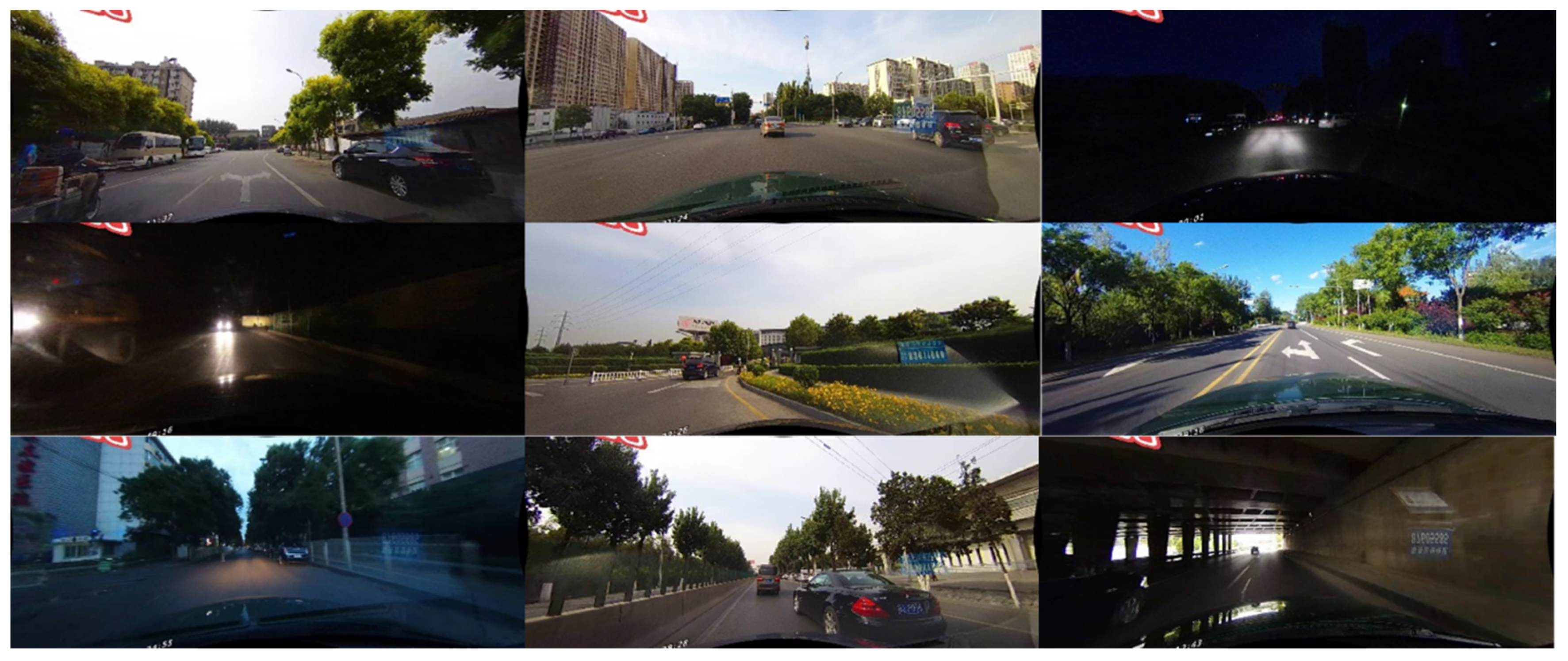
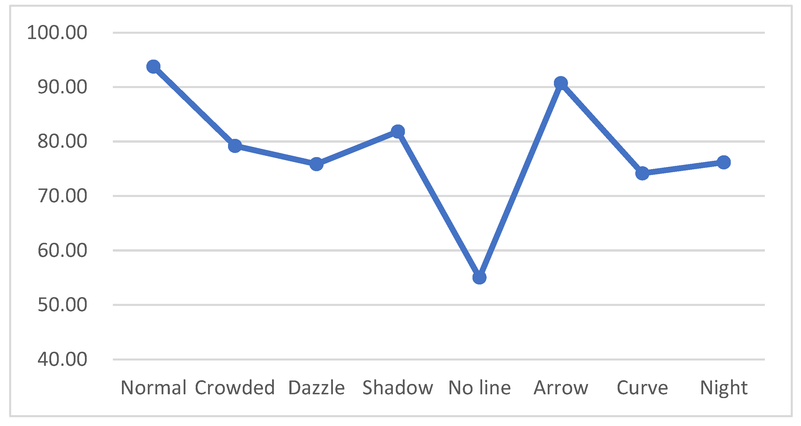
The CULane dataset is a large-scale challenging dataset for academic research on traffic lane detection. It was collected by cameras mounted on six different vehicles driven by different drivers in Beijing. More than 55 h of videos were collected and 133,235 frames were extracted. The dataset aims to provide a realistic and diverse benchmark for evaluating lane detection algorithms. It was divided into 88,880 images for the training set, 9675 for the validation set, and 34,680 for the test set; Figure 7 visually shows the ratios of the three sets. The test set was further divided into normal and eight challenging categories; Table 1 illustrates the categories and Figure 8 shows these scenarios.

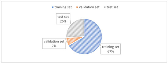
Figure 7. The ratios of the training set, validation set, and test set in the CULane dataset.

Table 1. Information about the CULane dataset.

Set	Quantity	Normal and Eight Challenging Categories
Training set	88,880	Normal: normal driving conditions with clear lane markings.
		Crowded: crowded traffic scenes with many vehicles.
		Night: night scenes with low illumination.
		No line: scenes where lane markings are missing or very faint.
		Shadow: scenes where shadows cast by vehicles or buildings obscure lane markings.
		Arrow: scenes where arrow markings indicate lane changing or turning.
		Curve: scenes where lanes are curved or bendy.
		Crossroad: scenes where multiple roads intersect or merge.
		Dazzle light: There are strong light sources on the road, such as headlights or sunlight, which may cause glare or reflection.
Validation set	9675
Test set	34,680

Figure 8. Normal and eight challenging scenarios.

For each image, the dataset provides a corresponding annotation file in the .txt format. Each line in the annotation file gives the x- and y-coordinates for key points of a lane marking. For cases where lane markings are occluded by vehicles or are unseen, the annotations still follow the lanes according to the context.

The dataset focuses on the detection of four lane markings that are most relevant for driving applications. Other lane markings are not annotated. The four lane markings are ordered from left to right as follows:

• Left-most lane marking: the left boundary of the left-most drivable lane.
• Left lane marking: the right boundary of the left-most drivable lane.
• Right lane marking: the left boundary of the right-most drivable lane.
• Right-most lane marking: the right boundary of the right-most drivable lane.

For each image, the dataset also provides a per-pixel label file in the .png format, which is generated from the original annotation files. The label file assigns a different color to each of the four lane markings and a black background to other regions. The label file can be used for training or evaluating semantic segmentation models for lane detection.

4.2. Hyperparameter Setting and Training

The environmental parameters of the training model are shown in Table 2. We employed the PyTorch 1.8 framework and Ubuntu 18 operating system to train our model. We utilized CUDA Version 10.2, CUDNN version 8.0, and Python version 3.8, and selected AdamW as the optimizer. To be precise, we conducted extensive experimentation and training for the hyperparameter tuning, with empirical observation being the fundamental approach. The model was trained for 25 epochs using a cosine decay learning rate strategy, where the power was set to 0.9. During the first 18 epochs, the learning rate was 0.6 × 10⁻³, while the remaining epochs used a learning rate of 0.2×10⁻³. In addition, we observed overfitting after the trained epochs exceeded 25.

Table 2. Training environment.

Tools or Libraries	Version
PyTorch	1.8
Ubuntu	18.04.1
CUDA	10.2
CUDNN	8
Python	3.8

5. Experiment Results and Discussion

5.1. Evaluation Indicators

The F1 score is a harmonic mean of precision and recall, which are two metrics that are commonly used to evaluate binary classification problems [23]. Precision measures how many of the positive predictions made by a model are correct, while recall measures how many of the positive examples in the data are correctly identified by the model. The F1 score combines these two metrics into a single number that ranges from 0 to 1, where 1 means perfect precision and recall, and 0 means no positive predictions or detections. The F1 score can be calculated as follows:

$$F1=2\times \left(precision\times recall\right) / \left(precision+recall\right)$$

To apply the F1 score to image detection models, we needed to define what constitutes a positive prediction and a positive example. In image detection, a model outputs a set of bounding boxes with class labels and confidence scores for each image. A positive prediction is a bounding box that matches a ground truth bounding box of the same class with a certain degree of overlap, usually measured by the intersection over union (IoU) metric. A positive example is a ground truth bounding box that is matched by a prediction of the same class with a certain IoU threshold.

Since the CULane dataset has nine road scenarios, the final test results were compared under these nine scenarios, and the overall indicators were mF1, $F1@50$, and $F1@50$.

To calculate precision and recall for image detection models, we needed to sort the predictions by their confidence scores in descending order and compare them with the ground truth bounding boxes using the IoU metric. For each prediction, we could assign it as a true positive ($TP$), false positive (FP), or false negative (FN) based on whether it matched a ground truth bounding box or not. Then, we could compute the cumulative precision and recall values for each prediction as follows:

$$Precision=TP/\left(TP+FP\right)$$

$$Recall=TP/\left(TP+FN\right)$$

Finally, we could plott the precision–recall ($PR$) curve by plotting the precision values against the recall values for each prediction. The $F1$ score could be obtained by finding the maximum value of the harmonic mean of precision and recall along the $PR$ curve.

The $F1$ score is useful for evaluating image detection models because it balances the trade-off between precision and recall. A high $F1$ score indicates that the model can detect most of the objects in the images with high accuracy and low false positives. In conclusion, the $F1$ score is a simple and intuitive metric that can be used to evaluate image detection models by combining precision and recall into a single number.

Following the CLRNet detection metric, the metric mF1 was also adopted in this study, where it is defined as

$$mF1=\left(F1@50+F1@55+···+F1@95\right)/10$$

where $F1@50,F1@55,···,F1@95$ are the $F1$ metrics when the IoU thresholds are 0.5, 0.55, · · ·, 0.95, respectively.

5.2. Test Results

CLRNet is a family of models that is composed of four models. The main difference between the four models is that they use different backbones, which are Resnet18, Resnet34, Resnet101, and DLA34. Among them, the model with the best detection accuracy is DLA34 as the backbone model. For the sake of comparison fairness, we chose CLRNet with DLA34 as the backbone to compare with NCLNet. The test results of our proposed model on CULane were compared with other benchmarks. Compared with the current best benchmark (CLRNet with DLA34 as backbone), we found that NLNet improved mF1 from 55.64 to 55.75, and improved F1@75 from 62.78 to 63.16. The precision of the dazzle condition was increased from 75.30 to 75.85, the precision of the no-line condition was increased from 54.58 to 55.03, and the precision of the night condition was increased from 75.37 to 76.17. Table 3 shows the test results of the NLNet model and the detailed data compared with other mainstream benchmarks; for the cross-scenario, only FP values are shown. The experiment results demonstrate that the NCLNet model greatly outperformed the state-of-the-art lane detection approaches. Figure 9 shows the comparison of the visualization results under different conditions of our proposed model.

Table 3. Comparison of the experimental results.(the bold is to highlight the best experimental results).

Method	Backbone	mF1	F1@50	F1@75	FPS	Normal	Crowded	Dazzle	Shadow	No Line	Arrow	Curve	Cross	Night
SCNN	VGG16	38.84	71.60	39.84	7.5	90.60	69.70	58.50	66.90	43.40	84.10	64.40	1990	66.10
RESA	ResNet34	-	74.50	-	45.5	91.90	72.40	66.50	72.00	46.30	88.10	68.60	1896	69.80
RESA	ResNet50	47.86	75.30	53.39	35.7	92.10	73.10	69.20	72.80	47.70	88.30	70.30	1503	69.90
FastDraw	ResNet50	-	-	-	90.3	85.90	63.60	57.00	69.90	40.60	79.40	65.20	7013	57.80
E2E	ERFNet	-	74.00		-	91.00	73.10	64.50	74.10	46.60	85.80	71.90	2022	67.90
UFLD	ResNet18	38.94	68.40	40.01	282	87.70	66.00	58.40	62.80	40.20	81.00	57.90	1743	62.10
UFLD	ResNet34		72.30	-	170	90.70	70.20	59.50	69.30	44.40	85.70	69.50	2037	66.70
PINet	Hourglass	46.81	74.40	51.33	25	90.30	72.30	66.30	68.40	49.80	83.70	65.20	1427	67.70
LaneATT	ResNet18	47.35	75.13	51.29	153	91.17	72.71	65.82	68.03	49.13	87.82	63.75	1020	68.58
LaneATT	ResNet34	49.57	76.68	54.34	129	92.14	75.03	66.47	78.15	49.39	88.38	67.72	1330	70.72
LaneATT	ResNet122	51.48	77.02	57.5	20	91.74	76.16	69.47	76.31	50.46	86.29	64.05	1264	70.81
LaneAF	ERFNet	48.6	75.63	54.53	24	91.10	73.32	69.71	75.81	50.62	86.86	65.02	1844	70.90
LaneAF	DLA34	50.42	77.41	56.79	20	91.80	75.61	71.78	79.12	51.38	86.88	72.70	1360	73.03
SGNet	ResNet18	-	76.12	-	117	91.42	74.05	66.89	72.17	50.16	87.13	67.02	1164	70.67
SGNet	ResNet34	-	77.27	-	92	92.07	75.41	67.75	74.31	50.90	87.97	69.65	1373	72.69
FOLOLane	ERFNet	-	78.80	-	40	92.70	77.80	75.20	79.30	52.10	89.00	69.40	1569	74.50
CondLane	ResNet18	51.84	78.14	57.42	173	92.87	75.79	70.72	80.01	52.39	89.37	72.40	1364	73.23
CondLane	ResNet34	53.11	78.74	59.39	128	93.38	77.14	71.17	79.93	51.85	89.89	73.88	1387	73.92
CondLane	ResNet101	54.83	79.48	61.23	47	93.47	77.44	70.93	80.91	54.13	90.16	75.21	1201	74.80
CLRNet	DLA34	55.64	80.47	62.78	94	93.73	79.59	75.30	82.51	54.58	90.62	74.13	1155	75.37
NLNet(ours)	DLA34	55.75	80.49	63.16	83	93.74	79.19	75.85	81.83	55.03	90.69	74.14	1291	76.17

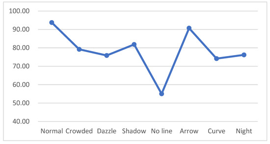
Figure 9. The comparison of the visualization results from the NLNet model under different conditions.

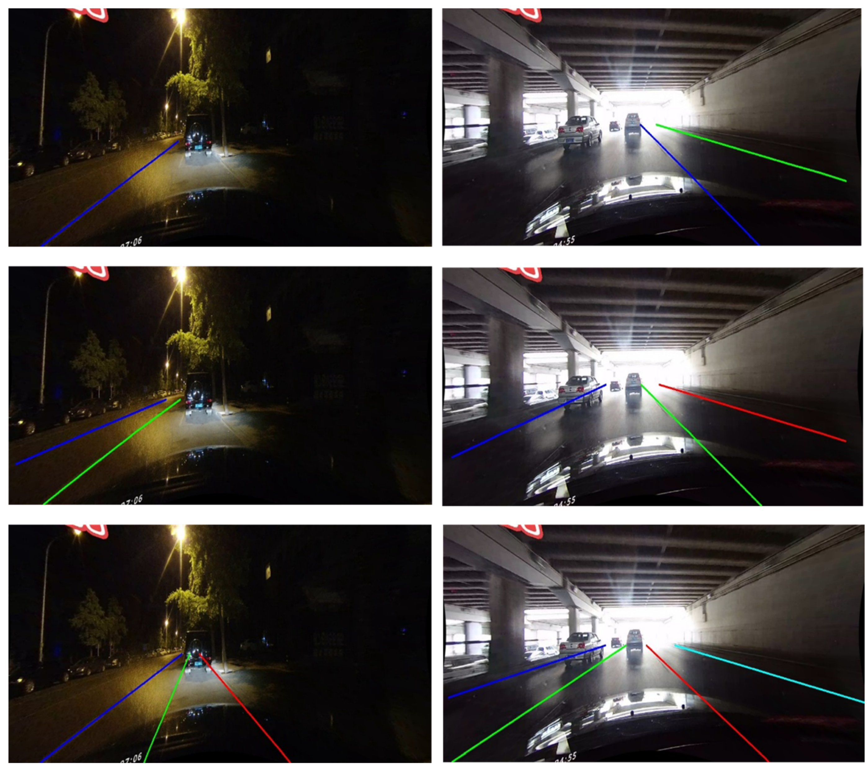
In order to see the effect of model detection more intuitively, we visualized the detection results of CLRNet on the test set of CULane. Figure 10 shows the comparison between the image with ground truth, the image with the lane line detected using CLRNet, and the image with the lane line detected using NLNet. Figure 10 has a total of six images, which are divided into two columns, where each column is a group of comparison objects; from top to bottom, the detection results of CLRNet, the detection results of NLNet, and the ground truth are shown. It can be found that the results of NLNet were consistent with the ground truth, while CLRNet did not detect all lane lines in the image.

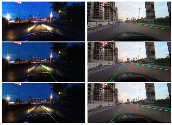
Figure 10. Comparison between the image with the lane line detected using CLRNet, the image with the lane line detected using NLNet, and the image with the ground truth.

Although our proposed model achieved the state-of-the-art effect, by observing Figure 11, we find that there were still cases where the lane lines were not fully detected. The six pictures in Figure 11 are divided into two columns, and each column is a set of comparison objects, which are the detection results of CLRNet, the detection results of NLNet, and the ground truth from top to bottom. The detection result of our proposed model was better than that of CLRNet, but compared with the ground truth, it can be found that there were still some cases where not all lane lines were completely detected. The situation shown in Figure 11 illustrates two points: first, we were right to further enhance the long-range dependence based on the previous state-of-the-art model since this made the NLNet model better; second, if we continue to perform nonlocal operations at multiple other places on the NLNet model, we may reduce the number of cases where the lane lines are not fully detected.

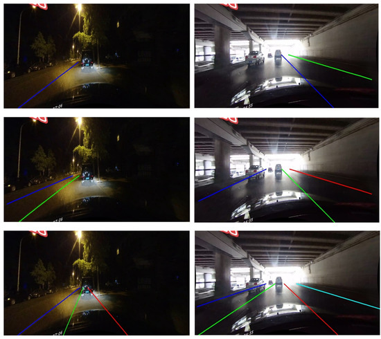
Figure 11. Cases where the lane lines were not fully detected.

5.3. Ablation Experiment

Table 4 illustrates the effectiveness of long-range dependence information in the feature extraction for lane line detection. We compared our proposed model, namely, NLNet, with the state-of-the-art (SOTA) model, namely, CLRNet. However, CLRNet does not fully utilize long-range dependence information, which is a critical factor in achieving high performance. Our NLNet model takes advantage of this information to improve the accuracy and efficiency of lane line detection tasks. The experimental results were conducted using the test data set of Lane Segmentation Using Convolutional Neural Network (CLUane). We selected mF1, F1@50, and F1@75 as the evaluation metrics to observe the detection results. As shown in Table 3, the NLNet model, which effectively utilizes long-range dependence information, outperformed CLRNet in all three evaluation metrics.

Table 4. Ablation experiment. (the bold is to highlight the experimental results of our model which are better than other models.)

Model	Long-Range Dependence	Backbone	mF1	F1@50	F1@75
CLRNet		DLA34	55.64	80.47	62.78
NLNet(ours)	√	DLA34	55.75	80.49	63.16

5.4. Discussion

Lane detection is an essential component of many advanced driver assistance systems (ADAS) and autonomous driving systems, as it provides information about the position and orientation of the vehicle relative to the road and other vehicles. By analyzing the main shortcomings of current lane detection models, the idea of further enhancing long-range dependence and obtaining more global information is absorbed into the optimization and improvement of the lane detection model. The nonlocal module plays an important role in the implementation of this idea scheme and successfully helped us to build a new model, namely, NLNet. NLNet is a new lane detection model based on CLRNet, which works on L2 with DLA34 as the backbone and the nonlocal module for long-range dependency implementation. Results tested on the CULane dataset indicate that NLNet outperformed the current state-of-the-art results. According to the current results of the whole lane detection, the lane detection model still has great room for improvement. Although our proposed model achieved state-of-the-art results, it still fell short of the desired accuracy in certain scenarios, such as 55.03 in the no-line scenario and 74.14 in the curve scenario. Going forward, we will prioritize improving the accuracy in these low-performing scenes to enhance the overall performance of the detection system. We believe that there are improvement measures that can be made in the following three aspects: First, the nonlocal module can be applied to the backbone to continue to enhance the long-range dependence. Second, in this study, we still used the loss function in CLRNet, and future refinement of the loss function will also be a future research direction. Third, due to the fact that our proposed NLNet model adds a nonlocal module compared with CLRNet, which increases the complexity of the model, it can be predicted that the inference speed of NLNet will be slower than that of CLRNet. The experimental results also confirmed this. Frames per second (FPS) was used to measure the real-time performance of a model. From Table 3, we can see that the FPS of CLRnet was 94, while the FPS of the NLNet model was 83, which is lower than CLRnet. Other model inference speeds are also shown in Table 3. It is particularly noteworthy that the experimental environment used to calculate the inference speed of all these models was one NVIDIA 1080Ti GPU, and the tests were performed on the same machine. Therefore, improving the detection accuracy without significantly sacrificing inference speed will be one of the key research directions in the next step. In addition, from the data in Table 3, we can observe that the accuracy of lane line detection was not high in the crowded, dazzle, and shadow scenarios. In the crowded and dazzle scenarios, the accuracy of the lane line detection did not exceed 80%, and an accuracy below 80% is obviously very dangerous for driving safety. Therefore, the next research direction will also focus on improving the detection accuracy in these difficult scenarios.

6. Conclusions

Long-range dependence information refers to the relationship between two or more pixels in an image that extends beyond their visual appearance. It is a measure of how dependent a pixel is on its neighbors in terms of color, texture, and spatial arrangement. Understanding the long-range dependence information of an image can significantly enhance the accuracy and efficiency of these tasks. In this study, first, we discovered that CLRNet has not fully utilized the contribution of other global regions (e.g., faraway pixels) to the current region. Second, therefore, we proposed our NLNet model by adding the nonlocal module after noticing that CLRNet does not make full use of the global regions’ contribution. Based on the analysis of the feature map size of each layer of the FPN in CLRNet, we creatively applied the nonlocal module directly to the L2 layer of the FPN to enhance the information about long-range dependence. Finally, test experiments were performed and the test results demonstrated the effectiveness of the long-range dependence information in improving lane line detection performance, and our proposed NLNet model achieved state-of-the-art accuracy on the CULane dataset. In terms of the next research direction, we believe that it should include further enhancement of long-range dependence, optimization of the loss function, acceleration of the inference speed, and effective improvement of the accuracy in difficult scenarios.

References

- Russakovsky, J.; Deng, H.; Su, J.; Krause, S.; Satheesh, S.; Ma, Z.; Huang, A.; Karpathy, A.; Khosla, M.; Bernstein, A.; et al. ImageNet Large Scale Visual Recognition Challenge. Int. J. Comput. Vis. 2015, 5, 211–252. [Google Scholar] [CrossRef]
- Bar Hillel, A.; Lerner, R.; Levi, D.; Raz, G. Recent progress in road and lane detection: A survey. Mach. Vis. Appl. 2012, 25, 727–745. [Google Scholar] [CrossRef]
- Son, J.; Yoo, H.; Kim, S.; Sohn, K. Real-time illumination invariant lane detection for lane departure warning system. Expert Syst. Appl. 2015, 42, 1816–1824. [Google Scholar] [CrossRef]
- Fritsch, J.; Kuhnl, T.; Geiger, A. A new performance measure and evaluation benchmark for road detection algorithms. In Proceedings of the Intelligent Transportation Systems-(ITSC), 2013 16th International IEEE Conference, The Hague, The Netherlands, 6–9 October 2013; pp. 1693–1700. [Google Scholar]
- Aly, M. Real time detection of lane markers in urban streets. In Proceedings of the Intelligent Vehicles Symposium, Eindhoven, Netherlands, 4–6 June 2008; pp. 7–12. [Google Scholar]
- Zheng, T.; Huang, Y.; Liu, Y.; Tang, W.; Yang, Z.; Cai, D.; He, X. CLRNet: Cross Layer Refinement Network for Lane Detection. In Proceedings of the IEEE/CVF Conference on Computer Vision and Pattern Recognition, New Orleans, LA, USA, 19–20 June 2022. [Google Scholar]
- Wang, X.; Girshick, R.; Gupta, A.; He, K. Non-local Neural Networks. arXiv 2018, arXiv:1711.07971. [Google Scholar]
- Lin, T.-Y.; Dollar, P.; Girshick, R.; He, K.; Hariharan, B.; Belongie, S. Feature pyramid networks for object detection. In Proceedings of the IEEE Conference on Computer Vision and Pattern Recognition, Honolulu, HI, USA, 21–26 July 2017; pp. 2117–2125. [Google Scholar]
- Pan, X.; Shi, J.; Luo, P.; Wang, X.; Tang, X. Spatial as deep: Spatial cnn for traffic scene understanding. In Proceedings of the Thirty-Second AAAI Conference on Artificial Intelligence, New Orleans, LA, USA, 2–7 February 2018. [Google Scholar]
- He, K.; Zhang, X.; Ren, S.; Sun, J. Deep Residual Learning for Image Recognition. In Proceedings of the IEEE Conference on Computer Vision and Pattern Recognition (CVPR), Las Vegas, NV, USA, 27–30 June 2016; pp. 770–778. [Google Scholar]
- TuSimple. Tusimple Benchmark. Available online: https://github.com/TuSimple/tusimple-benchmark/ (accessed on 30 September 2020).
- Zheng, T.; Fang, H.; Zhang, Y.; Tang, W.; Yang, Z.; Liu, H.; Cai, D. Resa: Recurrent feature-shift aggregator for lane detection. In Proceedings of the AAAI Conference on Artificial Intelligence, Virtual, 2–9 February 2021; Volume 35, pp. 3547–3554. [Google Scholar]
- Philion, J. Fastdraw: Addressing the long tail of lane detection by adapting a sequential prediction network. In Proceedings of the IEEE/CVF Conference on Computer Vision and Pattern Recognition, Long Beach, CA, USA, 15–20 June 2019; pp. 11582–11591. [Google Scholar]
- Yoo, S.; Lee, H.S.; Myeong, H.; Yun, S.; Park, H.; Cho, J.; Kim, D.H. End-to-end lane marker detection via row-wise classification. In Proceedings of the IEEE/CVF Conference on Computer Vision and Pattern Recognition Workshops, Seattle, WA, USA, 14–19 June 2020; pp. 1006–1007. [Google Scholar]
- Qin, Z.; Wang, H.; Li, X. Ultrafast structure aware deep lane detection. In Proceedings of the Computer Vision–ECCV 2020: 16th European Conference, Glasgow, UK, 23–28 August 2020; Springer: Berlin/Heidelberg, Germany, 2020. Part XXIV 16. pp. 276–291. [Google Scholar]
- Ko, Y.; Lee, Y.; Azam, S.; Munir, F.; Jeon, M.; Pedrycz, W. Key points estimation and point instance segmentation approach for lane detection. IEEE Trans. Intell. Transp. Syst. 2021, 23, 8949–8958. [Google Scholar] [CrossRef]
- Tabelini, L.; Berriel, R.; Paixao, T.M.; Badue, C.; De Souza, A.F.; Oliveira-Santos, T. Keep your eyes on the lane: Real-time attention-guided lane detection. In Proceedings of the IEEE/CVF Conference on Computer Vision and Pattern Recognition, Nashville, TN, USA, 20–25 June 2021; pp. 294–302. [Google Scholar]
- Abualsaud, H.; Liu, S.; Lu, D.; Situ, K.; Rangesh, A.; Trivedi, M.M. Laneaf: Robust multi-lane detection with affinity fields. arXiv 2021, arXiv:2103.12040. [Google Scholar] [CrossRef]
- Su, J.; Chen, C.; Zhang, K.; Luo, J.; Wei, X.; Wei, X. Structure guided lane detection. arXiv 2021, arXiv:2105.05403. [Google Scholar]
- Qu, Z.; Jin, H.; Zhou, Y.; Yang, Z.; Zhang, W. Focus on local: Detecting lane marker from bottom up via key point. In Proceedings of the IEEE/CVF Conference on Computer Vision and Pattern Recognition, Nashville, TN, USA, 20–25 June 2021; pp. 14122–14130. [Google Scholar]
- Liu, L.; Chen, X.; Zhu, S.; Tan, P. Condlanenet: A top-to-down lane detection framework based on conditional convolution. arXiv 2021, arXiv:2105.05003. [Google Scholar]
- Ke, Z.; Junchen, B.; Haidong, S.; Jiabei, H. Federated multi-source domain adversarial adaptation framework for machinery fault diagnosis with data privacy. Reliab. Eng. Syst. Saf. 2023, 236, 109246. [Google Scholar] [CrossRef]
- Ke, Z.; Feng, J.; Haidong, S. A novel conditional weighting transfer Wasserstein auto-encoder for rolling bearing fault diagnosis with multi-source domains. Knowl.-Based Syst. 2023, 262, 110203. [Google Scholar] [CrossRef]
- Zhou, X.; Zhang, L. SA-FPN: An effective feature pyramid network for crowded human detection. Appl. Intell. 2022, 52, 12556–12568. [Google Scholar] [CrossRef]
- Wang, F.; Wang, H.; Zhou, X.; Fu, R. A Driving Fatigue Feature Detection Method Based on Multifractal Theory. IEEE Sens. J. 2022, 22, 19046–19059. [Google Scholar] [CrossRef]
- Xu, J.; Pan, S.; Sun, P.Z.H.; Park, S.H.; Guo, K. Human-Factors-in-Driving-Loop: Driver Identification and Verification via a Deep Learning Approach using Psychological Behavioral Data. IEEE Trans. Intell. Transp. Syst. (IEEE-TITS) 2022, 24, 3383–3394. [Google Scholar] [CrossRef]
- Jin, B.; Vai, M.I. An adaptive ultrasonic backscattered signal processing technique for instantaneous characteristic frequency detection. Bio-Med. Mater. Eng. 2014, 24, 2761–2770. [Google Scholar] [CrossRef] [PubMed]
- Krizhevsky, A.; Sutskever, I.; Hinton, G.E. Imagenet classification with deep convolutional neural networks. Commun. ACM 2017, 60, 84–90. [Google Scholar] [CrossRef]
- Fawcett, T. An introduction to ROC analysis. Pattern Recognit. Lett. 2006, 27, 861–874. [Google Scholar] [CrossRef]
- Liu, S.; Huang, S.; Xu, X.; Lloret, J.; Muhammad, K. Visual Tracking Based on Fuzzy Inference for Intelligent Transportation Systems. IEEE Trans. Intell. Transp. Syst. 2023, ahead of print. [Google Scholar] [CrossRef]
Disclaimer/Publisher’s Note: The statements, opinions and data contained in all publications are solely those of the individual author(s) and contributor(s) and not of MDPI and/or the editor(s). MDPI and/or the editor(s) disclaim responsibility for any injury to people or property resulting from any ideas, methods, instructions or products referred to in the content. |
© 2023 by the authors. Licensee MDPI, Basel, Switzerland. This article is an open access article distributed under the terms and conditions of the Creative Commons Attribution (CC BY) license (https://creativecommons.org/licenses/by/4.0/).