A Feedrate Planning Method in CNC System Based on Servo Response Error Model

Abstract

Reducing servo response error and further making reduction on contour error is crucial for high-precision computer numerical control (CNC) machine tools. For a permanent magnet synchronous motor (PMSM) servo system, there is always a response lag in feedrate tracking, which would introduce response error into the machining trajectory. Therefore, it is necessary to improve the performance of feedrate planning and interpolation for trajectory path. In this paper, a novel contour error compensation strategy is proposed. Compared with the mainstream methods, the proposed method offers a simplified alternative to existing contour error estimation techniques. Through a three-closed-loop control structure of a PMSM servo system, a response error model is founded. Afterwards, an improved S-model feedrate planning method is introduced according to the servo response error compensation. This predicted error is subsequently compensated in each interpolation cycle, resulting in a reduction of contour error. Finally, simulations and experiments are performed to demonstrate that the contour error can be reduced in both the ‘∞’-shaped Non-Uniform Rational B-Spline (NURBS) curve path and the butterfly-shaped NURBS curve path using the proposed method.

1. Introduction

With the rapid development of industrial and societal progress, high-precision computer numerical control (CNC) machining has become increasingly important in various automation fields [1]. Interpolation of parametric curves is one of the most effective technical solutions in CNC machining. Complex trajectories are expressed as parametric equations, and through feedrate scheduling, interpolation points are calculated in real time, which makes the machining process more intuitive [2,3].

In the process of CNC parametric curve machining, it is essential to select a suitable feedrate planning algorithm before interpolation to enhance machining accuracy. Currently, the commonly used methods for acceleration/deceleration in feedrate planning are linear, exponential, and S-model. The S-model feedrate planning method can ensure a continuous acceleration thus avoiding impacts and vibrations during the machining process. This ensures the trajectory accuracy and reduces loss on the actuating device [4]. In [5], an S-model feedrate planning algorithm considering the constraint of jerk is proposed. However, it does not consider enough kinematic constraints, resulting in limited machining accuracy and efficiency. In [6], an improved S-model feedrate planning algorithm is proposed based on characteristic points. By defining limiting conditions for the axial velocity, acceleration, and jerk of the characteristic points obtained by filtering the chord error. This method can effectively ensure the accuracy of chord error during machining. However, since the continuity of acceleration was not taken into account during feedrate planning, mechanical vibrations of the machine tool still occurred, leading to decreased accuracy. In [7], an S-model feedrate planning algorithm with continuous jerk is proposed, which utilizes sine curves to describe the variation of jerk, and trapezoid curves are employed in [8]. These algorithms enable more precise and efficient machining.

The Servo system serves as the actuating device in CNC machine tools. The primary purpose is to effectively track the pre-scheduled feedrate profile in real-time while ensuring the tool precisely track along the desired trajectory. Contour error is defined as the distance between the actual tool position and the planned trajectory. It is mainly caused by servo dynamics, thermal strains, data losses and other external disturbances, etc. [9]. A typical servo system consists of three feedback loops, which are current-, speed- and position-loop. The inherent characteristic of a physical system is that its response consistently exhibits a delay relative to its execution. Consequently, for a closed-loop servo system, the response lag in the dynamic process would bring response error into the machining trajectory. If not appropriately compensated, contour errors can cause severe deviations in the machine tool trajectory and even lead to workpieces failures.

Different control methods are developed and proposed to reduce contour error and to enhance machining precision. Servo controller optimization is one of the most important solutions for contour error reduction. In [10], a cross-coupled controller (CCC) is proposed to attenuate the dynamic response error in linear and circular trajectories. Through estimating the response error of a single-axis servo system, the CNC contour error is decoupled and compensated by regulating each axis. In [11,12], an improved contour error estimation method is proposed, and the CCC controller is extended to arbitrary trajectories. The contour error is approximated as the projection of the tracking error onto the normal direction of the reference point. In [13,14], the CCC method is further extended to three-dimensional systems. A zero-phase error tracking controller (ZPETC) is proposed to reduce the tracking error of each axis through pole/zero pair elimination [15]. In [16], ZPETC and PID are combined to suppress motor disturbances for better feedrate tracking. Some other kinds of controllers, such as model predictive control, multilevel fuzzy control, sliding mode control, etc. are also investigated to improve the CNC contouring performance [17,18,19]. These methods can be categorized as contour error closed-loop schemes, where the contour error is compensated in real-time machining with self-adaptive controllers or nonlinear high-performance controllers. As to machining error modelling and estimation, the CNC machine is mostly considered as a whole entity. However, the machine tool behaviour depends on servo dynamics of all axis. Investigating each servo’s performance maintains the estimated machining error’s precision.

Another contour error reduction solution is changing feedrate constraints based on the contour error modelling before feedrate scheduling. To compensate for the servo responses error, a first-order contour error model of the servo system is built [20] and new constraints are determined to refine the feedrate profile. In [21,22], a second-order contour error model is established for investigation and feedrate constraints determination. In [23], a lag synchronization-based contour error model is developed and utilized to optimize the feedrate constraint. In [24], an adaptive feedrate scheduling method is developed to improve contour precision according to specified constraints. In [25], a novel feedrate scheduling method is proposed constrained by contour error, axis acceleration, jitter, and chord error. These methods can be categorized as contour error open-loop schemes, and contour error is not estimated and compensated in real-time machining. It is investigated only for constraint determination in feedrate scheduling, but in each interpolation period during machining, contour error can hardly be eliminated even with precise estimating results. As to contour error modelling, the CNC machine is usually considered as a cohesive entity, and the machine tool is represented as a first or second-order system. Nevertheless, machine tool behaviour depends on servo dynamics of all axes, whose characteristics relate to damping ratio, overshoot, setting time, rising/falling time etc. Therefore, a more precise depiction of the machine’s behavior becomes imperative to capture its true capabilities effectively.

Accurate contour error modelling and estimation are the foundation of high-precision CNC machining. Furthermore, contour error closed-loop control is also necessary for precision improvement. This paper proposes a servo response error compensation method. A three-closed-loop control structure of a PMSM servo system is established with Proportional-Integral (PI) regulators. According to the control diagram, the servo response transfer function of each axis is derived, and the servo response error model is founded. Then an optimized real-time feedrate refining method is proposed. Based on the pre-scheduled S-model feedrate profile, the response error of each axis can be calculated in every interpolation cycle. Afterwards, the feedrate compensation value is calculated and added to the pre-scheduled feedrate profile to compensate the contour error. After a few interpolation cycles, the contour error of the machining trajectory can be reduced to a lower level, and the machining trajectory precision is finally improved. The main contributions of this paper are listed as follows:

• A servo response error model for each axis is established by utilizing a three-closed-loop control diagram. By calculating and compensating the response error in each interpolation cycle, the contour error induced by response lag can be bounded from the source.
• An enhanced S-model feedrate planning method has been developed, focusing on refining the pre-scheduled tool feedrate. The calculated error in each interpolation cycle based on the servo response error model will be turned into the feedrate constraints for scheduling and finally improve trajectory precision.

The rest of this paper is organized as follows: Section 2 illustrates a PMSM servo system and its control method. Section 3 establishes the response error model based on the servo system control diagram. Section 4 provides the contour error compensation strategy based on feedrate refining. Simulation and experimental results in different scenarios are provided in Section 5 and Section 6 draws the conclusions.

2. Servo System Modelling

2.1. PMSM Model

The dynamical equations of the stator voltage of a surface mounted PMSM (SPMSM) in dq-frame can be given by

$$\left\{\begin{array}{c}{u}_{\mathrm{d}}=R_{\mathrm{s}}{i}_{\mathrm{d}}+\frac{\mathrm{d}{\psi }_{\mathrm{d}}}{\mathrm{d}t}-{\omega }_e{\psi }_{\mathrm{q}}\\ u_{\mathrm{q}}=R_{\mathrm{s}}{i}_{\mathrm{q}}+\frac{\mathrm{d}{\psi }_{\mathrm{q}}}{\mathrm{d}t}+{\omega }_e{\psi }_{\mathrm{d}}\end{array}\right.$$

(1)

where $[u_d,u_q]$ are the stator voltages, $[{\psi }_d,{\psi }_q]$ are the stator flux linkage, ${\omega }_e$ is the angular velocity. The expressions of dq-frame flux linkages and the electromagnetic torque can be given by Equations (2) and (3).

$$\left\{\begin{array}{c}\hfill {\psi }_{\mathrm{d}}=L_{\mathrm{d}}{i}_{\mathrm{d}}+{\psi }_{\mathrm{f}}\hfill \\ \hfill {\psi }_{\mathrm{q}}=L_{\mathrm{q}}{i}_{\mathrm{q}}\hfill \end{array}\right.$$

(2)

$$T_e=\frac{3}{2}p{\psi }_f{i}_q$$

(3)

where $L_d$ and $L_q$ are the d-axis and q-axis stator inductances, ${\psi }_f$ is the rotor permanent magnet flux linkage, $T_e$ is the electromagnetic torque and p is the number of pole pairs.

The mechanical motion equation of a SPMSM can be expressed as Equation (4), where J is the rotational inertia, $T_L$ is the load torque and ${\omega }_m$ is the mechanical angular velocity.

$$J\frac{d{\omega }_r}{dt}=T_e-B{\omega }_m-T_L$$

(4)

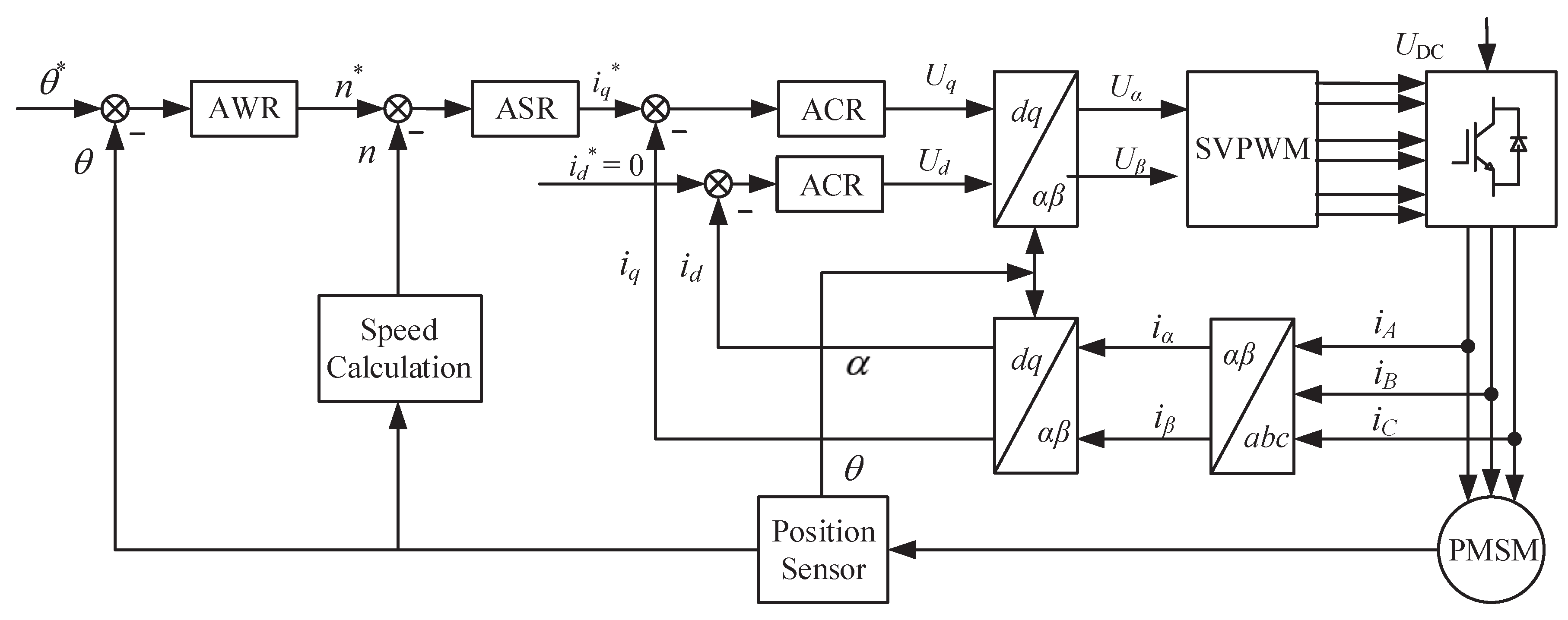
2.2. Modelling of PMSM Servo System

Based on the PMSM model in dq-frame above, the structure for three-closed-loop control of PMSM servo system is displayed in Figure 1. The control strategy is based on space vector pulse width modulation (SVPWM) control with $i_d^{*}=0$.

In this paper, a control scheme is introduced that utilizes two PI regulators in the current-loop to control $i_d$ and $i_q$ respectively. Additionally, a PI regulator is implemented in the speed-loop to effectively counteract disturbances. The inverter link can be considered as a first-order inertia link with a time constant. Then, a block diagram of the servo system can be obtained, as shown in Figure 2. $K_T$ is the torque coefficient of the motor, $T_m$ is the mechanical time constant of the motor, and $K_e$ is the counter-electromotive force coefficient of the PMSM.

In order to guarantee the accuracy and the following performance of the system, the typical type I system is used for the current-loop designing and the typical type II system is used for the speed-loop. Afterwards, the position-loop control structure diagram can be obtained, as shown in Figure 3.

Only P control is employed in the position-loop to avoid overshoot, and the proportional coefficient is $K_{\theta }$. By denoting the unit step response time of the servo system as the speed-loop time constant of the equivalent inertial link $T_v$, $T_v=nJ/9.55T_e$ can be obtained from the equations of kinematics, and $K_v$ is the speed closed-loop gain which can be acquired according to the closed-loop transfer function of speed-loop. And then, utilizing the typical type I system law, the closed-loop transfer function of the position-loop can be expressed as

$$G_{p\left(s\right)}=\frac{G_{opp\left(s\right)}}{1+G_{opp\left(s\right)}}=\frac{K/T_v}{s^2+s/T_v+K/T_v}$$

(5)

where the open-loop gain of the position-loop $K=K_{\theta }$$K_v$, and in order to get a Critically Damped System, $K=0.25/T_v$ can be obtained.

3. Servo Response Error Analysis and Solving

During the machining process, response errors can occur in CNC machines as a result of the response lag inherent in the servo system. For using the sampled-data method, theoretically, there is a ramp signal $X\left(T\right)=VT$ approximating the ideal curve trajectory through a straight line segment in each interpolation cycle. Figure 4 shows the tracking error by inputting a constant feedrate in an interpolation cycle. As is shown in Figure 4, when the time is $T_i+1$, the actual value can track the ideal value at the time of $T_i$. Therefore, there is always an error $\Delta$E between the actual and the ideal trajectory when the system has reached the given feedrate and entered the steady state.

Servo response error modelling is crucial in reducing the impact of such errors on machining trajectories. By accurately modelling the response error, it becomes possible to understand its characteristics and quantify its influence on the machining process. This information is essential for developing effective compensation techniques and control strategies to mitigate the adverse effects of response errors.

Define a unit ramp signal $r\left(t\right)=t$ as the input signal at each interpolation cycle, the output of a typical second-order system can be derived as

$$\begin{array}{cc}\hfill C\left(s\right)& =\frac{{\omega }_n^2}{s^2(s^2+2\xi {\omega }_{n}s+{\omega }_n^2)}\hfill \\ & \hfill =\frac{1}{s^2}-\frac{2\xi /{\omega }_n}{s}+\frac{2\xi /{\omega }_n(s+\xi {\omega }_n)+(2{\xi }^2-1)}{s^2+2\xi {\omega }_{n}s+{\omega }_n^2}\hfill \end{array}$$

(6)

Taking the Inverse Laplace Transformation (ILT) of Equation (6), the unit ramp response at $\xi =1$ can be obtained.

$$c\left(t\right)=t-\frac{2}{{\omega }_n}+\frac{2}{{\omega }_n}(1+\frac{1}{2}{\omega }_{n}t)e^{-{\omega }_{n}t},t\ge 0$$

(7)

As shown in Figure 5, the response of a second-order system is $C\left(t\right)$, when the input is a unit ramp signal $r\left(t\right)=t$, and the steady-state error value is $2/{\omega }_n$. The transient component of the ramp response is an aperiodic damping function.

According to Equation (7), the error response function is derived as

$$e\left(t\right)=\frac{2}{{\omega }_n}[1-(1+\frac{1}{2}{\omega }_{n}t)e^{-{\omega }_{n}t}],t\ge 0$$

(8)

In accordance with the PMSM model and the designed controller, the closed-loop transfer function Equation (5) can be effectively represented as a typical second-order system. In the trajectory interpolation process, the input to the system for each interpolation cycle is a ramp signal $r\left(t\right)=V_{i}t$, where $V_i$ is the feedrate of the single axis for that cycle. At this point, the ramp response can be derive as Equation (9), and then the error response can be obtained as Equation (10).

$$c\left(t\right)=v_i(t-2\sqrt{\frac{T_v}{K}}+2\sqrt{\frac{T_v}{K}}(1+\frac{1}{2}\sqrt{\frac{K}{T_v}}t)e^{-\sqrt{\frac{K}{T_v}}t}),t\ge 0$$

(9)

$$e\left(t\right)=v_i(2\sqrt{\frac{T_v}{K}}[1-(1+\frac{1}{2}\sqrt{\frac{K}{T_v}}t)e^{-\sqrt{\frac{K}{T_v}}t}]),t\ge 0$$

(10)

Utilizing the final-value theory, the steady-state error can be derived as

$$e_{ss}=\underset{t\to \infty }{lim}e\left(t\right)=2\sqrt{\frac{T_v}{K}}{v}_{ix}$$

(11)

When the interpolation period is $T_s$, the servo response error of the single-axis (e.g., x-axis) can be obtained as

$$E_i=\left\{\begin{array}{c}\hfill v_{ix}(2\sqrt{\frac{T_v}{K}}[1-(1+\frac{1}{2}\sqrt{\frac{K}{T_v}}{T}_s)e^{-\sqrt{\frac{K}{T_v}}{T}_s}]),T_s>t_s\hfill \\ 2\sqrt{\frac{T_v}{K}}{v}_{ix},T_s<t_s\hfill \end{array}\right.$$

(12)

where $t_s=4.1/(K/T_v)$ is the regulation time of the error response.

According to the above analysis, the servo response error relates to the position-loop gain, interpolation period, and feedrate. When the interpolation period $T_s$ is predefined, the larger the position-loop gain K, the smaller the servo response error. To ensure system stability, manageable position-loop gain is essential. Therefore, feedrate planning is the only way to reduce the servo response error once the position-loop gain K is determined.

4. Feedrate Planning and Error Compensation

4.1. S-Model Feedrate Planning with Improved Constraints

During trajectory processing, it is vital for the CNC system to operate within its designated parameters to prevent mechanical vibration and maintain accuracy. The effects of various constraints must be considered when doing the feedrate planning.

The maximum allowable chord error ${\delta }_{max}$ determines the maximum allowable feedrate $v_{cc}$ in an interpolation period $T_s$. For a tool path $C\left(u\right)$, the feedrate constraint can be derived as

$$v_{cc}=\frac{2}{T_s}\sqrt{{\rho }_i^2-{({\rho }_i-{\delta }_{max})}^2},{\delta }_0\le {\delta }_{max}$$

(13)

The constraints of the axial velocities $v_{xmax}$, $v_{ymax}$, axial accelerations $a_{xmax}$, $a_{ymax}$, and axial jerks $j_{xmax}$, $j_{ymax}$ can be represented by Equations (14) and (15).

$$\left\{\begin{array}{c}\hfill \left|v_{ix}\right|\le v_{xmax}\hfill \\ \hfill \left|a_{ix}\right|\le a_{xmax}\hfill \\ \hfill \left|j_{ix}\right|\le j_{xmax}\hfill \end{array}\right.$$

(14)

$$\left\{\begin{array}{c}\hfill \left|v_{iy}\right|\le v_{ymax}\hfill \\ \hfill \left|a_{iy}\right|\le a_{ymax}\hfill \\ \hfill \left|j_{iy}\right|\le j_{ymax}\hfill \end{array}\right.$$

(15)

The relationship between the axial parameters and the feedrate is needed, by decomposing the feedrate in the rectangular coordinate system. The relationship between feedrate and axial velocities can be obtained as Equation (16), where $v_i$ is the feedrate and $\alpha$, $\beta$ are the first-order derivative factors, given by Equation (17).

$$\left\{\begin{array}{c}\hfill v_{ix}=\left|v_i\right|·\alpha \hfill \\ \hfill v_{iy}=\left|v_i\right|·\beta \hfill \end{array}\right.$$

(16)

$$\left\{\begin{array}{c}\hfill \alpha =\frac{x^{\prime }\left(u\right)}{\left|C^{\prime }\left(u\right)\right|}\hfill \\ \hfill \beta =\frac{y^{\prime }\left(u\right)}{\left|C^{\prime }\left(u\right)\right|}\hfill \end{array}\right.$$

(17)

Since the axial velocities is limited to $v_{xmax}$ and $v_{ymax}$, according to Equations (16) and (17), the feedrate constraint can be obtained as

$$\left|v_i\right|\le v_{mvxy}=min\{\frac{v_{xmax}}{\left|\alpha \right|},\frac{v_{ymax}}{\left|\beta \right|}\}$$

(18)

In addition, the axial acceleration and the axial jerk limits should be taken into account. The feedrate constraints corresponding to the axial acceleration limit are challenging to obtain by decomposing the axial acceleration directly. However, the constraints on the feedrate and centripetal acceleration need to satisfy Equation (19), and the curve curvature $K_i$ in Equation (19) can be obtained from Equation (20).

$$v_i\le \sqrt{\frac{a_{nmax}}{{\kappa }_i}}$$

(19)

$${\kappa }_i=\frac{∥C^{\prime }\left(u_i\right)\times C^{″}\left(u_i\right)∥}{{∥C^{\prime }\left(u_i\right)∥}^3}$$

(20)

By the coordinate decomposition, the axial accelerations equation Equation (21) is firstly obtained.

$$\left\{\begin{array}{c}\hfill a_{ix}=\left|a_{\tau }\right|·\alpha +\left|a_n\right|·\beta \hfill \\ \hfill a_{iy}=\left|a_{\tau }\right|·\beta -\left|a_n\right|·\alpha \hfill \end{array}\right.$$

(21)

According to the axial limit and the triangle inequality, Equation (22) can be obtained by Equation (21).

$$\left\{\begin{array}{c}\hfill \left|a_{ix}\right|\le \left|a_{\tau }·\alpha \right|+\left|a_n·\beta \right|\le a_{xmax}\hfill \\ \hfill \left|a_{iy}\right|=\left|a_{\tau }·\beta \right|-\left|a_n·\alpha \right|\le a_{ymax}\hfill \end{array}\right.$$

(22)

The limit of an in Equation (22) can be given by Equation (23), where M is the centripetal acceleration coefficient, and is obtained by experiments in [26,27]. It determines the maximum allowed centripetal acceleration, and there should be a positive correlation between the M and the centripetal acceleration.

$$\left\{\begin{array}{c}\hfill \left|a_n·\beta \right|\le M{a}_{xmax}\hfill \\ \hfill \left|a_n·\alpha \right|\le M{a}_{ymax}\hfill \end{array}\right.$$

(23)

Then, according to the relationship between feedrate and centripetal acceleration in Equation (19), the feedrate constraint corresponding to the axial acceleration limit can be obtained as Equation (24). During the feedrate scheduling, the tangential acceleration ${\alpha }_{\tau }$ should always satisfy Equation (22).

$$\left|v_i\right|\le v_{maxy}=min\{\sqrt{\frac{M{a}_{xmax}}{{\kappa }_i\left|\beta \right|}},\sqrt{\frac{M{a}_{ymax}}{{\kappa }_i\left|\alpha \right|}}\}$$

(24)

Similar to the axial acceleration limit, the limit of axial acceleration can be obtained in Equation (25), where $j_{\tau }$, $j_n$ represent the tangential and centripetal jerk, respectively.

$$\left\{\begin{array}{c}\hfill \left|j_{ix}\right|\le \left|j_{\tau }·\alpha \right|+\left|j_n·\beta \right|\le j_{xmax}\hfill \\ \hfill \left|j_{iy}\right|=\left|j_{\tau }·\beta \right|-\left|j_n·\alpha \right|\le j_{ymax}\hfill \end{array}\right.$$

(25)

This paper applies a seven-segment S-model feedrate curve for feedrate scheduling, which includes seven different motion states and enables smooth acceleration change. The jerk in each motion state cycle is defined as a constant allowed by the system. Thus the limit of the jerk is derived as

$$\left\{\begin{array}{c}\hfill \left|j_n·\beta \right|\le j_{xmax}-\left|j_{\tau }·\alpha \right|\hfill \\ \hfill \left|j_n·\alpha \right|\le j_{ymax}-\left|j_{\tau }·\beta \right|\hfill \end{array}\right.$$

(26)

Then, through the relationship between the feedrate and centripetal jerk in Equation (27), the improved constraint is derived as Equation (28).

$$v_i\le \sqrt[3]{\frac{j_{nmax}}{{{\kappa }_i}^2}}$$

(27)

$$\left|v_i\right|\le v_{mjxy}=min\{\sqrt[3]{\frac{j_{xmax}-\left|j_{\tau }·\alpha \right|}{{{\kappa }_i}^2\left|\beta \right|}},\sqrt[3]{\frac{j_{ymax}-\left|j_{\tau }·\beta \right|}{{{\kappa }_i}^2\left|\alpha \right|}}\}$$

(28)

Considering all the above constraints, the total feedrate constraints at any point on the desired trajectory can be expressed as Equation (29). With the improved constraints, the scheduling of the feedrate profile can be more rational, and the actual chord error can be limited below ${\delta }_{max}$.

$$v_i\le min\{v_{mvxy},v_{maxy},v_{mjxy},v_{max},v_{cc}\}$$

(29)

The seven-stage S-model feedrate planning is gradually become one of the most commonly used multi-stage feedrate planning methods in CNC systems due to its simplicity. By applying the improved constraints to this model, a more suitable S-model feedrate curve path can be obtained, and it can enhance the accuracy of the machining trajectory.

4.2. Error Compensation

To reduce the influence of servo response error on contour accuracy, compensation is applied to the servo response error of the two axes (x-axis & y-axis) during each interpolation cycle. The compensation process is depicted in Figure 6.

The process of servo response error compensation can be seen from the figure:

• According to the given parameters, plan the feedrate of curve trajectory with chord error constraints, kinetic constraints and axial parameters constraints;
• Calculate the response error (x-axis & y-axis) in an interpolation period based on the servo response error model and substitute the error for the feedrate constraints to get compensated;
• The two-axis motion is controlled separately through the compensated interpolation information to complete the curve trajectory processing.

Calculating the compensation value is an essential step in the error compensation processes. Define $f\left(\lambda \right)=\lambda E_i$ as the value of the machining trajectory path in a interpolation cycle, where $\lambda$ is the compensation factor, and $E_i$ is the tracking error in that interpolation cycle.

As shown in Figure 7, $v\left(t\right)$ is the feedrate planning curve for a certain interpolation period without compensation, and $v^{\prime }\left(t\right)$ is the improved feedrate planning curve with compensation. Define $\Delta E$ is the maximum compensation ability which can be obtained by the difference of the two curves in an interpolation cycle. If $\Delta E>E_i$, the tracking error can be compensated in an interpolation cycle, then let $\lambda =1$. On the contrary, if $\Delta E<E_i$, the tracking error cannot be fully compensated in one interpolation cycle, then let $\lambda =\Delta E/E_i$. Therefore, the compensation factor $\lambda$ satisfies

$$\lambda =\left\{\begin{array}{cc}1& ,\Delta E>E_i\\ \Delta E/E_i& ,\Delta E<E_i\end{array}\right.$$

(30)

The error in each interpolation cycle will be compensated by the calculated compensation value $f\left(\lambda \right)$. Figure 8 shows the error compensation diagram when $v_s<v_e$ and Figure 9 shows the error compensation diagram when $v_s>v_e$. The actual trajectory length $S_{\left(i\right)}^{*}$ is obtained by compensating for the preset trajectory length $s_{\left(i\right)}$. The relationship between the trajectory length before and after compensation satisfy

$$s_{\left(i\right)}^{*}=\left\{\begin{array}{cc}{s}_{\left(i\right)}-f\left(\lambda \right)& ,v_s>v_e\\ s_{\left(i\right)}+f\left(\lambda \right)& ,v_s<v_e\end{array}\right.$$

(31)

5. Simulation Analysis and Experimental Verification

5.1. Servo Response Error Model Simulation Verification

To verify the CNC machine servo system will generate response lag error during interpolation even the system has good performance, simulations were performed in the MATLAB R2020a/Simulink. The PMSM parameters are listed in

Table 1. System parameters in simulations.

Parameters	Symbols	Values
Rated voltage	$U_N$	24 V
Rated current	$I_N$	3.3 A
Rated power	$P_N$	60 W
Rated speed	$n_N$	3000 r/min
Rated torque	$T_L$	0.18 N·m
Rotor flux	${\phi }_f$	0.1119 Wb
Stator resistance	$R_s$	0.11 $\mathsf{\Omega }$
Direct-axis inductance	$L_d$	0.00129 H
Cross-axis inductance	$L_q$	0.00129 H
Rotational inertia	J	0.0016 Kg·m2
Pole pairs	p	2

.

The simulation waveforms of position and speed are shown in Figure 10. The load torque is changed from 0.18 N·m to 0 N·m at 1 s.

5.2. Experimental Verification

In this section, a CNC platform is built to verify the effectiveness of the error compensation method proposed in this paper. As shown in Figure 11, the CNC platform consists of three main parts: the upper computer unit, the central control unit and the lower computer unit. The upper computer is operated on an Intel(R) Core(TM) i5-8400 CPU @ 2.80 GHz laptop. The central control unit uses the STM32F429 as the core processor and communicates with the upper and the lower computer via RS232 serial communication. The lower computer unit is the PMSM drive system, which controls the parameters of each axis to finish the curve trajectory.

Due to its ability to flexibly control and modify shapes, NURBS curve path have found extensive applications in engineering. Several international standards have defined it as the sole method for representing free-form curves in CNC systems. Therefore, two representative NURBS curves, Butterfly-shaped and ‘∞’-shaped NURBS curve path, are chosen for the comparative experiments. The parameters employed for the tests are illustrated in

Table 2. Feedrate planning parameters.

Parameters	Symbols	Values
Interpolation period	$T_s$	1 ms
Maximum allowed chord error	${\delta }_{\max }$	0.001 mm
Maximum tangential feedrate	$v_{\max }$	100 mm/s
Maximum tangential acceleration	$a_{\max }$	3000 mm/s2
Maximum tangential jerk	$j_{\max }$	60,000 mm/s3
Maximum axial velocities	$v_{x\max },v_{y\max }$	100 mm/s
Maximum axial accelerations	$a_{x\max },a_{y\max }$	3000 mm/s2
Maximum axial jerks	$j_{x\max },j_{y\max }$	60,000 mm/s3
Centripetal acceleration coefficient	M	0.2

, which are artificially set according to the commonly used values.

5.2.1. ‘∞’-Shaped NURBS Curve Path

With the proposed error compensation method, the final curve path is displayed in Figure 12. Curve 1 (coloured blue) represents the ideal ‘∞’ NURBS curve, Curve 2 (coloured green) and Curve 3 (coloured red) represents the compensated curve path and uncompensated curve path, respectively. Figure 12 shows that the proposed method achieves a closer alignment between the machining trajectory and the ideal trajectory curve path.

The maximum and the average value of the contour error before and after the compensation are listed in

Table 3. Error comparison results before and after compensation (’∞-shaped NURBS curve’).

Values before or after Compensation	Maximum Value	Average Value
Before compensation (mm)	0.78	0.24
After compensation (mm)	0.18	0.06
Reduction ratio (%)	69.23%	66.67%

. The maximum value of the contour error has dropped by approximately 69.23% from 0.78 mm to 0.24 mm. The average value of the contour error has reduced by about 66.67% from 0.18 mm to 0.06 mm. The contour error diagram before and after compensation is shown in Figure 13.

5.2.2. Butterfly-Shaped NURBS Curve Path

The final curve path with the error compensation method is shown in Figure 14. The ideal butterfly-shaped NURBS curve is curve 1 (coloured blue), and the machining curve path before and after the servo response error compensation is curve 3 (coloured red) and curve 2 (coloured green). The experiment data is listed in

Table 4. Error comparison results before and after compensation (butterfly-shaped NURBS curve).

Values before or after Compensation	Maximum Value	Average Value
Before compensation (mm)	0.58	0.18
After compensation (mm)	0.30	0.11
Reduction ratio (%)	68.96%	63.51%

. The maximum value of the contour error has dropped by about 68.96% from 0.58 mm to 0.18 mm by using the compensation method. The average value of the contour error has dropped by about 63.51% from 0.30 mm to 0.11 mm. The comparison graph of the contour error before and after compensation is shown in Figure 15.

In comparison the method and results of [3,25], respectively. The method proposed in [3] presents an indirect strategy for compensating contour errors. Instead of directly estimating the contour error, it employs iterative calculation of the chord error to estimate the contour error in real-time. The experimental results demonstrate that this method achieves a reduction of approximately 70% in contour error under both data loss and external disturbance scenarios. However, the method does not address the issue of servo dynamic error. This paper focuses on the contour error induced by servo response lag and provides a direct compensation method, which is easier to implement. The achieved reduction in contour error aligns with [3].

According to the findings presented in [25], the contour error can be reduced by 55% for the butterfly-shaped curve. In comparison, this paper demonstrates a more significant reduction of over 63% in both the ‘∞’-shaped and butterfly-shaped curves, more effective.

6. Conclusions

In this paper, a novel contour error compensation strategy is proposed to reduce the contour error resulting from servo response lag in CNC machining. By utilizing a servo response error model, the contour error can be reduced from the source. A response error model is developed based on the mathematical model of the two-axis servo motion control system, establishing the relationship between feedrate and servo response error during each interpolation cycle. Additionally, an improved feedrate planning algorithm is also proposed based on the improved feedrate constraints, which can compensate for the response error in real-time according to the error model.

In order to validate the proposed method, several comparative experiments are conducted. The results show that the maximum contour error is reduced by about 69.23% and the overall contour error is reduced by about 66.67% for the ‘∞’-shaped NURBS curve path after compensation compared with that before; the maximum contour error is reduced by about 68.96% and the overall contour error is dropped by about 63.51% for the butterfly-shaped NURBS curve path with the servo response error compensation. All results validate the effectiveness of the proposed response error compensation method in reducing contour errors during CNC machining.

References

1. Chen, L.; Khong, H.; Hsieh, S. Contouring control of a five-axis machine tool with equivalent errors. Electronics 2022, 11, 2521. [Google Scholar] [CrossRef]
2. Lin, F.; Shen, L.; Mi, Z. Certified space curve fitting and trajectory planning for CNC machining with cubic B-splines. Comput. Aided Des. 2019, 106, 13–29. [Google Scholar] [CrossRef]
3. Liu, B.; Xu, M.; Fang, J. A feedrate optimization method for CNC machining based on chord error revaluation and contour error reduction. Int. J. Adv. Manuf. Technol. 2020, 111, 3437–3452. [Google Scholar] [CrossRef]
4. Liu, Z.; Dong, J.; Ding, Y. The study of S-shaped acceleration and deceleration curve and the trajectory planning strategy analysis. Key Eng. Mater. 2016, 693, 1195–1199. [Google Scholar] [CrossRef]
5. Erkorkmaz, K.; Altintas, Y. High speed CNC system design. Part I: Jerk limited trajectory generation and quintic spline interpolation. Int. J. Mach. Tools Manuf. 2001, 41, 1323–1345. [Google Scholar] [CrossRef]
6. Cheng, C.; Tsai, M. Real-time variable feed rate NURBS curve interpolator for CNC machining. Int. J. Adv. Manuf. Technol. 2004, 23, 865–873. [Google Scholar] [CrossRef]
7. Fan, W.; Gao, X.; Yan, W. Interpolation of parametric CNC machining path under confined jounce. Int. J. Adv. Manuf. Technol. 2012, 62, 719–739. [Google Scholar] [CrossRef]
8. Huang, J.; Zhu, L. Feedrate scheduling for interpolation of parametric tool path using the sine series representation of jerk profile. Proc. Inst. Mech. Eng. B J. Eng. Manuf. 2017, 231, 2359–2371. [Google Scholar] [CrossRef]
9. Erwinski, K.; Paprocki, M.; Wawrzak, A. Neural network contour error predictor in CNC control systems. In Proceedings of the 2016 21st International Conference on Methods and Models in Automation and Robotics (MMAR), Miedzyzdroje, Poland, 29 August–1 September 2016. [Google Scholar] [CrossRef]
10. Koren, Y. Cross-coupled biaxial computer control for manufacturing systems. J. Dyn. Syst. Meas. Control. 1980, 102, 265–272. [Google Scholar] [CrossRef]
11. Yeh, S.; Hsu, P. Estimation of the contouring error vector for the cross-coupled control design. IEEE/ASME Trans. Mechatron. 2002, 7, 44–51. [Google Scholar] [CrossRef] [Green Version]
12. Liu, Z.; Dong, J.; Wang, T. Real-time exact contour error calculation of NURBS tool path for contour control. Int. J. Adv. Manuf. Technol. 2020, 108, 2803–2821. [Google Scholar] [CrossRef]
13. Zhang, D.; Yang, J.; Chen, Y. A two-layered cross coupling control scheme for a three-dimensional motion control system. Int. J. Mach. Tools Manuf. 2015, 98, 12–20. [Google Scholar] [CrossRef]
14. Liu, W.; Ren, F.; Sun, Y. Contour error pre-compensation for three-axis machine tools by using cross-coupled dynamic friction control. Int. J. Adv. Manuf. Technol. 2018, 98, 551–563. [Google Scholar] [CrossRef]
15. Tsao, T.; Tomizuka, M. Adaptive Zero Phase Error Tracking Algorithm for Digital Control. ASME J. Dyn. Syst. Meas. Control 1987, 109, 349–354. [Google Scholar] [CrossRef]
16. Tsao, T.; Tsao Tomizuka, M. Adaptive And Repetitive Digital Control Algorithms for Noncircular Machining. In Proceedings of the 1988 American Control Conference, Atlanta, GA, USA, 15–17 June 1988. [Google Scholar] [CrossRef]
17. Lam, D.; Manzie, C.; Good, M. Model Predictive Contouring Control for Biaxial Systems. IEEE Trans. Control. Syst. Technol. 2013, 21, 552–559. [Google Scholar] [CrossRef]
18. Ngo, P.; Shin, Y. Milling contour error control using multilevel fuzzy controller. Int. J. Adv. Manuf. Technol. 2013, 66, 1641–1655. [Google Scholar] [CrossRef]
19. Mao, W.; Shiu, D. Precision Trajectory Tracking on XY Motion Stage Using Robust Interval Type-2 Fuzzy PI Sliding Mode Control Method. Int. J. Precis. Eng. Manuf. 2020, 21, 797–818. [Google Scholar] [CrossRef]
20. Chen, M.; Sun, Y. A moving knot sequence-based feedrate scheduling method of parametric interpolator for CNC machining with contour error and drive constraints. Int. J. Adv. Manuf. Technol. 2018, 98, 487–504. [Google Scholar] [CrossRef]
21. Jia, Z.; Song, D.; Ma, J.; Hu, G. A NURBS interpolator with constant speed at feedrate-sensitive regions under drive and contour-error constraints. Int. J. Mach. Tools Manuf. 2017, 116, 1–17. [Google Scholar] [CrossRef]
22. Dong, J.; Li, B.; Ding, Y. Smooth feedrate planning for continuous short line tool path with contour error constraint. Int. J. Mach. Tools Manuf. 2014, 76, 1–12. [Google Scholar] [CrossRef]
23. Wang, J.; Sui, Z.; Tian, Y. A speed optimization algorithm based on the contour error model of lag synchronization for CNC cam grinding. Int. J. Adv. Manuf. Technol. 2015, 80, 1421–1432. [Google Scholar] [CrossRef]
24. Li, J.; Huang, D.; Li, Y. Contour Error Compensation based on Feed Rate Adjustment. In Proceedings of the 2021 IEEE 16th Conference on Industrial Electronics and Applications (ICIEA), Chengdu, China, 1–4 August 2021. [Google Scholar] [CrossRef]
25. Chen, M.; Xu, J.; Sun, Y. Adaptive feedrate planning for continuous parametric tool path with confined contour error and axis jerks. Int. J. Adv. Manuf. Technol. 2017, 89, 1113–1125. [Google Scholar] [CrossRef]
26. Li, J.; Liu, Y.; Li, Y. S-model speed planning of NURBS curve based on uniaxial performance limitation. IEEE Access 2019, 7, 60837–60849. [Google Scholar] [CrossRef]
27. Zhong, W.; Luo, X.; Chang, W. A real-time interpolator for parametric curves. Int. J. Mach. Tools Manuf. 2020, 125, 133–145. [Google Scholar] [CrossRef] [Green Version]
Figure 1. General structure of three-closed-loop control in servo system.
Electronics 12 03150 g001
Figure 2. Servo system structure block diagram.
Electronics 12 03150 g002
Figure 3. Position-loop structure block diagram.
Electronics 12 03150 g003
Figure 4. Tracking error under constant feedrate input of an interpolation cycle.
Electronics 12 03150 g004
Figure 5. Unit slope response curve of second-order system.
Electronics 12 03150 g005
Figure 6. The flowchart of the proposed error compensation method.
Electronics 12 03150 g006
Figure 7. Feedrate planning curve for a certain interpolation cycle.
Electronics 12 03150 g007
Figure 8. Error compensation diagram at v s < v e .
Electronics 12 03150 g008
Figure 9. Error compensation diagram at v s > v e .
Electronics 12 03150 g009
Figure 10. Slope response simulation diagram. (a) Position. (b) Speed.
Electronics 12 03150 g010
Figure 11. Schematic diagram of the experimental platform.
Electronics 12 03150 g011
Figure 12. ‘∞’-shaped NURBS curve trajectory without and with error compensation.
Electronics 12 03150 g012
Figure 13. Contour error diagram before and after error compensation.
Electronics 12 03150 g013
Figure 14. Comparison of butterfly-shaped NURBS curve machining paths before and after error compensation.
Electronics 12 03150 g014
Figure 15. Contour error diagram before and after error compensation.
Electronics 12 03150 g015