Abstract
A LiDAR sensor is a valuable tool for environmental perception as it can generate 3D point cloud data with reflectivity and position information by reflecting laser beams. However, it cannot provide the meaning of each point cloud cluster, so many studies focus on identifying semantic information about point clouds. This paper explores point cloud segmentation and presents a lightweight convolutional network called Fast Context-Awareness Encoder (FCAE), which can obtain semantic information about the point cloud cluster at different levels. The surrounding features of points are extracted as local features through the local context awareness network, then combined with global features, which are highly abstracted from the local features, to obtain more accurate semantic segmentation of the discrete points in space. The proposed algorithm has been compared and verified against other semantic KITTI data algorithms and has achieved state-of-the-art performance. Due to its ability to note fine-grained features on the z-axis in space, the algorithm shows higher prediction accuracy for certain types of objects. Moreover, the training and validation time is short, and the algorithm can meet high real-time requirements for 3D perception tasks.
1. Introduction
Environmental perception is the most challenging task for an autonomous driving system to analyze real-time data and provide a reliable driving recommendation. With the advent of the Internet of Things (IoT), several automated driving technologies utilize the LiDAR sensor or depth cameras to acquire rich environmental information and get 3D data of the surrounding objects [1].
Typically, the approach for perceiving point cloud data from LiDAR involves object detection and point cloud segmentation. While 3D target detection provides an approximate estimation of the point cloud, the 3D point cloud semantic segmentation function [2] classifies each point of the scene point cloud individually and allows for fine differentiation of point clouds. This paper focuses on exploring point cloud segmentation methods to obtain more accurate semantic information.
Most of the algorithms used for 3D object detection and segmentation are based either on voxel or point features. Point-level feature algorithms such as Pointnet [3] do not pay much attention to the surrounding point clouds, leading to insufficient accuracy. Pointnet++ [4] improves the features of surrounding point clouds using multi-scale grouping, but this approach requires large and intensive computations. Voxel-based algorithms such as Voxelnet [5] directly voxelate the point cloud, missing out on the fine-grained features of points. Point Pillars [6] and other algorithms transform 3D data into a pseudo-image by projecting the point cloud onto a bird’s-eye view, which significantly improves the processing speed, but the abstract precision is impacted by the compression of height information. The trade-off between detection speed and accuracy remains challenging for 3D object detection and segmentation.
To address the aforementioned problems, the paper proposes a feature extraction network based on context-aware multi-level features of both points and voxels. This network incorporates a voxel-based feature extraction method to extract local features from each voxel of the point cloud, ensuring both efficient and accurate feature extraction of the context feature of the point and its surrounding points. Additionally, point features are extracted and fused, resulting in features that exhibit robust performance at the point level.
In this paper, we propose a lightweight network that aggregates point features, local context features, and global context features to improve the precision of point cloud segmentation while reducing training and inference time. The contributions of this paper can be summarized as follows:
- (1)
- This paper proposes a novel deep learning-based encoder network. The combination of semantic features involves three aspects: (i) the invariant feature of the point; (ii) the local structural features can be obtained after extracting the position relationship and point characteristics between the scattered points through the context network; and (iii) from the above local features, the network abstracts the initial global feature of these points. By fusing the features of the point cloud at the point level, voxel level, and global level, the network obtains more accurate feature encoding of the point cloud data, which not only retains the fine-grained features of the points but also retains the context and position features. During each feature extraction stage, particularly in the voxel and global feature extraction stages, the network architecture is inspired by feature networks that possess strong expressiveness. The hierarchical design is modified and optimized, and some network layers are simplified in many places to reduce and balance the computational load.
- (2)
- The feature extraction network generates local features by considering the context awareness features of points and their neighbors, while the initial global features are obtained by abstracting the voxel feature and context features at higher levels. By leveraging the dual context relationship of points, the deep neural network can extract and abstract the position relationship and point features between scattered points through both local and global context awareness.
- (3)
- Besides theoretical analysis, this paper proposes a real-time, lightweight CNN network with a mean intersection-over-union (MIoU) score of 68.9% on the proposed semantic KITTI test set in this article. To demonstrate the feasibility and superiority of our method in point cloud segmentation, we conducted a comparison with other models.
The following is an introduction to other parts of this article: In Section 2, we summarize the recently published related works with their advantages and limitations. In Section 3, we introduce our proposed approach, which consists of two main parts: the first part is the model architecture and pseudo-code implementation of the network in this paper, while the second part describes the specific processes implemented in each part of the network. In Section 4, we describe the training strategy and then present the experimental results of our proposed approach. We evaluate the performance of our model on the semantic KITTI dataset and compare it with other models. Our method achieves state-of-the-art results, which are close to the model with the highest accuracy on the Semantic KITTI segmentation website (MIoU achieved 69.3% in the same dataset). The proposed method exhibits clear advantages in identifying objects that are stacked vertically, such as motorcyclists and motorcycle.
2. Related Work
Many studies have focused on segmenting input point clouds directly using artificial features. These segmentation methods often involve extracting point cloud features using clustering algorithms such as K-means [7], K-Medoids [8], C-means [9], KD trees [10], Octogram trees [11], spectral clustering [12], mean-shift [13], and DBSCAN (Density-Based Spatial Clustering of Applications with Noise) [14]. However, the segmentation of artificial features typically results in a rough division of surfaces or blocks based on shape, position, density, etc. Semantic information cannot be given for each part, and these segmentation methods do not have any learning ability.
With the advent of deep learning in the field of image analysis, many researchers have proposed methods for point cloud data using deep learning [15,16]. Since object detection and segmentation are often studied together in deep learning networks, this paper will reference algorithms for both research aims. These algorithms mainly include point-based, voxel-based, and graph-based networks, depending on the organization of the data.
In the point-based method, many studies have used 3D projection to obtain 2D images from different views, e.g., MVCNN (Multi-view Convolutional Neural Networks) [17], but with a significant loss of geometric information. PointNet [18] directly learns point-by-point features and has a significant impact on 3D object recognition and semantic segmentation. PointNet++ and 3D Point Capsule Networks [19] extract representative local features through hierarchies in the encoding stage. Point RCNN (3D Object Proposal Generation and Detection from Point Cloud) [20] considers both geometric information and local point feature information and uses a bin-based loss function to train the 3D bounding box proposal. YOLO 3D (You Only Look Once 3D) [21] directly uses the 3D object bounding box and the center coordinates as regression problems based on the Darknet architecture. In the voxel-based method, researchers have proposed voxelization techniques to organize the unordered points cloud data, such as VoxelNet, which reduces the calculation amount and improves execution speed and learning efficiency. Building upon VoxelNet, Voxel-FPN (Voxel-based Feature Pyramid Network) [22] stacks voxel features of different heights and then uses a pyramid structure to extract multi-scale voxels. SECOND (Sparsely Embedded Convolutional Detection) [23] proposes an efficient spconv net and adds data augmentation techniques. PointPillars improves calculation efficiency further by transforming voxels into long pillars. In the voxel-point-based method, the Fast-Point RCNN [24] approach adopts the VoxelRPN (Voxel Region Proposal Network) sub-network and addresses the issue of local information loss. Meanwhile, the PV-RCNN (Point-Voxel Feature Set Abstraction for 3D Object Detection) [25] method combines voxel CNN and point networks to extract more distinct features from point clouds. In the graph neural network-based method, point cloud segmentation using graph attention convolution is proposed by Graph Attention Convolution [26]. Point-GNN (Point Graph Neural Network) [27] uses a graph neural network to represent disordered points and predicts the object category through box merging scoring operations of multiple vertices. Point RGCN (Graph Convolution Networks for 3D Vehicle Detection Refinement) [28] uses RGCN to provide feature and context aggregation for each proposal. Many studies have used other methods to improve point cloud segmentation, such as the attention fusion feature methods [29], modified CNN-based methods [30], and polar Bird’s Eye View (BEV) representation [31], to improve efficiency.
According to the above research, the point-based algorithm emphasizes details and preserves the original geometric information, but it requires high computation. Voxel-based algorithms reduce the calculation amount but may suffer from a significant loss of fine-grained accuracy. Graph network-based algorithms capture the contextual relationship between points with 3D geometric information but have long feed-forward times and longer training and inference times. Therefore, we propose a method that can use voxel-based features to make the irregular distribution point cloud more balanced and easier to calculate, while paying attention to keeping and calculating the fine-grained features of the point itself. The features can be combined at different levels of context awareness to identify unordered point sets, which yields impressive results.
3. Method
The aim of this study is to improve the accuracy of semantic information for point cloud data by minimizing the occurrence of leakage and error points. A segmentation algorithm that meets high real-time requirements was investigated to achieve this. A lightweight convolutional network called Fast Context-Awareness Encoder (FCAE) was developed, which combines both local and global context features of the point cloud.
3.1. Architecture
The architecture of our point cloud segmentation network is shown in Figure 1. Firstly, we refer to T-Net in Pointnet for taking the input transformation when extracting point invariance features. At the same time, the point cloud is voxelated to obtain the local features. It can store the point cloud data in the tensor data in the form of a hash table with reference to the VFE (Voxel Feature Encoding) method adopted in Voxelnet. In the next step, the voxel features output the semantic features of the surrounding context of each point, and a 5D spatial feature matrix is generated. Then the global context features are abstracted from the local contextual features around these points. In the critical step, the contextual fusion features of the point cloud are constructed by cascading three different levels of features. Finally, the multi-layer perceptron is applied to classify the point cloud (See Appendix A for specific program link).
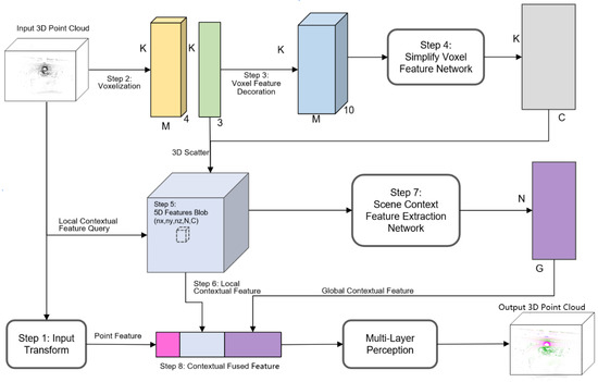
Figure 1.
Fast Context-Awareness Encoder for LiDAR Point.
The pseudo-code for the Fast Context-Awareness Encoder network is as Algorithm 1:
| Algorithm 1: Construction steps of the FCAE network | |
| Input: | Points: (N, 4); batch_size: N |
| Point cloud range: (x_min, y_min, z_min, x_max, y_max, z_max); | |
| Voxel_size: (x_size, y_size, z_size); | |
| Maximum number of points in each voxel: M; Total number of voxels after voxelization: K; | |
| Step 1: | Feature transformation of point |
| ① | coords_part = points[:, 0:3]; intensity_part = points[:, 3]; |
| ② | x = ReLU(BatchNorm1d(Conv1d(coords_part))); ▷ For three times max(x, 2, keepdim = True); ReLU(BatchNorm1d(Linear(ReLU(BatchNorm1d(Linear))))); Linear(64, 9); |
| ③ | trans_coords_part = coords_part + bias; coords_part = coords_part × trans_coords_part; ▷ T-net tsn_out = concat(coords_part, intensity_part); ▷ output the transformed point features (N, 4) as the input of Step7. |
| Step 2: | Feature Voxelization |
| ① | batch_voxels (K, M, 4) = Dense Voxels; features_ls = [batch_voxels] |
| ② | points_mean = sum(batch_voxels[:, :, :3])/K; xc, yc, zc = batch_voxels[:, :, :3] - points_mean; ▷ the distance between each internal point and the arithmetic mean of the points in the voxel. Feature matrix (K, M, 3); features_ls.append(xc, yc, zc) |
| ③ | Voxel_Coordinates (K, 3) ▷ it is used as the input of Step 4; xp, yp, zp =batch_voxels[:, :, :3]-Voxel_Coordinates*x,y,z_size + x,y,z_offset ▷ the distance between each point and the center of the voxel. Feature matrix (K, M, 3); features_ls.append(xp, yp, zp). |
| Step 3: | Feature decoration |
| ① | Features (K, M, 10) = features_ls |
| ② | paddings_indicator(K,M); ▷ reset the filling point to 0 mask == unsqueeze(mask, −1).type_as(features); ▷ (K, M, 1) features = features × mask ▷ Feature Decoration matrix(K, M, 10) is used as the input of Step 3. |
| Step 4: | Simplify VFE feature extraction |
| ① | Feature Decoration matrix(K, M, 10) ReLU(BatchNorm1d(Linear (10, C))); ▷ output (K, M, C), C refers to the output feature dimension, C = 64 in the paper; |
| ② | features = max(x, dim = 1,keepdim = True); ▷ output the feature dimension (K, 1, C); |
| ③ | voxel_features = features.squeeze(dim = 1); ▷ Remove redundant dimensions, matrix(K, C)as the input of Step 4. |
| Step 5: | Converting dense features to 5D feature blob |
| ① | nx = (x_max − x_min)/x_size; ny = (y_max − y_min)/y_size; nz == (z_max − z_min)/z_size; |
| ② | for sample_index in range(batch_size): indices == X × self._ny × self._nz + Y × self._nz + Z; ▷ Global index, where (X,Y,Z): indices of voxel grids in x,y, z-axis, calculated by Voxel_Coordinates (K, 3) canvas_3d[:, indices] == voxel_features; end for |
| ③ | canvas_3d (batch_size, C, self._nx × self._ny × self._nz); canvas_3d == canvas_3d.view(batch_size, C, nx, ny, nz) ▷ output shape (batch_size, C, nx, ny, nz), C = 64 in paper, and is used as the input of Step 5 and Step 6. |
| Step 6: | Local feature extraction |
| ① | for batch_idx in range(batch_size): batch_mask == batch_idx local_feats == canvas_3d[batch_idx, :, x_coords, y_coords, z_coords]; local_feats[batch_mask, :] == local_feats ▷ the local feature (N, C) as the input of Step7. end for |
| Step 7: | Scene global feature extraction ▷ canvas_3d(batch_size, C, nx, ny, nz) |
| ① | max_pool3d(relu(Conv3d(C, C/2))); ▷ For three times |
| ② | Linear((nx/8) × (ny/8) × (nz/8) × (C/8, G) ▷ Global feature (N, G). G is the set global feature dimension, which is 1024 in the paper. The matrix is as the input of Step 7. |
| Step 8: | Point-Voxel-Global feature fused network |
| ① | fuse_feats == concat([points, local_feats, global_feats], dim = −1) ▷ Combine that point features, the local feature and the global features, fuse_feats (N, 4 + C + G); |
| ② | MLP perception: MLP(F) = log_softmax(Relu(FC3(Relu(FC2(Relu(FC1)))))) ▷ shape = (N, D), D is the number of semantic segmentation classes. |
3.2. Points’ Invariant Feature Network
To capture local and global features across different abstraction levels, this paper proposes a method combining point cloud features from three different levels to fully integrate the semantic features of the context. These levels include (i) the invariant feature of the point, (ii) the context semantic information around each point, and (iii) the high-level abstract feature of the global scene context.
The initial point feature extraction is performed to preserve the rotation invariance, translation invariance, and scale invariance of the point cloud. In this paper, the network employs the T-net module from PointNet, a transformation function based on the data itself. The generated point cloud rotation matrix is multiplied by the input point cloud data to perform the affine transformation. The purpose of this module is to fully retain the point features of the original point cloud by training the transformation matrix. The purpose of this module is to completely retain the point features of the original point cloud by training the transformation matrix, corresponding to step1 in pseudo code.
The initial input data P∈RN×4, the algorithm, refer to the code design of PyTorch in PointNet’s 3 × 3 T-net transformation for its first three-dimensional data matrix coords_part (N, 3). It is expanded by passing through three Conv1d convolution unit. However, in the parameters of the convolution, the output channel of the last layer is set to 256, which is not as large as the gap with the channels set in PointNet. The design of the network layer is shown in Figure 2. Following the convolutions, the data goes through a max-pooling layer, two linear full connection unit, and a linear layer, reducing the dimension to 9.
where, CU(X) = Relu(BatchNorm1d(Conv1d(X))), LU(X) = Relu(BatchNorm1d(Linear(X))).
Trans(coords_part) = Linear(LU2(LU1(Max(CU3(CU2(CU1(coords_part)))))))
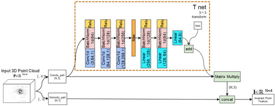
Figure 2.
T net transform for input points’ invariant feature.
After the above transformation, the output 9-dimension data can be changed into 3 × 3 feature matrix, where tij is the element of the matrix, which is then added to the bias term to get the T-net transform matrix T.
In the next step, the coords_part (N, 3) part of the original input data is transposed to represent as P′ ∈ RN×3, and T is multiplied to obtain the coordinates of the transformed point cloud:
where X″ ∈ R3×N, then the tensor X″ is transposed back to its original shape and spliced with the original Intensity_part by the Contact function to form a new tensor I ∈ RN×4 as the output matrix. The T-net transformation allows for better preservation of point features.
X″ = T · P′
3.3. Voxel Feature Network
This part is focused on the voxelization of point cloud data and the extraction of the voxel features in the network. Figure 3 shows the architecture of the network.
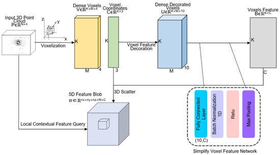
Figure 3.
Voxel feature network and local contextual feature extraction.
3.3.1. Point Cloud Voxelization
The point cloud sample data has four dimensions, denoted as P∈RN×4, where N is the total number of points in the current scene. In order to extract local context features in the feature extraction network, the point cloud is first voxelated, corresponding to step 2 in pseudo code. The purpose involves dividing the space into voxels to reduce the imbalance of points between them. By doing so, calculation power can be saved, and features can be extracted more quickly. Given the sparse points in the point cloud and uneven distribution in space, this article adopts VoxelNet’s method to transform points with an uneven density distribution into regularly distributed voxel blocks stored in memory. The first step in this process is to set the voxel grid size to be divisible by the point cloud range size; the experimental settings in this paper are (0.64, 0.64, 0.64), resulting in an integer voxel grid number K. To prevent over-calculation in the voxel grid with varying numbers of points, a proper maximum point number M is set as the sampling threshold. The output is V ∈ RK×M×4. In the next step, random sampling is applied, and point clouds below this threshold are filled with 0. This ensures that the network reduces the imbalance between different voxels.
3.3.2. Voxel Feature Decoration
After voxelating the original point clouds, the dense voxels represented by V ∈ RK×M×4 are obtained, and the corresponding voxel coordinates represented by C ∈ RK×3 are calculated to indicate the voxel indices on the x, y, and z axes in the voxel grid. In the next step of the voxel feature decoration procedure, additional relative coordinates are also calculated. These include the distance (xc, yc, zc) between each point and the arithmetic mean (centroid) of the points within the voxel, as well as the offsets (xp, yp, zp) of each point to its voxel center (physical center). The computational process for obtaining these coordinates is shown in Figure 4.
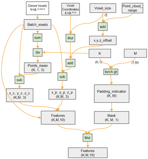
Figure 4.
Voxel feature decoration procedure.
The voxel feature decoration method described in the paper is an extension of the PointPillar algorithm. The difference is that our method enhances feature extraction along the z-axis. In the PointPillar approach, the compression on the z-axis can map the feature map into a 2D pseudo image from 3D data, and then in the backbone part, reduce the computational complexity of using Conv3d(Time ~ O(k3·nx’·ny′·nz′·Cin·Cout)) by Conv2d(Time ~ O(k2·nx′·ny′·Cin·Cout)), where k is the kernel size, nx′, ny′,nz′ are the size of the output feature map, Cin, Cout are input channel and out channel, respectively. The point features are aggregated by using the maximum pool operation in the Pillar, which can destroy the local fine-grained information and yield unsatisfactory performance, especially for the small objects and the stacked objects on the z axis.
Our method uses Con3d for convolution calculation to extract features of voxels and the complete voxel structure, rather than Con2d on the pseudo-image. This allows the offset on the z-axis from the center coordinates to be calculated, resulting in a voxel-based feature representation that expands the feature dimension of the enhanced data and captures more spatial feature information. The point cloud data is augmented to a 10-dimensional feature matrix (x, y, z, r, xc, yc, zc, xp, yp, zp) from a 9-dimensional feature matrix (x, y, r, xc, yc, zc, xp, yp, zp) of the PointPillar algorithm.
Due to the presence of xc, yc, zc, xp, yp, zp values, no distinction is made between valid points in voxels and filled zeros. Therefore, this paper retains the method of using masks in VoxelNet to reset these filled feature points to 0. Unlike the VoxelNet network, where the mask operation is executed once in each layer of stacked VFE modules in the later stage, in this work, it is directly executed after the generation of enhanced voxel data to ensure that the input data is purer. This results in the creation of enhanced densely decorated voxels, represented by U ∈ RK×M×10, which serve as the input to the Simplified Voxel Feature Network (SVFE), corresponding to step 3 in pseudo code.
3.3.3. SVFE
The point cloud features can be learned effectively by extending the data dimension to 10 dimensions. As shown in Figure 3, the voxel feature extraction (VFE) in our paper is similar to VFE in VoxelNet, but with one key difference: it only uses one layer of VFE. This is because, in the subsequent steps, the point feature and the voxel feature are concatenated to obtain the local aggregation features of each voxel, eliminating the need for multiple VFE layers. This can significantly reduce the computation of this step. The SVFE proposed in our paper is inspired by the PFN layer used in the PointPillars network. The SVFE contains only a fully connected layer and a max operation, with the fully connected layer using a (10, C) linear layer. The output dimension is a matrix of (K, M, C), where C is the output feature dimension of the voxel. The second dimension is then max-pooled to obtain an output matrix of (K, 1, C). This allows for the feature information of the voxelated point cloud to be described as interactive information that is directly extracted from the local aggregation point. Here the formula for this step is as follows: the input variable is the decorated voxel U ∈ RK×M×10, and the output tensor is B ∈ RK×C, corresponding to step 4 in pseudo code.
SVFE(U) = Max(ReLU(BatchNorm1d(Linear (U))))
3.3.4. Generate 5D Spatial Feature Blob
Non-empty voxels are processed in the SVFE, and these voxels correspond to only a smaller part of the original space. Here, it is necessary to remap the obtained non-empty voxel features back into the original 3D space, i.e., the dense voxel feature represented by B ∈ RK×C. This involves using a 3D scatter to combine the spatial information of the voxel inner points with the dense voxel feature, resulting in a 5D feature matrix π ∈ Rnx×ny×nz×N×C. The indices of the voxel grids in the x, y, and z-axis are calculated using their Cartesian topological structure; the formula is as follows:
where X, Y, and Z are their values in three dimensions, and nx, ny, and nz represent the number of grids along the x, y, and z-axis, respectively. The feature data of the voxel points are then put into the voxel grid indices to create the output 5D feature blob, where N is the number of points in the data queue and C is the dimension of voxel feature extraction. Due to the sparsity of the point cloud data, about 90% of the voxels are empty, which can greatly reduce the memory and computational consumption of backpropagation, corresponding to step 5 in pseudo code.
Ind = X × ny × nz + Y × nz + Z
3.4. Scene Context Feature Extraction Network (SCFEN)
The SCFEN network proposed in the paper aims to extract scene context features from the local contextual features of the point cloud. By combining the previously extracted local point-space features, the network can produce an initial global feature that captures the awareness of the scene context in the point cloud. This process aggregates context information from voxel local features to abstract higher-level point cloud information. Figure 5 shows the architecture of the network.
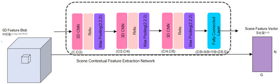
Figure 5.
Scene context feature extraction network.
The 5D local feature blobs are fed to the SCFEN network as input to obtain the global context features. The process is similar to the convolutional middle layers (CML) in VoxelNet, which use three Conv3d layers for feature extraction. The difference is that it considers max-pooling after each Con3d layer to retain more significant local features for each voxel feature. Compared with VoxelNet, the initial global features extracted by this method can highlight the fine-grained features of the point cloud to a greater extent.
The procedure for network implementation is described here. The 5D spatial feature matrix is passed through three sets of convolutional maximum pooling units (including the Conv3d layer, Relu activation layer, and max-pooling layer). The channels are halved per unit. The resulting features are then fed into a fully connected layer to obtain the initial global feature vector S ∈ RN×G.
where, CU3d(X) = Max(Relu(Conv3d(X)))
SCFEN(π) = FC(CU3d3(CU3d2(CU3d1(π))))
The default value of G is 1024. This paper also conducts experiments to compare the performance of the global feature with a dimension of 512. In this step, the output (N, G) matrix is used as the scene context feature vector of the global feature. After extracting the local features and sparse tensors of each voxel in the VFN network, SCFEN extends the receptive field to obtain rich shape information. Corresponding to step 7 in pseudo code.
3.5. Point-Voxel-Global Feature Fused Network
This paper presents point cloud features at three levels to fully integrate the semantic features of the context. Figure 6 shows the architecture of the network. In the first part, the T-Net transformation extracts invariant point features, resulting in the output I ∈ RN×4. The second part uses voxel coordinates to sample surrounding features, generating a 5D spatial feature matrix π ∈ Rnx×ny×nz×N×C. This, along with corresponding position information, forms the local context awareness information L ∈ RN×C. The third part presents a high-level abstract global feature, represented by S ∈ RN×G, which combines point position features and voxel context features from the 5D abstract voxel feature matrix. Since the global feature extraction process integrates the local context features from the previous section, and the local features abstract not only the position information of the point itself but also that of others, the abstract ability of this feature is stronger.
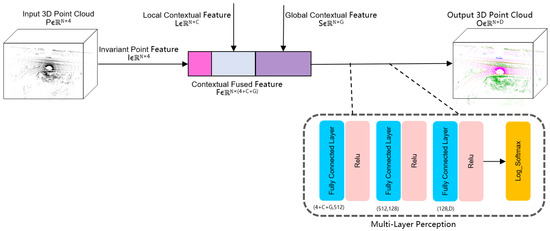
Figure 6.
Point-Voxel-Global feature fused network.
Following the extraction of context features at all levels, this paper cascades the features from all levels together to generate new abstract features. These features combine the invariant point features, the local features of voxelated points and their surrounding points, and the abstracted initial global features, each occupying different proportions in terms of their degree of importance. The specific proportion is determined by the number of channels output by each feature network.
F = Contact (I + L + S)
Here three levels of context features (I, L, and S represent the point-, local-, and global features, respectively) are fused to generate an output context feature F∈RN×(4+C+G) using the Contact function. The time complexity here is O(N·(4 + C + G)). The fused features are then extracted using a multi-layer perception (MLP) network. For the 2-dimensional data here, this network uses multiple fully connected layers to achieve higher feature expression ability than a convolutional neural network while reducing computational requirements and avoiding overfitting that may occur when using multiple convolution kernels. The time complexity of single-layer Conv is O(Cin⋅Cout⋅k2⋅Hout⋅Wout), where C represents the number of channels of input tensor, k represents convolution kernel size, and Hout and Wout represent the height and width of the output tensor, respectively. The time complexity of single-layer MLP is O(Win⋅Wout), where Win and Wout represent the input and output tensors, respectively, so the time complexity of MLP is lower than Conv’s. The following is the formula of the MLP network for the F variable, where the fully connected calculation is using Linear.
MLP(F) = log_softmax(Relu(FC3(Relu(FC2(Relu(FC1(F)))))))
The MLP consists of three sets of fully connected layers (FC1, FC2, FC3), and the number of output channels D corresponds to the number of final classifications. After obtaining the features, the output is represented as O ∈ RN×D, and then passed through the log_softmax activation function, which normalizes the exponential function. This maps the output of multiple neurons to a range of (0,1), with the normalized sum equal to 1. Finally, the entire point cloud segmentation network calculates the probability distribution for each classification to obtain the semantic information of each output point, corresponding to step 8 in pseudo code.
4. Experiment Result
Our 3D point cloud semantic segmentation network was trained on the NVIDIA Tesla T4 GPU. In this experiment, the batch size was set to 4 during network training, and the Adam gradient optimizer was used to optimize the learning rate, which was adjusted according to the number of epochs trained. The initial learning rate was 0.001 and was reduced to 0.1 times every ten epochs. The learning rate decreased gradually during the experiment to avoid a large oscillation range that impedes quick convergence.
As shown in Figure 7 of the training, the accuracy value quickly increased to approximately 0.9, while the training loss decreased rapidly. After completing model training, the prediction result was obtained from the validation set. This study experimented using voxel sizes (0.64, 0.64, 0.64) and a training time of 76,434 s.
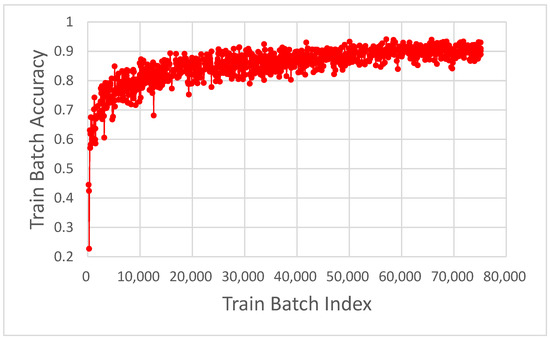
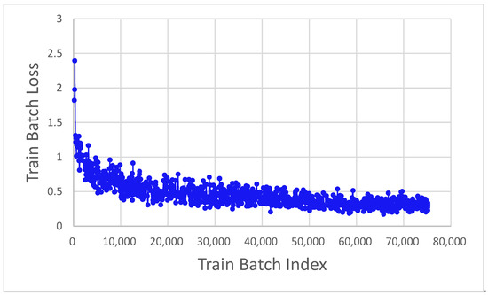
Figure 7.
The graph of accuracy and loss with training batch index.
4.1. Dataset
Semantic-KITTI [32] is one of the large-scale datasets for 3D LiDAR point-cloud segmentation, including semantic and panoptic segmentation. The dataset is about 80 G and divided into 22 sequence subdirectories. In all experiments in this paper, the data with Label in the sequences is divided into the training and test sets based on a 6:1 ratio, and the experiments will be conducted in the dataset. The dataset contains 34 classes, as follows (Table 1):

Table 1.
Combined class table for 34 classes data in semantic KITTI.
0: “unlabeled”, 1: “outlier”, 10: “car”, 11: “bicycle”, 13: “bus”, 15: “motorcycle”, 16: “on-rails”, 18: “truck”, 20: “other-vehicle”, 30: “person”, 31: “bicyclist”, 32: “motorcyclist”, 40: “road”, 44: “parking”, 48: “sidewalk”, 49: “other-ground”, 50: “building”, 51: “fence”, 52: “other-structure”, 60: “lane-marking”, 70: “vegetation”, 71: “trunk”, 72: “terrain”, 80: “pole”, 81: “traffic-sign”, 99: “other-object”, 252: “moving-car”, 253: “moving-bicyclist”, 254: “moving-person”, 255: “moving-motorcyclist”, 256: “moving-on-rails”, 257: “moving-bus”, 258: “moving-truck”, 259: “moving-other-vehicle”. To simplify the classification process, classes with similar properties were combined, and the class “unlabeled” were ignored. This resulted in the retention of 19 classes used for training and evaluation.
4.2. Evaluation
4.2.1. Qualitative Evaluation Metric
In Figure 8, several semantic segmentation results generated by the 3D point cloud segmentation network on the Semantic KITTI test set are presented for qualitative evaluation. Each color represents a different semantic class. The segmented graph shows that the ground points are divided into roads and sidewalks. Also, it accurately distinguished objects, such as the edges of road sidewalks, from roads.
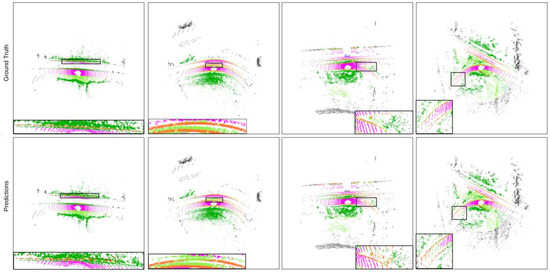
Figure 8.
The segmentation effect comparison of our algorithm and ground truth on the semantic KITTI test set.
The visible segmentation results closely matched the ground truth in the semantic KITTI dataset.
In the comparison experiment presented in the paper, Figure 9 shows the comparative segmentation effect when the voxel sizes are (0.64, 0.64, 0.64) and (0.32, 0.32, 0.32). The voxel grid size is set to be divisible by the point cloud range size, resulting in an integer voxel grid number. While the segmentation effects of some places with voxel sizes (0.32, 0.32, 0.32) may be better than those with voxel sizes (0.64, 0.64, 0.64), there are also some objects where the segmentation is worse. The difference in qualitative evaluation is not significant. For example, the side of the road in the figure with the voxel size (0.64, 0.64, 0.64) is unclear, but the effect of the road extending forward in the figure with the voxel size (0.32, 0.32, 0.32) is not as good as the original.
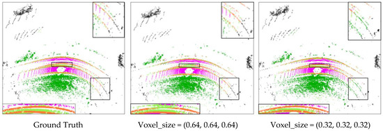
Figure 9.
The segmentation effect of our algorithm with different voxel sizes on the semantic KITTI test set.
Figure 10 illustrates how two sets of point clouds (as Group 1, Group 2 shown) are segmented by removing or adjusting corresponding components in the ablation experiment. The figure depicts that removing each of the three components from the network leads to a varying degree of accuracy loss, with the local feature module having the greatest impact and the point feature module having the lowest. Since the global module plays a crucial role in the output feature, the paper only modifies the output dimension value of the module, setting it to 512. Through comparison of experimental effects, it is observed that this modification also results in a significant loss of the segmentation effect.
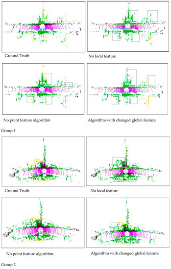
Figure 10.
The segmentation effect of the ablation experiment of two groups.
4.2.2. Quantitative Evaluation Metric
mAP
In the experiments, the accuracy of the algorithm in the prediction process is determined by the ratio of the predicted truth value to the sample dataset. So, mAP (Mean Average Precision) is considered to calculate as an evaluation metric for the model. The mAP of our method is 0.7998.
In point cloud semantic segmentation, mIOU is often used as the metric for judging the models, which can measure the accuracy of each pixel. This paper uses the MIoU value to calculate the prediction accuracy of the model.
MIoU
In order to evaluate the proposed method, we follow the official guidance to leverage mIoU as the evaluation metric. It can be formulated as follows: we follow the official guidance to leverage mIoU as the evaluation metric defined in Semantic KITTI [32].
The accuracy of our proposed model was evaluated using MIoU in 19 categories, and the quantitative results are presented in Table 2, along with a comparison to other state-of-the-art methods for point cloud segmentation. While the average IoU score of our model (68.9%) is slightly lower than that of the model with the highest score (the Point-Voxel-KD algorithm reached this value of 69.3 after the data set was enhanced by applying fine-tuning, flipping, and rotation tests), it exhibits the best performance in 7 out of the 19 categories. Our model performs better, particularly for small targets like people and objects that are easily confused in the z-axis direction, such as motorcycles, motorcyclists, and bicycles. Additionally, the average detection time of our model is 90 ms, which is relatively short compared to the inference time of state-of-the-art algorithms.
Table 2.
Quantitative results of our proposed method and other LiDAR semantic segmentation methods on proposed semantic KITTI test set in this article (Our method performs higher in several classes, and the MIoU is close to the best-performing algorithms, The bold numbers are the highest value of MIoU in each classification in experiments.
4.2.3. Comparative and Ablation Experiments
In this paper, a comparative experiment was conducted using an initial voxel size value of (0.64, 0.64, 0.64), and the experiment was repeated with voxel size set to (0.32, 0.32, 0.32). To avoid memory overflow, the batch was set to 1, and the corresponding training time was extended by almost four times. The experimental results showed that the MIoU increased by 0.6 percentage points to 69.5, and the accuracy rate increased by 1.84 percentage points to 0.8182. It was observed that the accuracy and MIoU of the model improved with a reduction in voxel size. However, the training time increased significantly, the gradient descent was slower, and the training was less likely to converge. Additionally, for some classifications, the segmentation effect was worse than that of the original model. Consequently, the experiment determined that (0.64, 0.64, 0.64), was the optimal voxel size.
The article includes ablation experiments that involve modifying the values of each component, the results are shown in Table 3. As the global feature module is the basis of feature extraction and its features cannot be eliminated, the module reduces the dimension occupied by its features, thereby reducing the proportion of the fused features. The experiments also involve eliminating the point feature module and the voxel feature module in the perception network, and the results of these ablation experiments are as follows.
Table 3.
The final performance of ablation experiments of each component (When the features of various levels are abused in the base network, the MIoU value is greatly reduced).
This paper presents the ablation experiments on the three fusion modules. The experiments revealed that removing the point feature module led to a reduction in MIoU of 4.2%. Similarly, when the voxel feature module did not participate in the fusion feature, the loss in MIoU was significant, with a reduction of 16.6%. Furthermore, reducing the dimension of the global feature output to 512 also resulted in a loss of MIoU, with a reduction of 13.3%. These results suggest that each module of the proposed feature network plays a relatively important role in improving the accuracy of point cloud segmentation.
5. Discussion
To improve our point cloud segmentation network, the following design methods can be considered for future work: To optimize point cloud segmentation, a technique involves dividing the point cloud data into sector data blocks based on its 360-degree distribution around the origin. The sector data blocks are densest near the origin and larger further away from the center radius, where the point cloud is sparser. This blocking method results in a more balanced distribution of data within the blocks, which can improve segmentation accuracy for details and learning outcomes while avoiding the omission of details. Within the segmented sector data block, the data of 360 degrees can be further divided into several equal parts in different directions, enhancing the segmentation process. In addition to the fan-shaped block, the point cloud voxels can be designed vertically by dividing the data into different-sized voxels on the z-axis. However, in actual point cloud data, most data above a certain height may be sparse or blank, resulting in wasted data blocks for learning. To optimize this, the data above a certain height can be identified as sparse data and treated separately, while the data below this height can be normally divided into equal parts. The upper part of the data in this area is longer than the other parts but relatively sparse, so balancing the distribution of the point cloud divided on the Z-axis can avoid invalid division based on height. To address the issue of characteristic data loss due to the pooling layer on the original layer data, pyramid zooming and cascading operations can be performed on the network. These operations can improve the learning effect and the accuracy of point cloud segmentation.
6. Conclusions
This study examines the technique of point cloud segmentation and proposes the Fast Context-Awareness network, which demonstrates superior performance compared to other state-of-the-art methods on the Semantic KITTI dataset. Although our algorithm is lower than the one with the highest score, it exhibits the best performance in some categories. The network leverages multi-level features such as point features, voxel features, and global features to impart semantic information to points in the point cloud quickly. The logical structure of our method allows for easy parameter adjustments based on the point cloud’s characteristics. For instance, by changing the final feature dimension of the point feature module, the proportion of point features can be increased or reduced, while the proportion of local voxel features and global features can be decreased or increased. This feature network facilitates the extraction of detailed information from point clouds and yields more accurate point cloud segmentation results on datasets like Semantic KITTI. The paper also enhances the segmentation effect of feature extraction on the Z axis, making some objects with more prominent features on the Z axis, such as motorcyclists and motorcycles, better segmented than other point cloud segmentation networks. The results suggest that the proposed network may be more effective for driving datasets with large road slopes, such as coal mine alleys, where the slope may be more than ten degrees. The network can better segment stacked point clouds belonging to the same object category at different heights on the Z-axis, potentially leading to improved point cloud segmentation performance.
Author Contributions
Conceptualization, D.W.; methodology, D.W.; software, T.D.; validation, T.D. and D.W.; formal analysis, T.D.; investigation, T.D. and D.W.; data curation, T.D.; writing—original draft preparation, T.D.; writing—review and editing, T.D.; visualization, T.D.; supervision, J.N. and D.W.; project administration, J.N.; funding acquisition, J.N.; resources, J.N.; validation, J.N. All authors have read and agreed to the published version of the manuscript.
Funding
This study was funded by National Key Research and Development Program of China (grant no. SQ2018YFC060172).
Data Availability Statement
The data of this study are available in a public repository that does not issue datasets with DOIs: The data that support the findings of this study are available in [“Semantic KITTI”] [33], http://semantic-kitti.org/dataset.html (accessed on 1 May 2022).
Acknowledgments
The authors would like to thank the teachers for helping them in topic selection and research and express gratitude to the reviewers for their valuable suggestions and comments.
Conflicts of Interest
The authors declare no conflict of interest.
Appendix A
Link: https://pan.baidu.com/s/15fUAjOTv2GMXdHMHJ7iRgw?pwd=fmua (accessed on 19 July 2023).
References
- Farsoni, S.; Rizzi, J.; Ufondu, G.N.; Bonfe, M. Planning Collision-Free Robot Motions in a Human-Robot Shared Workspace via Mixed Reality and Sensor-Fusion Skeleton Tracking. Electronics 2022, 11, 2407. [Google Scholar] [CrossRef]
- Lawin, F.J.; Danelljan, M.; Tosteberg, P.; Bhat, G.; Khan, F.S.; Felsberg, M. Deep projective 3D semantic segmentation. In International Conference on Computer Analysis of Images and Patterns; Springer: Cham, Switzerland, 2017; pp. 95–107. [Google Scholar]
- Qi, C.R.; Su, H.; Mo, K.; Guibas, L.J. PointNet: Deep Learning on Point Sets for 3D Classification and Segmentation. In Proceedings of the 30th IEEE/CVF Conference on Computer Vision and Pattern Recognition (CVPR), Honolulu, HI, USA, 21–26 July 2017; pp. 77–85. [Google Scholar]
- Qi Charles, R.; Yi, L.; Su, H.; Guibas, L.J. PointNet ++: Deep Hierarchical Feature Learning on Point Sets in a Metric Space. In Proceedings of the 31st Annual Conference on Neural Information Processing Systems (NIPS), Long Beach, CA, USA, 4–9 December 2017; p. 30. [Google Scholar]
- Zhou, Y.; Tuzel, O. VoxelNet: End-to-End Learning for Point Cloud Based 3D Object Detection. In Proceedings of the IEEE/CVF Conference on Computer Vision and Pattern Recognition (CVPR), Salt Lake City, UT, USA, 18–23 June 2018; pp. 4490–4499. [Google Scholar]
- Lang, A.H.; Vora, S.; Caesar, H.; Zhou, L.; Yang, J.; Beijbom, O. PointPillars: Fast Encoders for Object Detection from Point Clouds. 2019. Available online: https://openaccess.thecvf.com/content_CVPR_2019/papers/Lang_PointPillars_Fast_Encoders_for_Object_Detection_From_Point_Clouds_CVPR_2019_paper.pdf (accessed on 1 April 2022).
- Huang, X.; Wang, C.; Xiong, L.-Y.; Zeng, H. A weighted k-means clustering method for in- and inter-cluster distances in ensembles. Chin. J. Comput. 2019, 42, 2836–2847. [Google Scholar]
- Ma, L.J.; Wu, J.G.; Chen, L. DOTA: Delay Bounded Optimal Cloudlet Deployment and User Association in WMANs. In Proceedings of the 17th IEEE/ACM International Symposium on Cluster, Cloud and Grid Computing (CCGRID), Madrid, Spain, 14–17 May 2017; pp. 196–203. [Google Scholar]
- Yang, Y.; Li, M.; Ma, X. A Point Cloud Simplification Method Based on Modified Fuzzy C-Means Clustering Algorithm with Feature Information Reserved. Mathematical Problems in Engineering. Math. Probl. Eng. 2020, 2020, 5713137. [Google Scholar] [CrossRef]
- Zhou, K.; Hou, Q.; Wang, R.; Guo, B. Real-time KD-tree construction on graphics hardware. ACM Trans. Graph. 2008, 27, 126. [Google Scholar] [CrossRef]
- Woo, H.; Kang, E.; Wang, S.; Lee, K.H. A new segmentation method for point cloud data. Int. J. Mach. Tools Manuf. 2002, 42, 167–178. [Google Scholar] [CrossRef]
- Arias-Castro, E.; Chen, G.L.; Lerman, G. Spectral clustering based on local linear approximations. Electron. J. Stat. 2011, 5, 1537–1587. [Google Scholar] [CrossRef]
- Hu, X.B.; Chen, W.; Xu, W.Y. Adaptive Mean Shift-Based Identification of Individual Trees Using Airborne LiDAR Data. Remote Sens. 2017, 9, 148. [Google Scholar] [CrossRef]
- Wang, C.; Ji, M.; Wang, J.; Wen, W.; Li, T.; Sun, Y. An Improved DBSCAN Method for LiDAR Data Segmentation with Automatic Eps Estimation. Sensors 2019, 19, 172. [Google Scholar] [CrossRef] [PubMed]
- Li, J.; Sun, H.; Dong, Y.; Zhang, R.; Sun, X. Review of 3D point cloud processing based on deep learning. Comput. Res. Dev. 2022, 59, 1160–1179. [Google Scholar]
- Li, H.; Wang, J.; Xu, L.; Zhang, S.; Tao, Y. Efficient and accurate object detection for 3D point clouds in intelligent visual internet of things. Multimed. Tools Appl. 2021, 80, 31297–31334. [Google Scholar] [CrossRef]
- Su, H.; Maji, S.; Kalogerakis, E.; Learned-Miller, E. Multi-view Convolutional Neural Networks for 3D Shape Recognition. In Proceedings of the IEEE International Conference on Computer Vision (ICCV), Santiago, Chile, 7–13 December 2015. [Google Scholar]
- Garcia-Garcia, A.; Gomez-Donoso, F.; Garcia-Rodriguez, J.; Orts-Escolano, S.; Cazorla, M.; Azorin-Lopez, J. PointNet: A 3D convolutional neural network for real-time object class recognition. In Proceedings of the 2016 International Joint Conference on Neural Networks (IJCNN), Vancouver, BC, Canada, 24–29 July 2016; pp. 1578–1584. [Google Scholar]
- Zhao, Y.H.; Birdal, T.; Deng, H.W.; Tombari, F. 3D Point Capsule Networks. In Proceedings of the 32nd IEEE/CVF Conference on Computer Vision and Pattern Recognition (CVPR), Long Beach, CA, USA, 15–20 June 2019; pp. 8887–8896. [Google Scholar]
- Shi, S.S.; Wang, X.G.; Li, H.S. PointRCNN: 3D Object Proposal Generation and Detection from Point Cloud. In Proceedings of the 32nd IEEE/CVF Conference on Computer Vision and Pattern Recognition (CVPR), Long Beach, CA, USA, 15–20 June 2019; pp. 770–779. [Google Scholar]
- Ali, W.; Abdelkarim, S.; Zidan, M.; Zahran, M.; El Sallab, A. YOLO 3D: End-to-end real-time 3D oriented object bounding box detection from Lidar Point cloud. In Proceedings of the European Conference on Computer Vision, Munich, Germany, 8–14 September 2018; pp. 10–30. [Google Scholar]
- Wang, B.; An, J.; Cao, J. Voxel-FPN: Multi-scale voxel feature aggregation in 3D object detection from point clouds. arXiv 2019, arXiv:1907.05286. [Google Scholar]
- Yan, Y.; Mao, Y.; Li, B. SECOND: Sparsely Embedded Convolutional Detection. Sensors 2018, 18, 3337. [Google Scholar] [CrossRef] [PubMed]
- Chen, Y.; Liu, S.; Shen, X.; Jia, J. Fast point r-cnn. In Proceedings of the IEEE International Conference on Computer Vision, Seoul, Republic of Korea, 27 October–2 November 2019; pp. 9775–9784. [Google Scholar]
- Shi, S.; Guo, C.; Jiang, L.; Wang, Z.; Shi, J.; Wang, X.; Li, H. Pv-rcnn: Point-voxel feature set abstraction for 3d object detection. In Proceedings of the IEEE/CVF Conference on Computer Vision and Pattern Recognition, Seattle, WA, USA, 13–19 June 2020; pp. 10529–10538. [Google Scholar]
- Wang, L.; Huang, Y.; Hou, Y.; Zhang, S.; Shan, J. Graph attention convolution for point cloud semantic segmentation. In Proceedings of the IEEE Conference on Computer Vision and Pattern Recognition, Long Beach, CA, USA, 15–20 June 2019; pp. 10296–10305. [Google Scholar]
- Shi, W.; Rajkumar, R. Point-gnn: Graph neural network for 3d object detection in a point cloud. In Proceedings of the IEEE/CVF Conference on Computer Vision and Pattern Recognition, Seattle, WA, USA, 13–19 June 2020; pp. 1711–1719. [Google Scholar]
- Zarzar, J.; Giancola, S.; Ghanem, B. PointRGCN: Graph convolution networks for 3D vehicles detection refinement. arXiv 2019, arXiv:1911.12236. [Google Scholar]
- Cheng, R.; Razani, R.; Taghavi, E.; Li, E.X.; Liu, B.B. (AF)2-S3Net: Attentive Feature Fusion with Adaptive Feature Selection for Sparse Semantic Segmentation Network. In Proceedings of the IEEE/CVF Conference on Computer Vision and Pattern Recognition (CVPR), Nashville, TN, USA, 20–25 June 2021; pp. 12547–12556. [Google Scholar]
- Xie, X.; Bai, L.; Huang, X. Real-Time LiDAR Point Cloud Semantic Segmentation for Autonomous Driving. Electronics 2021, 11, 11. [Google Scholar] [CrossRef]
- Zhou, Z.; Zhang, Y.; Foroosh, H. Panoptic-polarnet: Proposal-free lidar point cloud panoptic segmentation. In Proceedings of the IEEE/CVF Conference on Computer Vision and Pattern Recognition (CVPR), Nashville, TN, USA, 20–25 June 2021; pp. 13189–13198. [Google Scholar]
- Behley, J.; Garbade, M.; Milioto, A.; Quenzel, J.; Behnke, S.; Stachniss, C.; Gall, J. Semantic KITTI: A Dataset for Semantic Scene Understanding of LiDAR Sequences. Computer Vision and Pattern Recognition, 2019. Available online: https://arxiv.org/pdf/1904.01416.pdf (accessed on 1 April 2022).
- Semantic KITTI. 2021. Available online: http://semantic-kitti.org/dataset.html (accessed on 1 May 2022).


Disclaimer/Publisher’s Note: The statements, opinions and data contained in all publications are solely those of the individual author(s) and contributor(s) and not of MDPI and/or the editor(s). MDPI and/or the editor(s) disclaim responsibility for any injury to people or property resulting from any ideas, methods, instructions or products referred to in the content. |
© 2023 by the authors. Licensee MDPI, Basel, Switzerland. This article is an open access article distributed under the terms and conditions of the Creative Commons Attribution (CC BY) license (https://creativecommons.org/licenses/by/4.0/).