MoBiSea: A Binary Search Algorithm for Product Clustering in Industry 4.0

Abstract

Proprietary systems used to modernize Industry 4.0 usually involve high financial costs. Consequently, using low-cost devices with the same functionalities, capable of replacing these proprietary systems but at a lower cost, has become an incipient trend. However, these low-cost devices usually come with electromagnetic interference problems as they are encapsulated in electrical panels, sitting alongside electromechanical devices. In this article, we present Mode Binary Search, an algorithm specifically designed for use in a low-cost automated-industrial-productivity-data-collection system. Specifically, productivity data are obtained from the availability and sealing signals of the thermoplastic sealing machines in production lines belonging to the agri-food industry. Mode Binary Search was designed to cluster sealing signals, thus enabling us to identify which products have been made. Furthermore, the algorithm determines when the manufacturing of each product starts and ends, in other words, the exact moment a product change occurs and all this without the need for operator supervision or intervention. Finally, we compared our algorithm, based on binary search, with three clustering mechanisms: k-means, k-rms and x-means. Out of all the cases we analyzed, the maximum error committed by Mode Binary Search is limited to 2.69%, thereby outperforming all others.

1. Introduction

The concept of Industry 4.0 aims to integrate machinery, devices and sensors, in other words, the physical manufacturing process, with digital parts and advanced software [1]. All this is driven by modern connected industry technologies used to predict, control, maintain and integrate manufacturing processes. As a result, their impact is expected to be far-reaching in future manufacturing systems and, therefore, organizations will need to increase their investments in digital technologies [2].

Although there is a wide range of devices and equipment capable of modernizing the industry, the proprietary systems used tend to involve a high financial investment. In most cases, they are encapsulated systems, implementing them is expensive and their communication protocols differ. Consequently, several proposals have analyzed the possibility of adopting low-cost devices in industrial environments. Although they have not yet been installed in real settings on a large scale, their usage is growing despite the difficulties encountered, such as strong Electromagnetic Interferences (EMIs), which are prone to cause both sensing and communications errors.

As a contribution towards increased industry automation through the adoption of low-cost systems and to demonstrate that systems requiring less financial investment may, nevertheless, be capable of performing the same operations as other proprietary systems, we have developed a solution that measures and monitors the variables involved in calculating the Overall Equipment Effectiveness (OEE) factor [3]. The aim is to obtain precise production parameters (availability, performance and quality) in real time in industrial settings.

OEE is a measurement tool based on the Total Productive Maintenance (TPM) concept. Its purpose is to detect and eliminate failures caused by equipment, thereby improving production, reducing costs and inventory, and increasing labor productivity. Measuring OEE enables us to identify reasons and quantify their effect in terms of poor performance, thus providing us with improvement rates and an analysis of the source of the defects. Figure 1 shows the components taken into account for the calculation of OEE: (i) the availability metric evaluates time ratio when the machine is genuinely ready to operate, (ii) the performance metric quantifies the share of time the machine can work, disregarding time losses stemming from reduced speed and, lastly, (iii) the quality metric calculates the fraction of time the machine operates at full productivity, accounting for time losses caused by defects.

Figure 1. Overall-equipment-effectiveness components.

The automatic collection of productivity data is a crucial component for maximizing efficiency, predicting and preventing problems and advancing towards greater automation in the era of Industry 4.0. It offers tangible advantages, such as real-time monitoring of machinery performance, enabling companies to promptly identify any system anomalies or failures. This, in turn, contributes to minimizing downtime and optimizing operational efficiency. Additionally, the collected data serve as a foundation for conducting predictive analysis, enabling the prediction of future trends or issues before they arise. As a result, proactive decision-making based on data is facilitated. Furthermore, these data play a vital role in the implementation of cyber–physical systems and the Internet of Things (IoT), as they provide the necessary information for automating and controlling production processes in real time.

It is important to emphasize that our work is immersed in the context of Industry 4.0 and the IoT. Within the framework of Industry 4.0, which seeks to integrate machinery, devices and sensors to achieve an effective digitalization of production processes, our algorithm makes a significant contribution. It provides a low-cost solution for measuring and monitoring the variables involved in the calculation of the OEE factor, a key element to achieve greater industrial automation. In addition, thanks to the automatic collection of productivity data in real time, our algorithm facilitates the implementation of cyber–physical systems and IoT, two fundamental pillars of Industry 4.0. On the other hand, our algorithm is used for the automation of electromagnetic-interference-filtering mechanisms, a recurring and significant problem in industrial environments, especially when using low-cost devices. We designed our algorithm to effectively eliminate erroneous signals caused by these interferences, thus improving the precision and efficiency of the system. This aspect is crucial as effective management of electromagnetic interference is vital to ensure the integrity of the collected data and, ultimately, the effectiveness of the production systems based on Industry 4.0 and IoT.

Our previous research focused on measuring availability and performance by measuring sealing signals in thermoplastic sealing machines in the agri-food industry [4]. Figure 2 presents a scheme of our low-cost system previously designed to determine the mentioned OEE, in particular the availability and performance factors. In this scheme, five parts can be observed: the industrial sealer, which performs the sealing of the containers; the relays that receive the electrical signals from the availability and sealing; the Raspberry Pi, a low-cost microcomputer programmed to receive the signals and to manage the database where EMI filtering mechanisms are applied; the database, where the signals from each line are stored; and finally, the OEE dashboard, responsible for monitoring the process.

Figure 2. Scheme of the low-cost OEE estimation system [4].

During the design and development process of our low-cost system, based on the Raspberry Pi platform, we encountered significant EMI problems in the signals we gathered; this is because low-cost devices are placed alongside other electromechanical elements. We solved this problem by eliminating the wrong signals due to EMI using two filtering mechanisms that were designed to detect and eliminate all wrong signals due to EMI [5], thereby avoiding any additional equipment. Specifically, these mechanisms make it possible to eliminate noise in two types of signals from thermosealing machines: sealing signals and availability signals. The Database Filter (DBF) is responsible for filtering the sealing signals, while the Smart Coded Filter (SCF) is responsible for filtering the availability signals of the machine.

The proposal presented in this article focuses on the DBF filtering mechanism, which enables us to determine valid sealing signals for a correct OEE calculation. This mechanism first filters signals lasting less than one second and then discards wrong signals that do not fit into a logical order of sealing signal values (in other words, a 1 and a 0). After these two operations, the system needs to know the start and end time instants for each product. Operators previously had to enter these values manually, which is cumbersome and error-prone. That is why we aim to design an algorithm capable of automatically estimating the manufactured products, as well as the sealing times for each product, without any operator supervision. We have called this algorithm MoBiSea (Mode Binary Search).

MoBiSea clusters sealing times to automatically identify products and also how many product types are involved in the industrial process. In addition, it determines the moment when the process starts and ends for each of the products. In our proposal, we validate MoBiSea by clustering the sealing-time values of various products in an agri-food industry and, more specifically, those involved in the sealing lines of a cheese factory. The products the algorithm must select and cluster are those involved in the manufacturing process; in other words, all the products in the manufacturing process in a shift, at different times and in each shift without distinction. MoBiSea provides the automation needed for our low-cost system based on Raspberry Pi. It mainly measures OEE, although it can be applied to other systems.

We compared MoBiSea against the k-means, k-rms and x-means algorithms to evaluate its performance and validate the proposal. Specifically, we analyzed the number of signals categorized in every cluster, the start and end of each cluster and detected the products made in each shift. We also compared real clusters (i.e., the products that have been manufactured) with those our algorithm detected, as well as the clusters estimated via the x-means algorithm, which is a version of k-means that enables us to determine the optimal number of clusters. The results, which we present in Section 4, show that the number of clusters estimated via x-means is not correct in most of the cases we analyzed. Furthermore, we show that k-means, k-rms and x-means cannot correctly estimate the number of signals in each of the clusters, nor the start and end instants in the manufacturing of each product. On the other hand, MoBiSea can achieve such goals with a maximum error of 2.96%, which we can consider negligible for the purpose of OEE calculation.

The remainder of this article is structured as follows: in Section 2, we describe the k-means, x-means and k-rms algorithms and the binary search and we discuss some studies related to our proposal. The MoBiSea algorithm is presented in Section 3, in which we clearly detail all its relevant and unique aspects. We also comment on the results after validating our proposal. MoBiSea is compared with k-means, k-rms and x-means in Section 4. Finally, Section 5 presents the most important conclusions and refers to future work.

2. Related Studies

There is currently a range of algorithms aimed at clustering data. Clustering consists in putting data into several groups, so that the data in one cluster have a maximum level of similarity; conversely, the data between clusters should have a minimum similarity [6]. k-means and x-means are two of the most widely used clustering algorithms in unsupervised learning. k-means groups objects into k clusters (users establish the value of k in advance), thus minimizing the sum of distances between each object and its cluster centroid, while x-means is a variation of k-means in which the number of clusters to be obtained does not necessarily have to be defined initially, since the mechanism automatically establishes the number of clusters based on the analyzed data.

There are also algorithms that make it possible to exactly locate an element in a sorted array of data, such as binary search. This method works by repeatedly halving the array that could contain the searched data until possible locations are reduced to only one.

Some research that uses or analyzes these clustering methods (i.e., k-means and x-means algorithms), as well as studies using binary search to locate elements in a dataset, are outlined below in more detail.

2.1. k-Means and x-Means

k-means [7] is an unsupervised learning algorithm that solves the clustering problem. We consider ($X_1,X_2,$…$,X_n$) as the set of n points that we want to group into k clusters, which we will call $S_j$. The k-means algorithm finds a partition that minimizes the mean square error between the centroid of each cluster (${\mu }_j$) and all the points in it ($X_nϵS_j$). The clustering function is given by the following equation [8]:

$$J=\sum _{j=1}^k\sum _{nϵS_j}^{}{∥X_n-{\mu }_j∥}^2$$

(1)

where ${\mu }_j$ is the arithmetic mean of the data in set $S_j$ and is defined as:

$${\mu }_j=\frac{1}{N_j}\sum _{nϵS_j}{X}_n$$

(2)

k-means is easy to implement and it has good scalability in terms of data. The clear disadvantage of this clustering method is that we first have to manually state the number of clusters we want to divide the dataset into.

The x-means mechanism [9] overcomes this drawback, since it does not require users to define the number of clusters; instead, it preprocesses the data so that it can estimate the appropriate number of clusters depending on the data to be grouped. Although it is based on k-means, it enables us to automatically check several clusters within a variable range.

Specifically, the x-means algorithm starts with a number of clusters (k) equal to the lower limit of the given range ($k_{min}$) and adds clusters to it until it reaches the upper limit ($k_{max}$). During this process, it calculates the Bayesian Information Criterion (BIC) for each of these solutions and finally selects the one with the best score.

In some studies, k-means is applied in a variety of areas, is compared with other mechanisms and is even improved. Rahamathunnisa et al. [10] propose a system based on k-means and multi-support vector machine (multi-SVM) to detect diseases in vegetable and organic products. Image processing that considers color, shape, size and texture is used for that purpose. The k-means algorithm is then applied to these characteristics to cluster the infected elements. The authors compare the k-means clustering and SVM algorithm with digital image processing in MATLAB, resulting in a proposal that is more precise and takes less time. We do not perform image processing to identify products, but instead determine the number of clusters based on variations in statistical modes in sealing-time values.

Using the Sobel operator and k-means, Siswantoro et al. [11] automatically segment food product images to identify them. The Sobel operator enables them to determine the region of interest and they then use the k-means clustering mechanism to separate the object from its background, thereby clearly identifying the product in question. The authors state that the identification results are more precise with the combination of Sobel and k-means than with k-means alone. Although the objective in our proposal is also to identify products passing along a production line, we do not use an image-recognition system; instead, we use sealing times to identify the products made at any given time.

Hüseynli et al. [12] use the k-means algorithm to categorize electronic commerce products by using text mining to automate technical specification extraction. They do this by first preprocessing the dataset and extracting attributes from a set. The processed data are product price, availability, product image and specifications. They are then clustered using k-means. The results show an effectiveness of 98%. The data do not have to be preprocessed in our proposal, however, and the results are 100% effective.

Considering production requirements in terms of product variety and related planning tasks, Hochdörffer et al. [13] propose a clustering method called Product Variety Management (PVM) capable of handling binary data related to the production process (in other words, data describing whether production technology applies to a product variant) and metric data related to production capacity (data describing capacity to apply production technology in a process step). By applying this method, they manage to divide the products into clusters in which product variants have similar requirements. The results show that planning complexity in designing production networks can be reduced with PVM. Furthermore, the authors point out that traditional clustering methods (such as k-means) are not capable of handling data with mixed characteristics. Our proposal works with data with the same characteristics; an algorithm applying mixed characteristics to determine the products made, and the moment their production starts or ends, is not required.

Noorbehbahani and Mansoori [14] address the limitations of traditional approaches to network-traffic classification. Specifically, they propose semi-supervised classification methods, since modern traffic classification methods, based on machine learning, require a large amount of labeled data to extract a precise classification model, considered costly and time-consuming. Their new semi-supervised method is based on x-means, along with a new label-propagation technique. The precision of the proposed method demonstrates its effectiveness in learning to classify network traffic using limited labeled data.

In order to address accuracy issues and reduce the number of iterations required by the k-means algorithm, Avishek and Dipankar [15] propose a modified version called the k-rms clustering algorithm. This modified algorithm incorporates changes that enhance both its accuracy and efficiency compared to the original k-means algorithm. The authors conducted experiments using 12 datasets obtained from the web archive of the University of California to evaluate the performance of the k-rms algorithm. The results obtained demonstrate significant promise and show improved outcomes compared to the traditional k-means algorithm, as shown in the comparison we have carried out.

Imamura et al. [16] propose a technique for automatically extracting moving objects in videos using the x-means clustering method. Their proposal enables the feature points in each video frame to be extracted based on affine motion parameters. Experimental results reveal that the approach accurately extracts the various objects. However, in our case, x-means returns wrong values in terms of the number of clusters for the shifts we studied, as we show in Section 4.

2.2. Binary Search

As we will see in Section 3, our MoBiSea mechanism uses a method similar to binary search as it splits the data in half at each iteration, so that it can detect when a product change occurs during manufacturing. The binary-search algorithm, also known as half-interval search or logarithmic search, is an efficient iterative search algorithm that works with a sorted array and chops the search space into two halves in every iteration. Specifically, it compares the required value with the middle element in the sequence; if the element is not found in that position, the half where the element has not been found is eliminated and the required value is searched for in the other half by marking its middle element. If the element is not found, the process is repeated until the match is found or the array is exhausted (see Figure 3). The binary-search functions are detailed in Algorithm 1.

Algorithm 1: Binary Search

$R_1{R}_2$…$R_N$ log table whose keys are in ascending order $K_1<K_2<$…$<K_N$; the algorithm searches for a given argument K l is the bottom pointer of the chosen dataset u is the top pointer of the chosen dataset i is the midpoint of the chosen dataset Step 1 [Start] The following is established $l\leftarrow 1,u\leftarrow N$ Step 2 [Obtain midpoint] At this point we know that if K is in the table, it fulfills $K_l\le K\le K_u$. If $u<l$ the algorithm ends unsuccessfully. Otherwise, $i\leftarrow \left[\right(l+u)/2]$ will be established, approximating the midpoint in the table Step 3 [Compare] If $K<K_i$, go to Step 4; if $K>K_i$, go to Step 5; and if $K=K_i$, the algorithm ends satisfactorily Step 4 [Adjust u] Establish $u\leftarrow i-1$ and go back to Step 2 Step 5 [Adjust l] Establish $l\leftarrow i+1$ and go back to Step 2

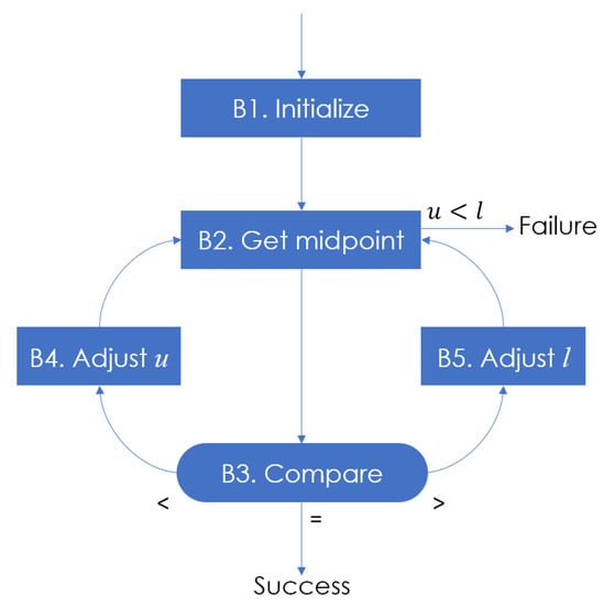
Figure 3. Binary Search [17].

The advantage of this algorithm is that it can be applied to both linear-array data and binary-search trees; it is also the most efficient method for finding items in a sorted array. However, as the algorithm only works with sorted arrays, it usually requires data preprocessing. Binary search is one of the most widely used search mechanisms applied to a dataset. Several authors have written papers based on binary search, some of which are shown below.

Since binary-search comparisons require n elements to be split in half in each iteration and matching to the key, Vuyyuru et al. [18] propose reducing the expected number of comparisons during the search process. They present a new algorithm that decreases the average number of comparisons required to search for an element depending on its size, thereby showing there are fewer search steps when only elements the same size as the key are considered. This research needs to know the element size to reduce the average time needed to lessen the comparison size, as well as the searched key. In our proposal, we are searching for a switch value for data produced continuously in the production shift, without knowing the size and the value we are looking for in advance.

Jacob et al. [19] combine binary search with linear search to create a new algorithm that offers an efficient way of searching for a specific key item in an unsorted matrix, achieving that goal within a limited time. The authors address the problems of each algorithm separately, since every element is queried and compared with the key element sequentially in the linear search; for the binary search, the data must be sorted in some way, so it is time-consuming. In our case, unlike this proposal, the data do not have to be sorted, since the signals are processed in the same order in which they are generated during production.

Bai et al. [20] also published a study on binary search. They propose an improved binary-search algorithm based on combining dynamic binary search and the backward binary-search algorithm. Experimental results show that the improved algorithm significantly decreases search times and the quantity of transmitted data compared to the traditional binary search, thus improving efficiency. More specifically, the results show the search has decreased by 75% and traffic by 85%.

MoBiSea enables us to determine the exact point when the product change occurs in the production process, calculates clusters efficiently and does not require data sorting, since the data are processed in the order in which they occur. We also compared MoBiSea with k-means, x-means and k-rms clustering mechanisms in terms of cluster detection, precision in detecting the start and end of the manufacturing of each product and the number of units forming each cluster, and we obtained highly positive results.

3. MoBiSea: Mode Binary Search

MoBiSea was developed to address the need to automate the DBF, our EMI filtering mechanism designed for OEE monitoring using low-cost devices. With the DBF mechanism, we can filter valid sealing signals, thereby avoiding wrong signals due to EMI; however, part of the process was performed manually, since operators had to manually enter into the system the time instants when a product changed during manufacturing. MoBiSea was created to avoid this scenario so that (i) manufacturing shift data, (ii) the start and end of each product and (iii) the units of each group of products involved in a shift are all entered into the system automatically.

Algorithm 2 shows the operation of MoBiSea. First, two key parameters are initialized and defined. They are: (i) the number of signals each interval contains ($isize$) and (ii) the $threshold$ applied to the mode values in every signal group. The data structure ($intervalMode$) used afterward is also declared. This data structure will comprise the $start$, $end$ and $mode$ of each interval.

The algorithm obtains signals from the database, stores it in the $signals$ array and calculates the modes of each interval by assigning it to the $ims$ array. Mode changes are obtained after this operation and are stored in the array $mcs$. The $getModeChanges$ function is used for that purpose. This function is responsible for detecting when the difference between the mode of one interval compared with another is more than the established difference ($threshold$). Next, the exact signal in which each product change occurs is sought in the array with mode changes.

The end condition of the $getSignalProductChange$ recursive function is that the number of signals taken in each interval ($isize$) is less than or equal to one; in other words, it is a single signal. This is the signal in which the mode change occurs and, therefore, the signal in which the product change occurs. For that purpose, MoBiSea takes both the interval in which the change occurred and the previous one, splits the clusters into half the signals as in the previous interval and determines the change in the exact signal in which it occurred.

MoBiSea is similar to binary search because it divides the previously taken dataset into two to find the exact product change signal. Specifically, MoBiSea has two clearly differentiated parts: The first, which we refer to as the ‘initial stage’, is responsible for determining the number of different products that have been manufactured during the analyzed shift and another one to determine the exact time when a product change takes place.    

Algorithm 2: Mode Binary Search (MoBiSea)

Figure 4 provides a graph of how MoBiSea operates. It shows the two parts into which the process is divided: the first, consisting of determining the number of products, is represented in the top part of the figure, since the signals are grouped into $isize$ clusters and their statistical mode is calculated. Consequently, when it is observed that ($\mid m_{\alpha }-m_{\alpha +1}\mid >threshold$), for example, the algorithm detects a product change during the manufacturing process (which appears as a color change in the top rectangles in the figure).

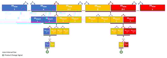
Figure 4. MoBiSea operation.

As a result of this first step, the system determines the number of clusters, in other words, the number of different products that have been made during the shift analyzed.

The bottom rows of the figure show the second part of the algorithm, since once the product changes are detected, MoBiSea performs a recursive process to precisely determine the final sealing signal of a product and, therefore, the beginning of the next. Specifically, MoBiSea reduces the number of signals to be analyzed ($isize$) and recalculates the modes of each new interval to finally detect the last sealing signal of a product and the change to a different product.

In summary, the algorithm has these distinct phases:

• Signal Collection: The algorithm collects a set of signals from the database, creating a sequence of signal values: s[1], s[2], …, s[n].
• Mode Calculation: Next, the algorithm divides this signal sequence into intervals of size $isize$ and calculates the mode of each interval. This produces a new sequence of modes m[1], m[2], …, m[n/isize].
• Mode Change Detection: The algorithm then identifies the indices i in this mode sequence, where |m[i] − m[i + 1]| > $threshold$. These indices are stored in the array $mcs$.
• Binary Search for Product Changes: Finally, the algorithm searches for the exact product change by repeatedly halving the search interval, using a binary-search approach. This is equivalent to searching for the minimum index i in the $mcs$ array such that |m[i] − m[i + 1]| > $threshold$, but restricting the search to ever smaller intervals.

Validation of MoBiSea

In this section, we present the validation of MoBiSea in a real industrial setting, specifically in the agri-food industry of cheese packaging. It has a plastic thermosealing line for whole cheeses, cheese quarters and cheese wedges. We conducted a study over six days with manufacturing shifts from 06:00 to 22:00 to correctly validate the operation of the system.

Table 1 shows the real results (which we know as we monitored the entire process) and the values MoBiSea estimated in terms of different products made, for the six analyzed shifts. Concerning MoBiSea, we show the clusters we detected when we varied both the interval size ($isize$ = 25, 50, 100, 300 and 500) and sensitivity in the difference between modes ($threshold$ = 0.10, 0.05 and 0.01). Wrong values are shown in red. As can be observed, MoBiSea is capable of obtaining the number of clusters (in other words, of the different product types made) in most of the shifts and for the various configurations. However, in shift 6, MoBiSea is only correct for the following values: $isize=50$ and $threshold=0.01$. The reason is that three different products are manufactured in this shift, but only 30 units of one of these products are made, which causes MoBiSea to work well only in one configuration.

Table 1. Clusters determined by MoBiSea when varying the interval size (25, 50, 100, 300 and 500) and the threshold (0.10, 0.05 and 0.01). Wrong values are shown in red.

Shift	Real Clusters	Interval Size 25 Threshold:			Interval Size 50 Threshold:			Interval Size 100 Threshold:			Interval Size 300 Threshold:			Interval Size 500 Threshold:
		0.10	0.05	0.01	0.10	0.05	0.01	0.10	0.05	0.01	0.10	0.05	0.01	0.10	0.05	0.01
1	1	1	1	3	1	1	1	1	1	1	1	1	1	1	1	1
2	4	4	4	9	4	4	8	4	4	6	4	4	6	3	3	4
3	3	3	3	8	3	3	5	3	3	5	3	3	4	3	3	3
4	2	2	2	2	2	2	2	2	2	2	2	2	2	2	2	2
5	3	3	3	6	3	3	5	3	3	3	3	3	3	2	2	2
6	3	2	2	4	2	2	3	2	2	2	2	2	2	2	2	2

In addition, when the $threshold$ value is very small (i.e., 0.01), the algorithm does not correctly detect mode changes in the analyzed intervals, which causes it to estimate the different products manufactured incorrectly.

As a result of all the above, we consider that the $isize$ value should be set to 50, since this ensures correct operation in all regular scenarios. Furthermore, the $threshold$ should be 0.05 since that is the lowest possible value that ensures we can identify the correct number of clusters.

After checking the most-recommendable values for the $isize$ and $threshold$ parameters, we examine how the size of the intervals MoBiSea considers affects execution time. Specifically, Table 2 shows the execution times of our proposal when we vary the size variable. As can be observed, the interval size does not have a huge impact on execution time, since it is very similar for all the sizes analyzed.

Table 2. MoBiSea execution times when varying interval size.

	Interval Size
Time (s)	25	50	100	300	500
Real	0.357	0.344	0.353	0.337	0.351
User	0.635	0.603	0.618	0.581	0.606
Sys	0.072	0.070	0.072	0.069	0.073
User + System	0.707	0.673	0.690	0.650	0.679

Therefore, by way of summary, the execution time results consolidate the idea that using $isize=50$ is the best option, since it ensures precise data without compromising the execution time needed to obtain this solution.

Considering the above, Table 3 shows some of the signals our system collected in shift 5 as an example of how MoBiSea operates. Specifically, it shows signals from 701–850. The first three columns show the values of Signal ID, Timestamp and Sealing Time, respectively, for signals 701–750 and the other columns show the same information for signals 751–800 and 801–850. If we assume the aforementioned interval size of 50, MoBiSea will calculate the mode for each of these intervals (or clusters of signals) so that it can compare them and then establish whether the difference is more than the defined $threshold$. This is how MoBiSea determines whether a mode change has occurred and when, in other words, when there is a product change.

Table 3. Excerpt of signal identification, timestamp and sealing times in shift 5.

Signals 701 to 750			Signal 751 to 800			Signal 801 to 850
Signal ID	Timestamp	Sealing Time (s)	Signal ID	Timestamp	Sealing Time (s)	Signal ID	Timestamp	Sealing Time (s)
701	14:32:43.6	8.38	751	14:46:07.0	8.38	801	15:31:20.2	7.34
702	14:32:55.1	8.38	752	14:46:18.5	8.38	802	15:31:31.0	7.39
703	14:33:06.6	8.38	753	14:46:30.0	8.38	803	15:31:41.8	7.39
704	14:33:18.1	8.38	754	14:46:41.5	8.38	804	15:31:52.6	7.34
705	14:33:29.6	8.38	755	14:46:53.0	8.38	805	15:32:03.4	7.39
706	14:33:41.1	8.38	756	14:47:04.5	8.38	806	15:32:14.2	7.34
707	14:33:52.6	8.38	757	14:47:16.0	8.38	807	15:32:25.0	7.39
708	14:34:04.1	8.38	758	14:47:27.4	8.3	808	15:32:35.8	7.34
709	14:34:15.6	8.38	759	14:47:38.9	8.3	809	15:32:46.6	7.39
710	14:34:27.1	8.38	760	14:47:50.3	8.38	810	15:32:57.4	7.34
711	14:34:38.6	8.38	761	14:48:01.8	8.38	811	15:33:08.2	7.39
712	14:34:50.1	8.38	762	14:48:13.3	8.38	812	15:33:19.0	7.34
713	14:35:01.6	8.38	763	14:49:42.9	8.38	813	15:33:29.8	7.39
714	14:35:13.1	8.38	764	14:49:54.4	8.38	814	15:33:40.6	7.39
715	14:35:24.6	8.38	765	14:50:05.9	8.38	815	15:33:51.4	7.34
716	14:35:36.1	8.38	766	14:50:17.4	8.38	816	15:34:02.2	7.39
717	14:35:47.6	8.38	767	14:50:28.9	8.38	817	15:34:13.0	7.34
718	14:35:59.1	8.38	768	14:50:40.4	8.38	818	15:34:23.8	7.39
719	14:36:10.5	8.3	769	14:50:51.9	8.38	819	15:34:34.6	7.34
720	14:36:22.0	8.38	770	14:51:03.4	8.38	820	15:34:45.4	7.39
721	14:36:33.5	8.38	771	14:51:14.9	8.38	821	15:35:10.1	7.34
722	14:36:45.0	8.38	772	14:51:26.4	8.38	822	15:35:20.9	7.34
723	14:36:56.5	8.38	773	14:51:37.9	8.3	823	15:35:31.7	7.34
724	14:37:31.9	8.38	774	14:51:49.3	8.38	824	15:35:42.5	7.39
725	14:37:43.4	8.38	775	14:52:00.8	8.38	825	15:35:53.3	7.34
726	14:37:54.9	8.38	776	14:52:12.3	8.38	826	15:36:04.1	7.39
727	14:38:06.4	8.38	777	14:52:23.8	8.38	827	15:36:14.9	7.34
728	14:38:17.9	8.38	778	14:52:35.3	8.38	828	15:36:25.7	7.34
729	14:38:29.4	8.38	779	15:27:22.6	7.34	829	15:36:36.5	7.39
730	14:38:40.9	8.38	780	15:27:33.4	7.34	830	15:36:47.3	7.34
731	14:38:52.4	8.38	781	15:27:44.2	7.39	831	15:36:58.1	7.34
732	14:39:03.9	8.38	782	15:27:55.0	7.34	832	15:37:08.9	7.39
733	14:39:15.4	8.38	783	15:28:05.8	7.39	833	15:37:19.7	7.34
734	14:39:26.9	8.38	784	15:28:16.6	7.34	834	15:37:30.5	7.39
735	14:39:38.4	8.38	785	15:28:27.4	7.39	835	15:37:41.3	7.34
736	14:39:49.9	8.1	786	15:28:38.2	7.34	836	15:37:52.1	7.34
737	14:40:01.4	8.1	787	15:28:49.0	7.39	837	15:38:02.9	7.39
738	14:40:12.8	8.0	788	15:28:59.8	7.34	838	15:38:13.7	7.34
739	14:40:24.3	8.38	789	15:29:10.6	7.39	839	15:38:24.5	7.34
740	14:40:35.7	8.3	790	15:29:21.4	7.39	840	15:38:35.3	7.39
741	14:40:47.2	8.38	791	15:29:32.2	7.34	841	15:38:46.1	7.34
742	14:44:23.5	8.38	792	15:29:43.0	7.39	842	15:38:56.9	7.39
743	14:44:35.0	8.38	793	15:29:53.8	7.34	843	15:39:07.7	7.34
744	14:44:46.5	8.38	794	15:30:04.6	7.39	844	15:39:18.5	7.39
745	14:44:58.0	8.38	795	15:30:15.4	7.34	845	15:39:29.3	7.34
746	14:45:09.5	8.38	796	15:30:26.2	7.39	846	15:39:40.1	7.34
747	14:45:21.0	8.38	797	15:30:37.0	7.34	847	15:39:50.9	7.39
748	14:45:32.5	8.38	798	15:30:47.8	7.39	848	15:40:01.7	7.34
749	14:45:44.0	8.38	799	15:30:58.6	7.34	849	15:40:12.5	7.39
750	43902.6152	8.38	800	15:31:09.4	7.39	850	15:40:23.3	7.34

Figure 5 shows the mode values of the $SealingTime$ in shift 5 with an interval size of 50 (i.e., the 1671 sealing signals are grouped into clusters of 50 signals). As can be observed, the variation in the sealing-time mode allows us to determine the product types that have been made during that shift. There are three different product types in this example, corresponding to sealing times of 8.4, 7.3 and 6.1 s, respectively. Specifically, the mode change is observed between signal intervals 701–750 and 751–800 and intervals 1151–1200 and 1201–1250.

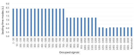
Figure 5. Example of sealing-time modes of grouped signals in shift 5 (isize = 50).

After determining the number of clusters in the shift, the algorithm must detect which intervals the mode changes occur between and thereby finally manage to determine the moment when the product change occurs. In the example we use as a basis to validate our proposal (shift 5), a first product change is detected between the clusters of 50 signals ranging from 701 to 750 and from 751 to 800. Consequently, it halves the $isize$ to adjust and determine where exactly the change occurs. The process would be the same in the other mode change (signals 1151–1200 and 1201–1250).

Reducing the interval size results in four clusters of 25 signals in which the mode is recalculated (see Figure 6). As can be observed, the mode change occurs between intervals 751–775 and 776–800.

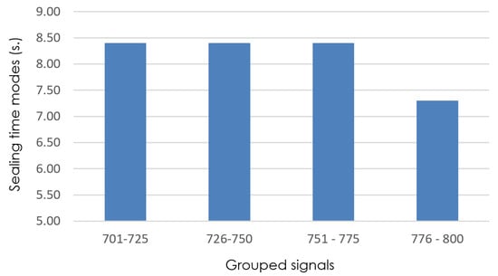
Figure 6. Detail of sealing-time modes (grouped signals 701–800), with isize = 25.

MoBiSea again halves $isize$ and recalculates the mode of the signals from 751 to 800. Figure 7 presents the result of this process, showing the modes of the analyzed intervals ($isize=12$). As can be seen, the algorithm detects that the product change occurs between signal clusters 763–775 and 776–787.

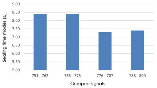
Figure 7. Detail of sealing-time modes (grouped signals 751–800), with isize = 12.

The process of reducing the interval sizes is repeated until $isize=1$ since that is when MoBiSea identifies exactly when the product change occurs in the manufacturing process. Figure 8, Figure 9, Figure 10 and Figure 11 show how sealing-time modes are recalculated to observe when a significant change occurs in their value and, therefore, to reduce the set of signals analyzed until this change is found.

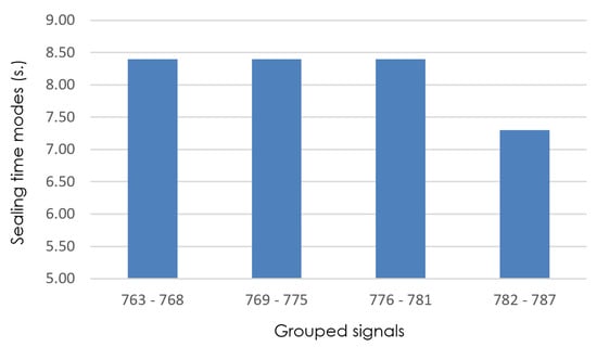
Figure 8. Detail of sealing-time modes (grouped signals 763–787), with isize = 6.

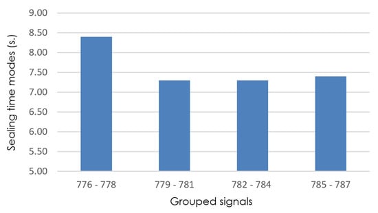
Figure 9. Detail of sealing-time modes (grouped signals 776–787), with isize = 3.

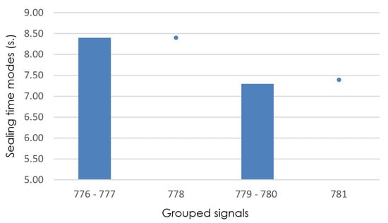
Figure 10. Detail of sealing-time modes (grouped signals 776–781), with isize = 2.

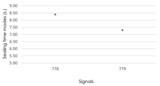
Figure 11. Detail of sealing-time modes (signals 778 and 779), with isize = 1.

Finally, Figure 12 and Figure 13 provide an overview of the sealing signals collected by the system and how the signals are grouped based on differing interval sizes. Figure 12 shows the sealing times for signals the device receives correctly in blue and wrong signals due to EMI in red. The signal analysis that makes it possible to detect product changes (in this case, whole cheeses, cheese quarters and cheese wedges) can also be observed. Specifically, one product change occurs at 15:30 and another one at 19:35.

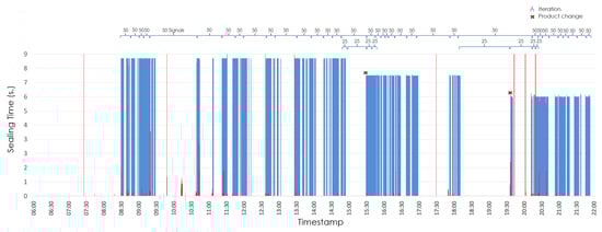
Figure 12. Example of all the signals gathered during shift 5.

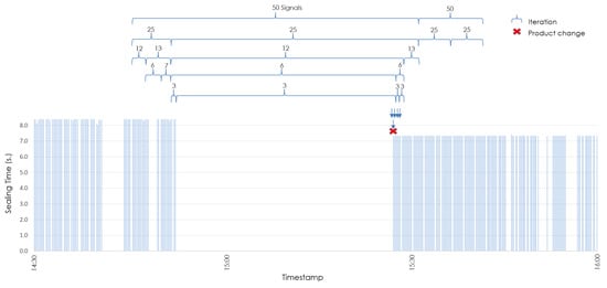
Figure 13. Details of product-change analysis.

Figure 13 shows details of how MoBiSea works to determine the exact point when the product change occurs between 14:30 and 16:00. Given that MoBiSea detects a mode change (i.e., the difference between them is more than the established $threshold$) between both clusters of 50 signals, these are divided into clusters of 25 signals, to determine between which of them a mode change again occurs. As mentioned above, the process is repeated until the exact signal at which the product change occurs is determined.

4. Comparison with Other Clustering Algorithms

We analyzed six different production shifts to check the performance of MoBiSea with respect to the clustering mechanisms presented above in Section 2 by comparing the values MoBiSea obtains with those obtained via x-means, k-means and k-rms. We also compared them with real data to check the values were correct and precise. The methods we refer to, k-means and x-means, enjoy wide recognition and use within what is referred to as clustering. For this reason, we have chosen to present them as a base that is familiar to the reader. However, in addition to comparing ourselves against classic algorithms, we have also compared our proposal against more recent approaches such as k-rms. Our goal is to establish a recognizable environment, thus facilitating a more nuanced understanding of the unique attributes and advances that our approach incorporates, as well as making a comparison with improved and current algorithms.

The first two metrics analyzed are the number of clusters detected by each algorithm and the position of the centroids.

It is important to note that both k-means and k-rms cannot determine the number of clusters by themselves since that value is a parameter that the user must establish. Therefore, the number of real clusters has been used for comparison purposes. With MoBiSea, the centroids are given by the mode value of the sealing times in each of the clusters.

The third metric to consider is the number of signals included in each of the clusters by each of the algorithms. These data are essential, since they show how many units have been made of each product during the shift.

Finally, since the aim is to learn the exact moment when the shift change occurs (necessary for the correct operation of the DBF filtering mechanism), the exact product start and end signals determining each of the algorithms need to be determined.

Considering this, Table 4, Table 5 and Table 6 show the data obtained from the metrics previously mentioned (i.e., the number of clusters, the position of the centroids, the number of signals of each product, as well as the start and end values of each cluster). In addition, the real values are presented, so that the errors committed by each of the analyzed mechanisms (i.e., k-means, x-means, k-rms and MoBiSea) can be measured.

Table 4. Comparison between real-data metrics (Clusters/Center) and the results obtained via x-means, k-means, k-rms and MoBiSea.

Shift	Clusters/CENTER
	Real	x-Means	k-Means	k-rms	MoBiSea
1	1/7.34	1/7.42	1/7.30	1/7.33	1/7.34
	-	1/7.27	-	-	-
	-	1/7.24	-	-	-
2	1/7.34	1/7.08	1/7.22	1/7.04	1/7.34
	2/8.38	-	2/8.22	2/7.79	2/8.38
	3/5.96	-	3/5.73	3/6.21	3/5.96
	4/8.38	-	4/7.55	4/7.26	4/8.38
3	1/8.29	1/8.34	1/8.36	1/8.33	1/8.29
	2/6.05	2/6.08	2/6.23	2/6.13	2/6.05
	3/7.34	3/7.23	3/7.21	3/7.23	3/7.34
	-	4/7.12	-	-	-
4	1/7.34	1/7.23	1/7.23	1/7.28	1/7.34
	2/8.38	2/8.26	2/8.26	2/8.25	2/8.38
5	1/8.38	1/7.54	1/8.49	1/8.39	1/8.38
	2/7.34	-	2/7.69	2/7.57	2/7.34
	3/6.05	-	3/6.18	3/6.17	3/6.05
6	1/5.96	1/5.93	1/5.93	1/5.93	1/5.96
	2/8.38	2/7.47	2/7.46	2/7.11	-
	3/7.34	3/7.36	3/7.35	3/7.36	2/7.34

Table 5. Comparison between real-data metrics (number of signals (error)) and the results obtained via x-means, k-means, k-rms and MoBiSea.

Shift	Number of Signals (Error)
	Real	x-Means	k-Means	k-rms	MoBiSea
1	2046	479 (76.59%)	2046 (0.00%)	2046 (0.00%)	2046 (0.00%)
	-	996	-	-	-
	-	571	-	-	-
2	771	2588 (235.67%)	735 (4.67%)	1056 (36.96%)	771 (0.00%)
	401	-	427 (6.48%)	537 (33.92%)	401 (0.00%)
	914	-	696 (23.85%)	485 (46.94%)	914 (0.00%)
	502	-	730 (45.42%)	510 (1.59%)	502 (0.00%)
3	533	533 (0.00%)	533 (0.00%)	533 (0.00%)	533 (0.00%)
	581	581 (0.00%)	677 (16.52%)	602 (3.62%)	581 (0.00%)
	696	497 (28.59%)	600 (13.79%)	675 (3.02%)	696 (0.00%)
	-	199	-	-	-
4	981	977 (0.41%)	977 (0.41%)	1002 (2.14%)	981 (0.00%)
	1235	1239 (0.33%)	1239 (0.33%)	1214 (1.70%)	1235 (0.00%)
5	778	1671 (114.78%)	525 (32.52%)	641 (17.61%)	778 (0.00%)
	444	-	697 (56.98%)	581 (30.85%)	444 (0.00%)
	449	-	449 (0.00%)	449 (0.00%)	449 (0.00%)
6	888	888 (0.00%)	888 (0.00%)	735 (17.23%)	888 (0.00%)
	30	505 (1583.33%)	505 (1583.33%)	658 (2093.33%)	-
	1116	641 (42.56%)	641 (42.56%)	641 (42.56%)	1146 (2.69%)

Table 6. Comparison between real-data metrics (Start/Finish) and the results obtained via x-means, k-means, k-rms and MoBiSea.

Shift	Start/Finish
	Real	x-Means	k-Means	k-rms	MoBiSea
1	1/2046	1/479	1/2046	1/2046	1/2046
	-	480/1475	-	-	-
	-	1476/2046	-	-	-
2	1/771	1/2588	1/735	1/1056	1/771
	772/1172	-	736/1162	1057/1593	772/1172
	1773/2086	-	1163/1858	1594/2078	1773/2086
	2087/2588	-	1859/2588	2079/2588	2087/2588
3	1/533	1/533	1/533	1/533	1/533
	534/1114	534/1114	534/1210	534/1135	534/1114
	1115/1810	1115/1611	1211/1810	1136/1810	1115/1810
	-	1612/1810	-	-	-
4	1/981	1/977	1/977	1/1002	1/981
	982/2216	978/2216	978/2216	1003/2216	982/2216
5	1/778	1/1671	1/525	1/641	1/778
	779/1222	-	526/1222	642/1222	779/1222
	1223/1671	-	1223/1671	1223/1671	1223/1671
6	1/888	1/888	1/888	1/735	1/888
	889/918	889/1393	889/1393	736/1393	-
	919/2034	1394/2034	1394/2034	1394/2034	889/2034

As can be observed, the number of clusters the x-means algorithm records differs considerably from the real-number clusters in four of the six analyzed shifts. Especially noteworthy are shifts 1, 2 and 5, in which x-means determines a number of clusters that differ significantly from the real number. Furthermore, it does not follow a pattern; in other words, x-means fails in returning the correct number of clusters, both over- and under-estimating this number. In all these cases, the number of clusters MoBiSea estimates fully matches the real values, except in shift six, in which MoBiSea only detects two clusters instead of three. This is due to the fact that, in that particular shift, only 30 units of one of the products were elaborated (an unusually low number). Note that, although the x-means detects three clusters, it fails when determining the number of signals of each product. In addition, regarding the centroids, we see how MoBiSea satisfactorily detects the sealing times of the different types of product that have been produced in all shifts, except in shift 6, where MoBiSea does not record the sealing time in cluster 2 due to the aforementioned reason.

Regarding the number of signals in each cluster, in other words, the number of sealing actions taking place for each of the manufactured product types, we find that, for x-means, errors mostly occur when a wrong number of clusters has been determined, as expected. However, it also correctly (or with a minimal error) estimates the number of signals in some clusters. With k-means, the error is very small in most of the shifts, although it is noticeable for shifts 2, 5 and especially 6. Specifically, the error made in shift 5 is 32.52% and 56.98% for the first two clusters; the error is even higher in shift 6, rising up to 1,583.33% for the second cluster.

In the case of k-rms, the most significant errors also occur in shifts 2, 5 and 6, with greater emphasis on the latter. In shift 2, cluster 3 presents an error of 46.94%, followed by cluster 1 with an error of 36.96%. In shift 5, the greatest error is in cluster 2 with an error of 30.85% and finally, cluster 2 in shift 6 presents an error of 2093.33%. These errors may be produced by the attempt to minimize the variance within the clusters and an outlier or noise can significantly increase the variance of a cluster.

Some of the values in Table 4, Table 5 and Table 6 are presented visually in Figure 14, Figure 15 and Figure 16. These figures help us observe the different clusters, their signals and the start and end moments of each of the various products, determined via the analyzed clustering methods.

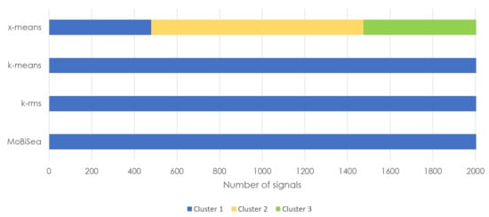
Figure 14. Products estimated via the x-means, k-means, k-rms and MoBiSea approaches in shift 1.

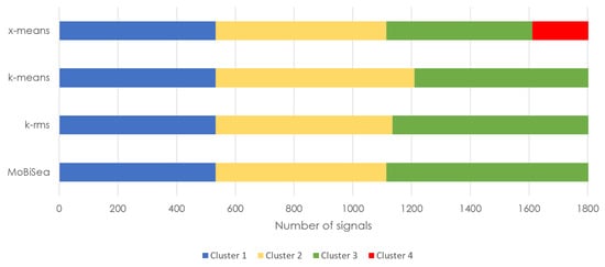
Figure 15. Products estimated via the x-means, k-means, k-rms and MoBiSea approaches in shift 3.

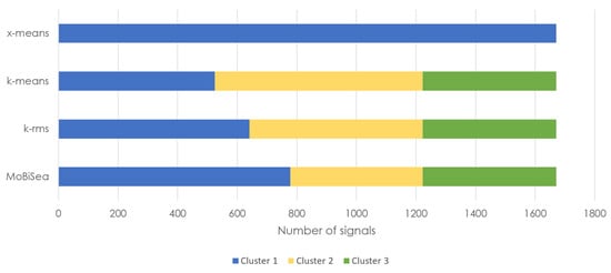
Figure 16. Products estimated via x-means, k-means, k-rms and MoBiSea approaches in shift 5.

Figure 14 shows how x-means erroneously determines that the number of different products made in shift 1 is three, while MoBiSea correctly determines that only one product was elaborated. Note that k-means and k-rms need to be manually provided with the number of clusters.

Similarly, Figure 15 shows the difference that exists between the four mechanisms, x-means, k-means, k-rms and MoBiSea, in terms of both cluster detection and the number of signals. In this case, the x-means mechanism determines four clusters in round 3, while MoBiSea accurately shows that three different types of products were manufactured. Regarding the number of signals for each product, all mechanisms correctly grouped the 533 units of the first product made, although k-means and k-rms make a mistake in determining the number of signals for the second and third clusters.

Finally, Figure 16 shows how x-means determines a single cluster for shift 5, while MoBiSea indicates that three different types of products were manufactured. Additionally, both k-means and k-rms incorrectly group the signals forming part of each of the clusters, especially for the first two products, although it is worth noting that k-rms comes closer to the actual signal grouping of the clusters.

5. Conclusions

When applied in industrial settings, the Internet of Things (IoT) changes how companies operate by facilitating and improving all production processes. However, proprietary systems in this type of setting usually involve high financial costs and this slows down adoption and, therefore, the transition to Industry 4.0. Nevertheless, there are more economical alternatives that, instead, rely on low-cost devices. Although these devices have similar features, their cost is much lower, which can undoubtedly accelerate technological transition in industry.

In this article, we have presented MoBiSea, an algorithm capable of determining the number of different product types made in each shift and also of determining the moments when their manufacturing process starts and ends. MoBiSea was created as a solution for our low-cost system for measuring OEE, which required operators to manually enter the details of the products made. Thanks to our mechanism, the OEE calculation system can work automatically without needing any operator intervention.

We compared MoBiSea with the results obtained via k-means, k-rms and x-means clustering algorithms, as well as with real values, to discover whether it performs correctly and precisely. We found that MoBiSea is completely accurate, since the values obtained exactly match the real values for all the shifts we studied, except for shift 6. We consider it negligible given its singularity. However, the data obtained via x-means, k-means and k-rms show wrong results, even though k-means and k-rms were previously provided with the correct number of clusters.

Specifically, k-means and k-rms have precision errors when determining the sealing times of the different products (shown by the cluster centroids); they also fail to correctly determine the number of seals for each product and the moments when the manufacturing of each product begins (start and end times). The error is more noticeable with x-means, since we have found that it does not correctly determine the number of products made in each shift; therefore, it does not determine the other parameters our system needs (sealing times, number of seals and start and end times of the product).

As future lines of research, we first intend to analyze how MoBiSea performs in other industrial production areas, since we consider that this algorithm can be used to identify and cluster products in other production lines.

In addition, as we want to estimate OEE in an unsupervised manner and, at this point, we can automatically quantify two of the three variables needed to determine OEE (i.e., availability and performance), we still have to solve the problem of obtaining data on the quality variable, since these data are currently entered manually. The time lost due to defective products will have to be determined for that purpose.

References

- Bajic, B.; Rikalovic, A.; Suzic, N.; Piuri, V. Industry 4.0 Implementation Challenges and Opportunities: A Managerial Perspective. IEEE Syst. J. 2021, 15, 546–559. [Google Scholar] [CrossRef]
- Horváth, D.; Szabó, R.Z. Driving forces and barriers of Industry 4.0: Do multinational and small and medium-sized companies have equal opportunities? Technol. Forecast. Soc. Chang. 2019, 146, 119–132. [Google Scholar]
- Nakajima, S. Introduction to TPM: Total Productive Maintenance; Productivity Press: New York, NY, USA, 1988. [Google Scholar]
- Herrero, A.C.; Martinez, F.J.; Garrido, P.; Sanguesa, J.A.; Calafate, C.T. An interference-resilient IIoT solution for measuring the effectiveness of industrial processes. In Proceedings of the 46th Annual Conference of the IEEE Industrial Electronics Society (IECON), Singapore, 18–21 October 2020; pp. 2155–2160. [Google Scholar] [CrossRef]
- Herrero, A.C.; Sanguesa, J.A.; Martinez, F.J.; Garrido, P.; Calafate, C.T. Mitigating Electromagnetic Noise When Using Low-Cost Devices in Industry 4.0. IEEE Access 2021, 9, 63267–63282. [Google Scholar] [CrossRef]
- Kaushik, S. An Introduction to Clustering and Different Methods of Clustering; Analytics Vidhya: Amsterdam, The Netherlands, 2016; p. 3. [Google Scholar]
- Duda, R.O.; Hart, P.E.; Stork, D.G. Pattern Classification and Scene Analysis; Wiley: New York, NY, USA, 1973; Volume 3. [Google Scholar]
- Bishop, C.M. Neural Networks for Pattern Recognition; Oxford University Press: Oxford, UK, 1995. [Google Scholar]
- Ishioka, T. Extended K-means with an Efficient Estimation of the Number of Clusters. In Proceedings of the Intelligent Data Engineering and Automated Learning-IDEAL 2000. Data Mining, Financial Engineering and Intelligent Agents: Second International Conference Shatin, NT, Hong Kong, China, 13–15 December 2000; Springer: Berlin/Heidelberg, Germany, 2003; p. 17. [Google Scholar]
- Rahamathunnisa, U.; Nallakaruppan, M.; Anith, A.; Kumar, K.S.S. Vegetable Disease Detection Using K-Means Clustering And SVM. In Proceedings of the 2020 6th International Conference on Advanced Computing and Communication Systems (ICACCS), Coimbatore, India, 6–7 March 2020; pp. 1308–1311. [Google Scholar] [CrossRef]
- Siswantoro, J.; Prabuwono, A.S.; Abdullah, A.; Idrus, B. Automatic image segmentation using Sobel operator and k-means clustering: A case study in volume measurement system for food products. In Proceedings of the International Conference on Science in Information Technology (ICSITech), Yogyakarta, Indonesia, 27–28 October 2015; pp. 13–18. [Google Scholar] [CrossRef]
- Hüseynli, A.; Yildiz, O.; Akcayol, M.A. Specification based automatic product categorization from unstructured data. In Proceedings of the 26th Signal Processing and Communications Applications Conference (SIU), Izmir, Turkey, 2–5 May 2018; pp. 1–4. [Google Scholar] [CrossRef]
- Hochdörffer, J.; Laule, C.; Lanza, G. Product variety management using data-mining methods—Reducing planning complexity by applying clustering analysis on product portfolios. In Proceedings of the IEEE International Conference on Industrial Engineering and Engineering Management (IEEM), Singapore, 10–13 December 2017; pp. 593–597. [Google Scholar] [CrossRef]
- Noorbehbahani, F.; Mansoori, S. A New Semi-Supervised Method for Network Traffic Classification Based on X-Means Clustering and Label Propagation. In Proceedings of the 2018 8th International Conference on Computer and Knowledge Engineering (ICCKE), Mashhad, Iran, 25–26 October 2018; pp. 120–125. [Google Scholar] [CrossRef]
- Garain, A.; Das, D. K-RMS Algorithm. Procedia Comput. Sci. 2020, 167, 113–120. [Google Scholar] [CrossRef]
- Imamura, K.; Kubo, N.; Hashimoto, H. Automatic moving object extraction using x-means clustering. In Proceedings of the 28th Picture Coding Symposium, Nagoya, Japan, 8–10 December 2010; pp. 246–249. [Google Scholar] [CrossRef]
- Knuth, D.E. The Art of Computer Programming, 2nd ed.; Addison-Wesley Longman Publishing Co.: Boston, MA, USA, 1998; Volume 3. [Google Scholar]
- Vuyyuru, G.M. KLP’s Search Algorithm—A New Approach to Reduce the Average Search Time in Binary Search. In Proceedings of the 4th International Conference on Electrical, Electronics, Communication, Computer Technologies and Optimization Techniques (ICEECCOT), Mysuru, India, 13–14 December 2019; pp. 185–190. [Google Scholar] [CrossRef]
- Jacob, A.E.; Ashodariya, N.; Dhongade, A. Hybrid search algorithm: Combined linear and binary-search algorithm. In Proceedings of the International Conference on Energy, Communication, Data Analytics and Soft Computing (ICECDS), Chennai, India, 1–2 August 2017; pp. 1543–1547. [Google Scholar] [CrossRef]
- Bai, Y.; Yang, L.; Zhang, G.; Xu, Y. An improved binary search RFID anti-collision algorithm. In Proceedings of the 12th International Conference on Computer Science and Education (ICCSE), Houston, TX, USA, 22–25 August 2017; pp. 435–439. [Google Scholar] [CrossRef]
Disclaimer/Publisher’s Note: The statements, opinions and data contained in all publications are solely those of the individual author(s) and contributor(s) and not of MDPI and/or the editor(s). MDPI and/or the editor(s) disclaim responsibility for any injury to people or property resulting from any ideas, methods, instructions or products referred to in the content. |
© 2023 by the authors. Licensee MDPI, Basel, Switzerland. This article is an open access article distributed under the terms and conditions of the Creative Commons Attribution (CC BY) license (https://creativecommons.org/licenses/by/4.0/).