1. Introduction
Hyperspectral images (HSI) are obtained and compiled using hyperspectral sensors or imaging spectrometers, which contain numerous continuous bands that offer abundant spectral and spatial information. As a result, hyperspectral images find valuable applications in mineral resources [
1], agricultural production [
2], environmental monitoring [
3,
4], and astronomy [
5]. Previous studies have employed various methods for hyperspectral image classification, as depicted in
Figure 1a, including Support Vector Machines (SVM) [
6], Random Forests (RF) [
7], sparse representation-based [
8] and K Nearest Neighbors (KNN) [
9]. However, these classification approaches are not well-suited for multi-classification problems and fail to effectively leverage the high-dimensional hyperspectral data. Consequently, they do not fully exploit the abundant spectral and spatial information available in hyperspectral images, leading to unsatisfactory classification results.
With the growing significance of deep learning in computer vision, deep-learning models exhibit greater network depth and enhanced data-mining capabilities compared to traditional network structures [
10]. In the realm of deep learning, various structural models have been applied to hyperspectral image classification, as illustrated in
Figure 1b, including Convolutional Neural Networks (CNN) [
11], Stacked Autoencoder Networks (SAN) [
12], Deep-Belief Networks (DBN) [
13], and Recurrent Neural Networks (RNN) [
14]. Among them, the Convolutional Neural Network (CNN) has emerged as the primary method for hyperspectral image classification. Yang et al. [
15] proposed a multilevel spectral–spatial transformation network (MSTNet) for hyperspectral image classification (HSIC). The network utilizes transformer encoders to learn feature representations and decoders to integrate multi-level features, resulting in accurate classification results. VGGNet [
16], introduced by Simonyan K et al., utilizes small convolutional kernels (3 × 3) and small pooling kernels (3 × 3), allowing for deeper network models while managing computational growth. ResNet [
17], also devised by He K M et al., enhances overall network performance through residual learning using convolutional layers and increased network depth. These advancements aim to improve the effectiveness of hyperspectral image classification. Zhu et al. [
18]. introduced a short-range and long-range graph convolution (SLGConv) based on the graph convolutional neural network. They utilized a three-layer SLGConv to construct the short- and long-range graph convolution network (SLGCN) for extracting both global and local spatial–spectral information to improve hyperspectral image classification. However, Liao et al. [
19] proposed a spectral–spatial fusion transformer network (S2FTNet) for HSI classification. S2FTNet leverages the transformer framework to create a spatial transformer module (SpaFormer) and a spectrum converter module (SpeFormer) to capture long-distance dependencies between image space and spectrum, enhancing the classification performance.
Although deep learning demonstrates excellent performance in hyperspectral image classification, its effectiveness heavily relies on a substantial number of labeled samples. Unfortunately, the process of labeling hyperspectral image samples is labor-intensive and costly, resulting in the limited availability of labeled data [
20].
The scarcity of labeled samples poses challenges such as overfitting the deep-learning model and reduced accuracy. Consequently, the primary focus of future hyperspectral image classification lies in achieving satisfactory results with limited samples. Finding ways to optimize deep-learning models under such circumstances is a key research direction in the field.
In recent years, few-shot learning has gained popularity and is commonly applied to few-shot target classification tasks. Two prominent approaches in few-shot learning are metric learning and meta learning, as depicted in
Figure 1c. Metric-learning methods focus on learning feature embeddings or similarity measures to enable classification based on discriminative similarities between query set labels and support set-labeled examples. These methods often employ episodic training mechanisms to acquire transferable knowledge. Meanwhile, the meta-learning method aims to learn an optimal initialization or optimizer that can generalize the model to unseen tasks. For instance, recurrent neural networks are employed to train cross-task meta-learners, enhancing knowledge transfers across different tasks and improving generalization performance. Both approaches share the common objective of learning a model capable of classifying query set labels with limited support set labels.
This paper combines various common classification methods for hyperspectral imagery with approaches used to address the issue of limited samples in traditional image processing. The main structure of this article is outlined as follows:
Related work: This section primarily focuses on presenting the relevant theories of metric learning and identifying the deficiencies in existing partial networks, subsequently leading to the introduction of the main innovations of our proposed network.
Materials and methods: We provide a concise overview of the designed network architecture, followed by a more detailed exposition of the concepts related to the spectral module, spatial module, and loss function.
Experimental results: This section encompasses the introduction of three commonly used hyperspectral image datasets, the description of the relevant experimental procedures, and a comprehensive analysis and discussion of the experimental results.
Conclusions: This section summarizes the main findings of the study, reviews the key points of the paper, and identifies the current limitations of the research, followed by proposing suggestions for future work.
3. Materials and Methods
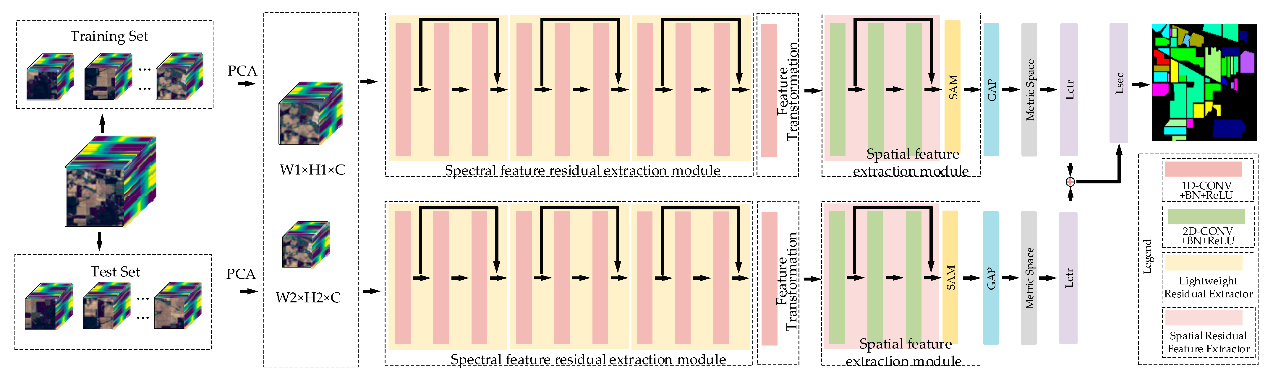
The network architecture of this study is depicted in
Figure 3. Initially, the hyperspectral image data samples are divided into a training set and test set. Each data sample is further segmented into data blocks of varying sizes, denoted as W1 × H1 for larger data blocks and W2 × H2 for smaller data blocks. During the training process, the data blocks of all samples are randomly selected and paired to create positive and negative sample pairs. These pairs are then input into the feature extraction network of the dual-channel Siamese network to extract deeper spectral and spatial information of hyperspectral data. The network model is continuously optimized through metric learning, which involves extracting feature vectors from hyperspectral image data. This enables the network to learn the classification ability for different classes. The parameters of the feature extraction module are adjusted via back-propagation of the loss function, facilitating the fine-tuning of the network.
During the testing process, the sample data in the test set is divided into a support set and a query set. The query set consists of the data to be detected, while the support set consists of the known class data. These two sets form a sample pair, where each pair is composed of a data block from the query set and a data block from the support set. The sample pairs are then input into the trained model. The trained model outputs feature vectors for each sample pair. The distance between the feature vector of the data in the query set and the feature vector of the data in the support set is calculated. The sample pair with the highest similarity in terms of feature vectors, specifically between the feature vectors of the support set and the query set, is selected. The predicted class for the data in the query set is determined based on this selected sample pair. This process completes the classification of hyperspectral images.
3.1. Model Method
3.1.1. Spectral Feature Residual Extraction Module
In the scenario of limited samples, the deep-learning network often encounters the issue of vanishing gradients as the number of network layers increases. To address this problem, the convolution residual method is incorporated into the spectral extraction module, which helps mitigate gradient degradation during the deepening of network. A lightweight implementation of the residual method is adopted. Each lightweight residual extractor, as depicted in
Figure 4, comprises convolutional layers, Batch Normalization (BN) layers, and ReLU layers, applied in sequence.
As illustrated in
Figure 4, the initial data input to the lightweight residual extractor is denoted as
. Each convolutional layer is subsequently followed by a Batch Norm layer [
31], facilitating network convergence and improving generalization ability. This data processing results in an output following a normal distribution with a mean value of 0 and a variance of 1. Furthermore, a Rectified Linear Unit (ReLU) activation function is employed to reduce network computational complexity and address the issue of gradient vanishing in deep network.
The spectral residual-extraction module is depicted in
Figure 5. In the first lightweight residual extractor, the convolution has a kernel size of 3 × 1 × 1 and 16 channels. For the second lightweight residual extractor, the convolution layer has a kernel size of 3 × 1 × 1 and 32 channels. The third lightweight residual extractor has a convolution layer with a kernel size of 3 × 1 × 1 and 64 channels. Additionally, the output of the first ReLU activation function
is added to the output of the third ReLU activation function,
, to obtain the overall output
. The computation process is shown in Equation (1). The output
is passed to the next lightweight residual extractor. The feature map obtained after extraction by three lightweight residual extractors is denoted as
.
Due to the limited number of samples in the few-shot scenario, it is important to control the number of parameters in the network model. Therefore, in the spectral feature-extraction part of the network, the special size of the three-dimensional convolution is set to 1, which effectively reduces the model parameters by 2/3.
The implementation of one-dimensional convolution in the network involves setting the spatial size of the three-dimensional convolution to 1, as shown in Equation (2). The value
of the one-dimensional convolution represents the computation of the neuron at position
in the
-th feature map of the
-th layer and is provided by the following equation:
where
represents the index of the feature map connected to the
-th feature map in the
-th layer,
is the size of the convolution kernel along with the spectrum dimension;
denotes the length of the spatial convolution kernel,
denotes the width of the spatial convolution kernel, and
and
are both set to 1;
is the value connected to the position
in the
-th feature map;
is the bias of the
-th feature map in the
-th layer; the function
is the ReLU activation function.
3.1.2. Spatial Feature Extraction Module
In scenarios of limited samples, effectively utilizing spatial information can significantly enhance hyperspectral image-classification capabilities. Based on the structural characteristics of HSI, this paper proposes a novel spatial feature extractor, depicted in
Figure 6. The spatial feature extractor primarily consists of a spatial residual feature extractor and a spatial attention mechanism.
Spatial Attention Mechanisms
The feature map
, obtained from the two-dimensional convolutional layer, serves as the input feature map of the spatial attention mechanism, as depicted in
Figure 7 below. Initially, the input feature map is fed into the spatial attention mechanism, where maximum pooling and average pooling operations are performed to capture different information. This result in two feature maps of
, each of size
, where every pixel in the generated image incorporates features from all channels at that position.
Then, the two generated feature maps
, both of size
, are then concatenated along the channel dimension. Subsequently, a 7 × 7 convolutional layer is applied to transform the feature map into a single-channel representation
of size
. The Sigmoid activation function is utilized to map the pixel values in the feature map to the probability space of 0 to 1, capturing the more prominent feature information in the image. This mapping generates spatial attention weight coefficients
. Finally, the attention weights are multiplied element-wise, channel-by-channel, with the input feature map of the module, denoted as “
× input features”, resulting in a new feature
of size
. The attention mechanism is expressed by Equation (4).
where
represents the attention weight coefficient,
represents the input feature,
represents the Sigmoid activation function,
represents the 7 × 7 convolution kernel, and AvgPool and MaxPool represent average pooling and maximum pooling respectively.
3.2. Loss Function
In the training process of the dual-channel Siamese network, the loss function is calculated using a weighted-comparison loss function and a label-smoothing cross-entropy loss function for each training iteration. The total loss function is expressed as Equation (5):
where
is the weighted contrast loss function, and
is the label-smoothing cross-entropy loss function.
The dual-channel Siamese network outputs two feature maps of different sizes,
and
, and extracts their center vectors,
and
, respectively, where
and
represent the sizes of two feature maps. The cosine distance
between two input sample pairs can be calculated using Equation (6), and the weighted comparison loss function is defined by Equation (7):
Equation (7) represents the weighted comparison loss function, where is multiplied by the positive sample pair, and is multiplied by the negative sample pair; denotes the distance between the feature vectors of the same class samples in a sample pair, while represents the distance between the feature vectors of different class samples in a sample pair. The variable represents the maximum distance between different samples.
The dual-channel Siamese network receives different information, resulting in a diversification of the output feature vector. To optimize the network parameters effectively, noise is introduced simultaneously to prevent excessive confidence in the correct label and enhance the network’s generalization ability. Hence, the label-smoothing cross-entropy loss function is introduced, defined by Equation (10) as follows:
In Equation (8), represents the probability of each category of data, corresponds to the weights associated with the -th category sample pairs, and is the vector of activations from the second-to-last layer of the network. denotes the transpose of .
In Equations (9) and (10), represents the label vector, is the label-smoothing factor, and represents the total number of categories being classified.
5. Conclusions
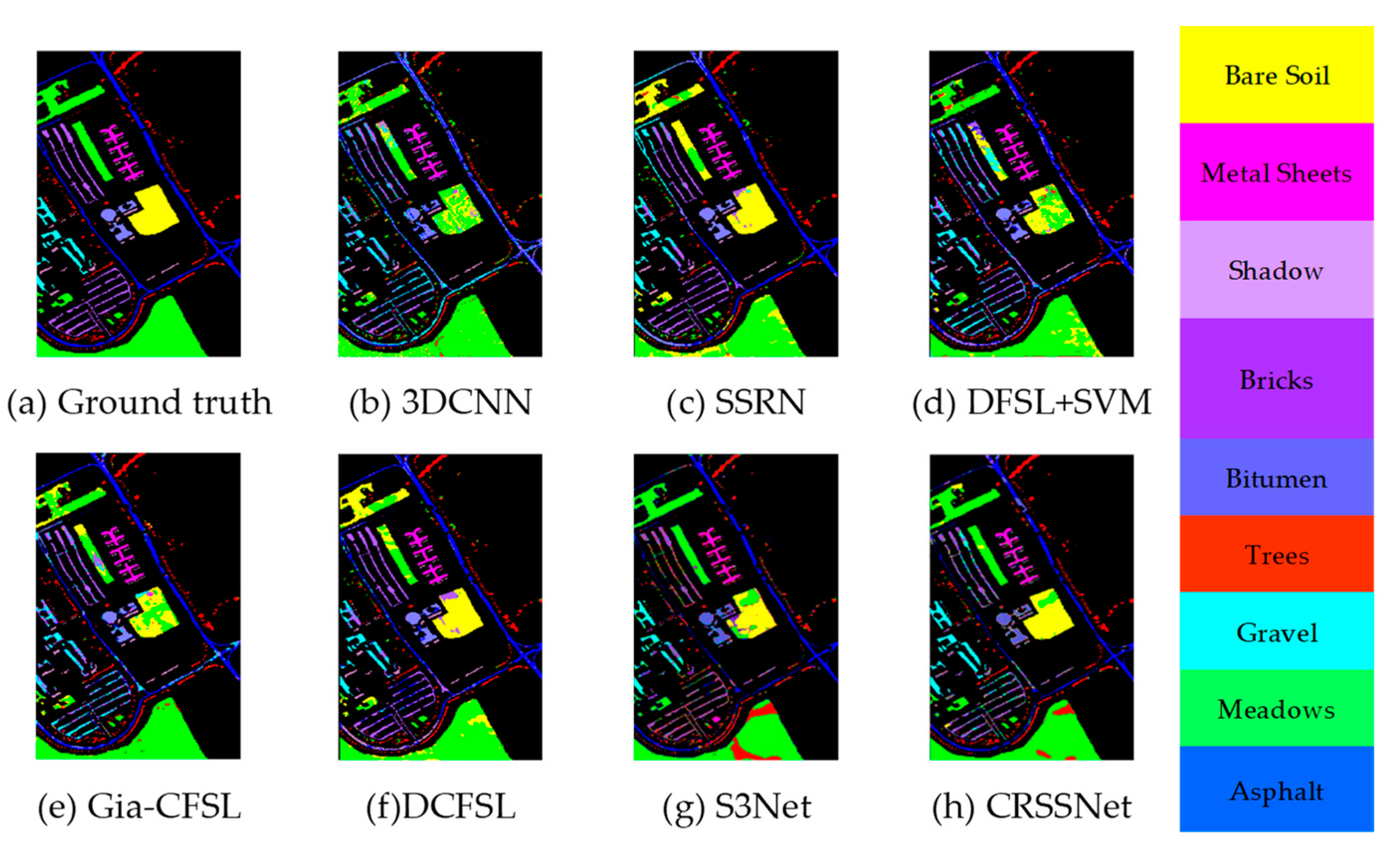
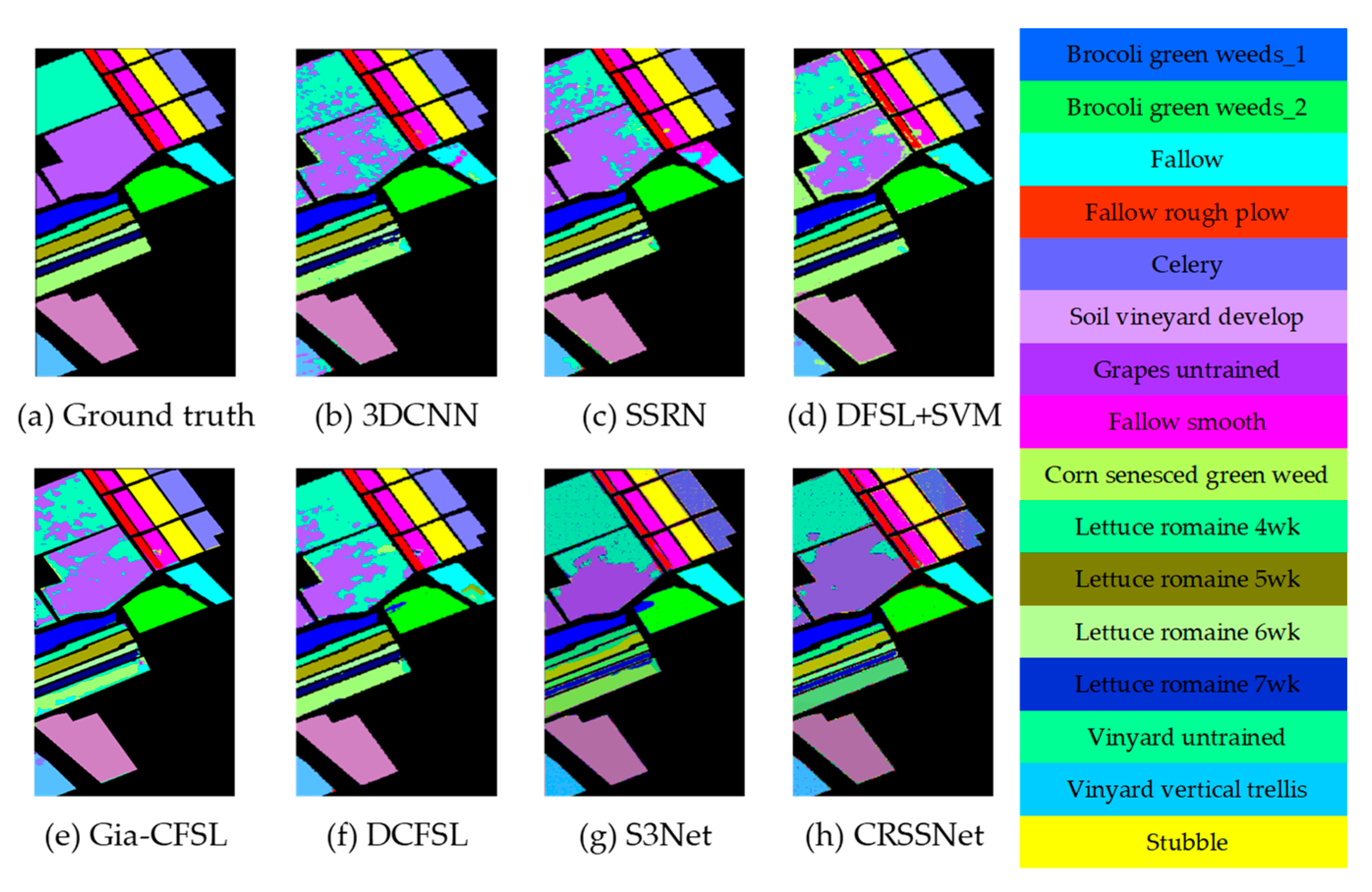
To address the challenges of insufficient spatial and spectral information extraction, as well as network overfitting in small-sample hyperspectral image classification, a method based on convolutional residuals and SAM Siamese networks is proposed. This method incorporates a feature residual-extraction module and a spatial attention mechanism to enhance feature information extraction. Furthermore, a more effective loss function is employed, which introduces noise and explores label factors to improve the classification capability of hyperspectral images with limited samples. Experimental results demonstrate the effectiveness of the proposed method on publicly available hyperspectral datasets, including Indian Pines, Pavia University, and Salinas. When compared to other methods, the proposed approach achieves superior classification performance in metrics such as OA, AA, and Kappa. These results highlight the method’s enhanced classification performance and improved generalization ability. However, there are still some challenges that need to be addressed. As observed from
Figure 11,
Figure 12 and
Figure 13, the classification accuracy is relatively low when dealing with similar categories.
Currently, there are still challenges in solving the classification of hyperspectral images with limited samples, especially regarding the inherent high-dimensional nature of such images. Although our proposed network incorporates PCA for dimensionality reduction, the issue of high dimensionality persists due to the oversampling of the spectral dimensions in hyperspectral images. Recently, some graph-based methods for dimensionality reduction of hyperspectral images have been proposed. For instance, Luo et al. [
38] introduced an Enhanced Hybrid Graph Discriminative Learning (EHGDL) based on hypergraphs, while Zhang et al. [
39] presented Multilayer Graph Spectral Analysis of Hyperspectral Images using Multilayer Graph Signal Processing (M–GSP), among others, which have shown promising results. In future research, it would be beneficial to explore and build upon these graph-based methods to achieve better dimensionality reduction performance in hyperspectral image classification tasks.
Moreover, despite the need for a limited number of labeled samples in hyperspectral image classification, the reliance on manual labeling for training remains crucial. Therefore, future research should explore the potential of conducting hyperspectral image classification without the dependence on labeled samples. Such developments hold significant promise in contributing to the field and its practical applications.


 ,
, 


