Abstract
This study addresses the challenges of limited fault samples, noise interference, and low accuracy in existing fault diagnosis methods for three-phase inverters under real acquisition conditions. To increase the number of samples, Wavelet Packet Decomposition (WPD) denoising and a Conditional Variational Auto-Encoder (CVAE) are used for sample enhancement based on the existing faulty samples. The resulting dataset is then normalized, pre-processed, and used to train an improved deep residual network (SE-ResNet18) fault diagnosis model with a channel attention mechanism. Results show that the augmented fault samples improve the diagnosis accuracy compared with the original samples. Furthermore, the SE-ResNet18 model achieves higher fault diagnosis accuracy with fewer iterations and faster convergence, indicating its effectiveness in accurately diagnosing inverter open-circuit faults across various sample situations.
1. Introduction
The three-phase inverter is a crucial conversion device in motor drive systems and is extensively utilized in various industrial control and power electronics fields. However, due to the large number of switch transistors and the high operating frequency of the three-phase inverter, the switch status undergoes high-frequency switching in a short period, leading to an increase in the failure rate of the switch transistors. Such failures disrupt the regular operation of the inverter and pose a significant risk to associated equipment and systems.
The operating conditions of the inverter system are extremely complex and changeable, and the probability of failure of power-switching transistors increases significantly due to factors such as aging [1]. Short circuits and open circuits are the main types of power-switching transistor failures. When a short circuit occurs in a power-switching transistor, the fault diagnosis can be done directly through hardware protection. However, for an open-circuit fault in a power-switching transistor, due to its slow response characteristics, the open-circuit fault of the inverter is difficult to diagnose directly by traditional diagnostic methods, and working under fault conditions for a long time can also cause secondary failures of the inverter switch transistors [2]. Therefore, in-depth research on the causes and types of open-circuit faults in three-phase inverters and the development of an efficient method for diagnosing power-switching transistor failures are of great theoretical and practical significance.
Quantitative techniques for diagnosing open-circuit faults in inverter power transistors are primarily categorized into analytical model-based methods and data-driven approaches. The latter is further subdivided into statistical analysis, which leverages principal component analysis and Bayesian theory; signal processing techniques, which utilize wavelet and spectral analysis; and artificial intelligence algorithms, which employ neural networks, support vector machines, and fuzzy mathematics, among others [3].
The analytical model-based approach requires the development of a mathematical model of the controlled system in order to perform fault diagnosis. While this method offers high accuracy, it can pose significant challenges when dealing with complex controlled system mechanisms, fluctuating model parameters, or scenarios where establishing a mathematical model is unfeasible.
In contrast, there has been increased interest in the fault diagnosis domain for the data-driven approach. It eliminates the need for creating mathematical models and instead focuses on analyzing output data for fault diagnosis. This approach is renowned for its efficiency, flexibility, and adaptability, attributes that have contributed to its growing popularity and usefulness in real-world applications.
In recent years, numerous researchers, both domestically and internationally, have conducted extensive research on inverter fault diagnosis. Among analytical model-based methods, Xu et al. [4] proposed an adaptive sliding-mode, observer-based open-circuit fault diagnosis method for single- and double-transistor faults in inverters. The method can simultaneously implement single-transistor and dual-transistor open-circuit fault diagnosis, providing fast and robust diagnosis without the need for additional sensors. Fan [5] developed a hybrid bonding graph model of the system using bonding graph theory. They combined this model with the degradation characteristics of the inverter system to analyze early faults. They derived global analytic redundancy relations and established the mathematical model of the system using the traversing path method. This method transforms the problem of fault parameter identification into an optimization problem for the objective function. Finally, the constructed function was subjected to a sparrow search algorithm. Li et al. [6] proposed a fast and accurate method for diagnosing open-circuit faults in brushless DC motor inverters. This method utilizes current path detection topology and a variation-based approach to efficiently identify and locate faults.
As computational power continues to advance, the data-driven approach has gained traction. This approach relies on data analysis, extraction, and modeling to facilitate accurate prediction and decision-making. Numerous studies have recognized the potential of artificial intelligence as a key player in this approach.
Several researchers have chosen Convolutional Neural Networks (CNNs) as their preferred tool for diagnosing inverter faults. Specifically, Shen et al. [7] and Yu et al. [8] have utilized CNNs to address different challenges, showcasing high accuracy rates and strong performance in various conditions, such as noisy and sparse data. At the same time, other research endeavors have concentrated on methodologies based on signal analysis and feature extraction. For instance, Xu et al. [9] developed a method focused on analyzing the filtered output line voltage of a three-phase inverter. Similarly, Zhu et al. [10] and Sun et al. [11] both proposed strategies focused on extracting specific characteristic parameters from different aspects of the inverter system. Additionally, several studies have combined various techniques for more comprehensive fault diagnosis. Yang et al. [12] combined the use of Fast Fourier Transform (FFT) with evolutionary neural networks, while Yan et al. [13] incorporated feature engineering with deep neural networks for fault diagnosis in specific motor drives.
In summary, these diverse research contributions underscore the potential and versatility of data-driven methodologies in the field of inverter fault diagnosis. But data-driven methods also face problems such as a scarcity of data samples and poor quality of data samples.
Addressing challenges in data-driven methods, such as difficulties in sample extraction or scarcity of data samples, several researchers have turned to data augmentation. Sun et al. [14] employed the Conditional Generative Adversarial Network (CGAN) for sample augmentation and CNN for fault diagnosis, effectively addressing sample imbalances. They demonstrated the superiority of CGAN compared with conventional methods such as the Synthetic Minority Over-Sampling Technique (SMOTE) and Generative Adversarial Network (GAN). Similarly, Cui et al. [15] proposed an enhancement to the AlexNet-based T-inverter open-circuit fault diagnosis using the Gramian Angular Field. This approach solves problems related to high fault feature similarity, manual extraction of fault features, and ineffective one-dimensional convolutional neural network feature extraction. It achieves this by converting one-dimensional signals into two-dimensional images. Lastly, Luczak et al. [16] addressed the issue of fault-tolerant control of three-phase inverters through hardware rewiring. Their method transforms three-phase currents into a single RGB image and applies convolutional neural networks for multiclass classification, effectively addressing fault detection and localization issues. Collectively, these studies demonstrate the significant potential of data augmentation in data-driven methods for inverter fault diagnosis.
Through an analysis of current domestic and foreign research, it is evident that researchers increasingly favor data-driven models for studying inverter faults due to the rapid development of various fault diagnosis methods. The difficulties in inverter fault diagnosis mainly lie in two aspects: how to effectively extract fault sample features and how to select a suitable fault diagnosis model to improve the accuracy rate. This paper focuses on data processing and model construction to optimize the diagnosis of open-circuit faults in inverters. We propose a method for diagnosing open-circuit faults in inverters based on the channel attention mechanism deep residual network. This method aims to address the challenges of feature extraction and model selection.
This paper proposes a method to denoise the samples using Wavelet Packet Decomposition (WPD) and enhance the data using a Conditional Variational Auto-Encoder (CVAE) model. Afterward, we construct an improved residual network with a channel attention module (SE-ResNet18). Through comparative experiments, we found that data augmentation improved the accuracy of fault diagnosis on the dataset. We used the SE-ResNet18 model as the fault diagnosis model, demonstrating good performance in accuracy and iteration speed.
The main contributions of this paper are as follows:
- Utilizing a CVAE model, we extract latent information from the original samples in order and generate new samples to augment the number of samples.
- To leverage the superior feature extraction capability of convolutional neural networks (CNNs), we employ a sample normalization technique to convert the sample data into 2D grayscale images. This approach offers a novel method for processing inverter sample.
- We introduce a channel attention mechanism into a deep residual network to improve the extraction of fault features. This method achieves higher accuracy and faster model convergence compared to the residual network.
The organization of the paper can be summarized as follows: Section 2 describes the research background on three-phase inverters and reviews the existing fault diagnosis methods. Section 3 introduces the category and processing method of inverter fault data collected in this paper, as well as the fault diagnosis model with the channel attention mechanism. Section 4 covers data augmentation and fault diagnosis experiments, described in detail. Finally, the conclusion is presented in Section 5.
2. Deep Residual Network
A Convolutional Neural Network (CNN) is a sophisticated deep learning model primarily used for processing structured grid data, such as images [17]. It consists of a sequence of convolutional, activation, and fully connected layers, where each layer is a differentiable non-linear module that is trained in an end-to-end manner. However, as the network depth increases, CNNs may encounter vanishing or exploding gradient issues, which can potentially result in network convergence failure.
Addressing these issues, He et al. [18] proposed the Deep Residual Network (ResNet), which utilizes a novel residual block structure. This structure forms shortcut connections, linking the input signal to subsequent weighted layers, and bypasses the information from the intermediate layers. This effectively mitigates the issues of vanishing and exploding gradients, thereby enhancing the training effectiveness of the deep neural network. The key aspect of the residual block structure is that it allows the network to learn the residual function, which captures the difference between the input and output of the block. By incorporating this residual function into the input, the network can efficiently learn the identity function. This ensures that useful features can still be learned, even when the network has numerous layers.
Hence, the key distinction between CNN and ResNet is architectural. While a CNN is a traditional multi-layered neural network that may suffer from performance degradation due to vanishing or exploding gradient issues, a ResNet effectively circumvents these issues with its innovative residual block and shortcut connection design. This allows for a deeper level of network training. Furthermore, the capability of ResNet to learn the residuals between inputs and outputs enhances the performance and training efficiency of the model. This is one of the rationales for adopting ResNet as the base model in this study.
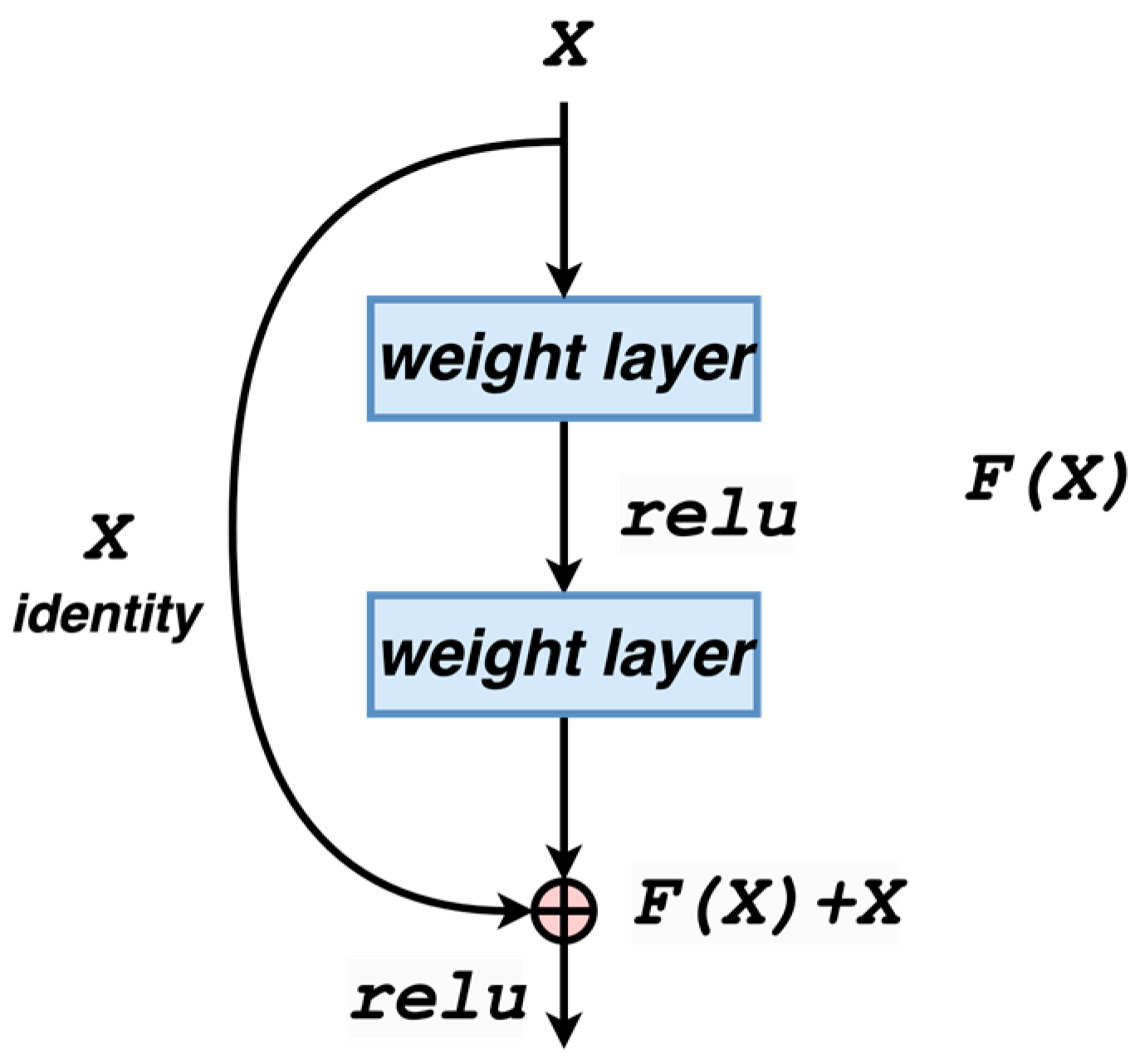
Figure 1 shows the ResNet residual module, which utilizes a shortcut connection to transfer the input across layers and then add it to the result after a convolution operation. In this module, is the input, and is the output. The output after intermediate convolution is a deformed expression of , and the final output is obtained as . The residual function is more accessible to optimize than the direct . The input is connected across layers with the obtained by stacking the weight layers, and the output of the residual module is . The calculation of residuals is more straightforward than the standard calculation, and the residuals will be significantly less challenging for a smaller dataset. Therefore, this paper uses the residual network as the base model. The calculation of the residual unit can be expressed using Equations (1) and (2):
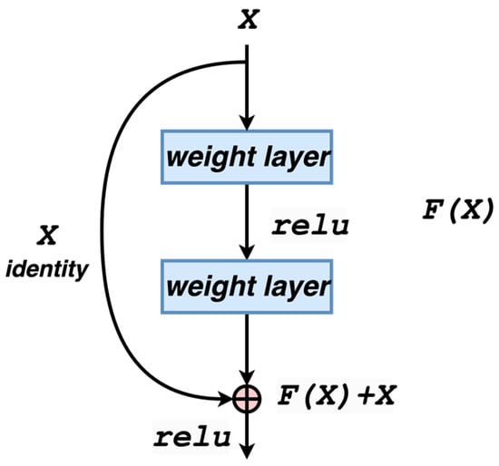
Figure 1.
Residual structure.
In Equation (1), and denote the input and output of the corresponding residual units, and F represents the learned residuals. In Equation (2), denotes the constant mapping, and is the nonlinear activation function. The process of feature learning from shallow to deep layers is illustrated in Equation (3):
3. The Proposed Method
3.1. Research Method
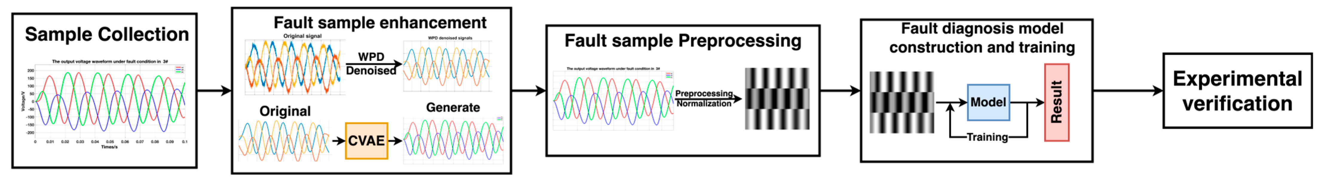
The fault diagnosis method proposed in this pape, as shown in Figure 2, consists of five stages. The first stage involves collecting actual fault data from the three-phase inverter sampling. However, we encountered two issues with the collected fault samples. Firstly, the limited number of samples made it challenging to train a model with a high diagnostic performance. Secondly, some of the collected samples had noise issues during the collection process, which can impact accuracy of the fault diagnosis in later stages. To address these issues, we enhanced the acquired data using fault sample enhancement techniques.
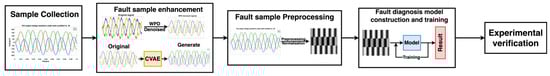
Figure 2.
Research methodology Schematic.
To address the issue of the small sample size, the proposed method utilizes a CVAE model to extract latent information from the existing samples and generate additional samples. Furthermore, the fault samples are denoised using the WPD method. Denoising helps to mitigate the impact of noise on the accuracy of the model and accelerates the convergence speed of the model. In the preprocessing stage, the three-phase data sequences in the fault data file are horizontally concatenated to form a two-dimensional matrix. The matrix elements are then normalized to the range of [−1, 1] and converted into grayscale images. This facilitates feature extraction by the CNN model, as it is based on the normalized values of the images.
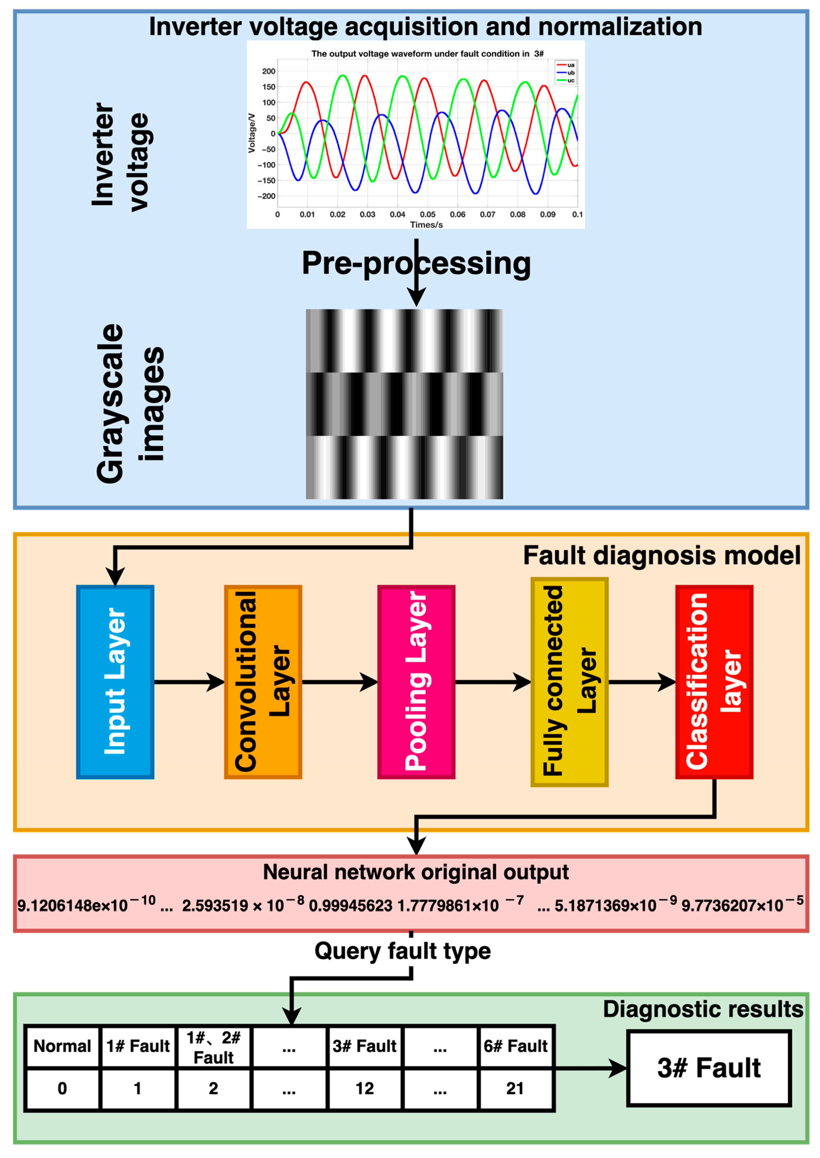
Based on the characteristics of the preprocessed samples, we constructed and trained an improved deep residual network. The processed fault samples were input into the trained model, and the network’s original output was a 22-dimensional vector. We extracted the index of the maximum value in the vector to obtain the corresponding fault label. Finally, we utilized the received fault label to retrieve the fault category from Table 1 and ascertain the diagnostic result by considering the open-circuit fault type. It should be noted that in Table 1, 1#–6# represent the transistor numbers in the three-phase inverter. This process concludes completing the fault diagnosis. Figure 3 illustrates the fault diagnosis process in this article.

Table 1.
Open-circuit fault types.

Figure 3.
Fault diagnosis flow chart.
3.2. Fault Sample Processing
3.2.1. Failure Mode Analysis
Open-circuit faults in three-phase inverters can be categorized into two types: those caused by external factors and those caused by internal factors. External factors include unstable supply voltage, environmental pollution, and high temperature, while internal factors consist of component aging, design defects, and circuit faults. Common open-circuit faults in three-phase inverters include IGBT failures, capacitor failures, disturbances, and insulation fractures. IGBTs are crucial for energy conversion and transmission and are widely used in power transmission, electric vehicles, and traction applications. They can efficiently convert electrical energy into mechanical or thermal energy with minimal loss.
IGBT failure is the most common type of open-circuit fault, often caused by internal structural damage or overvoltage/overcurrent from the power supply. Three-phase inverters typically contain six switching transistors, each controlling the current polarity of one load terminal in the circuit to provide control over three-phase AC power. In practical industrial applications, it is unlikely that all three switching transistors will fail simultaneously. Therefore, in this study, we assume that no more than two IGBTs will fail simultaneously, allowing us to classify open-circuit faults into five categories:
- Normal;
- Single-transistor failure;
- Two power transistors failures in a cross-half bridge;
- Two power transistors failures in a single-phase bridge;
- Two power transistors failures in the same half bridge.
This article categorizes the two power transistors failures as double-transistor open-circuit faults, resulting in three categories of open-circuit faults in this article: no fault, single-transistor open-circuit fault, and double-transistor open-circuit fault. Table 1 shows the fault categories.
3.2.2. Fault Sample Enhancement
Acquiring fault data for three-phase inverters involves observing and recording changes in the operational state parameters of inverters with open-circuit faults for each respective fault category. Multiple experimental samples were collected for each type of fault to ensure the reliability of the data. The data used in this paper were obtained by simulating various operating conditions and adjusting parameters, such as load size and input voltage. The dataset includes normal samples and 21 categories of fault samples across 25 different operating conditions. These conditions involve varying input voltage (500 V, 520 V, 540 V, 560 V, 580 V) and load power (40 kw, 45 kw, 50 kw, 55 kw, 60 kw).
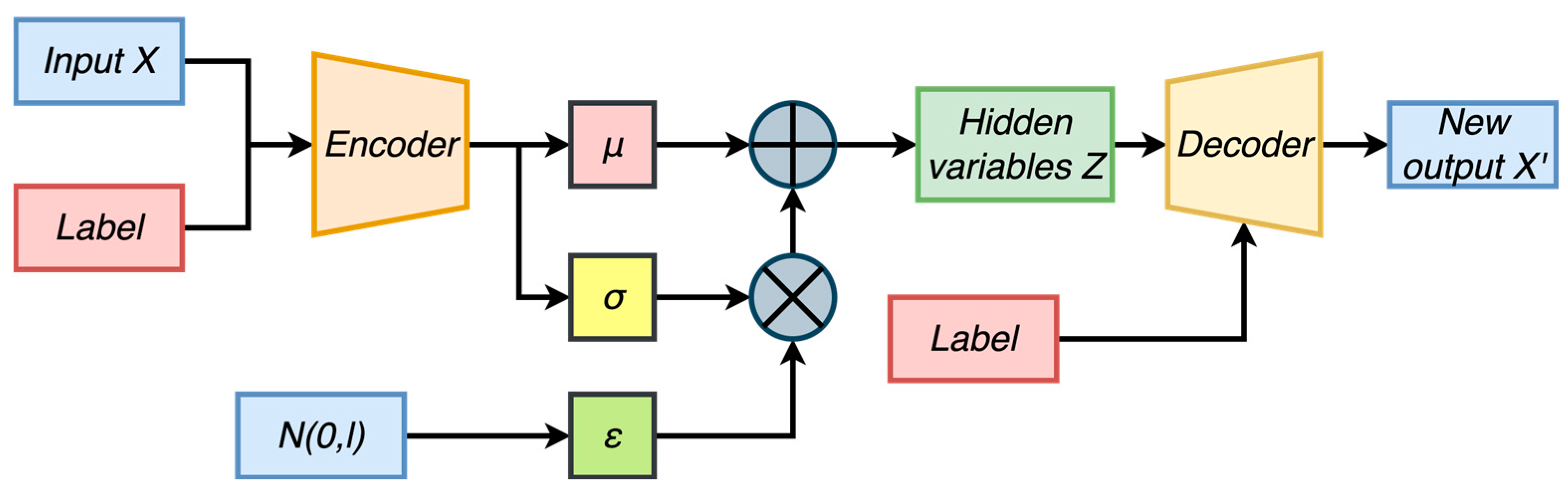
To enhance the diversity of the dataset and uncover latent features within the samples, we utilized a Conditional Variational Autoencoder (CVAE) for data augmentation. The Variational Autoencoder (VAE) is a generative neural network structure based on the Variational Bayes inference proposed by Kingma et al. [19]. The main concept of VAE is to utilize an encoder to map input data to the latent space and a decoder to sample and generate data from the latent space. CVAE introduces conditional variables to control the generation process and achieve specific outputs. It describes observations in the latent space probabilistically and has significant value in data generation applications. In the VAE model, the original data is input into the encoder to obtain the variational probability distribution of the hidden variable . This involves obtaining the mean and variance of the distribution. Resampled data, based on the variational probability distribution of the hidden variable is input into the decoder to receive the generated that approximates the original data . The optimization objective of VAE is shown in Equation (4):
In Equation (4), represents the KL divergence, represents the prior distribution, which is generally set as a standard normal distribution , and represents the exclusive posterior distribution of . For each input data , a corresponding latent distribution exists, i.e., an exclusive posterior distribution based on input data. represents the expectation of under the distribution . The first part of the equation is a constraint term that improves the diversity of the latent variables, and the second part is a reconstruction term that ensures the accuracy of the reconstruction.
The optimization objective of CVAE is shown in Equation (5), where represents the original data, represents the category label, and represents the latent variable.
We used CVAE to generate inverter fault data by category and concatenate the actual fault data and its corresponding label into a vector and input them into an encoder consisting of fully connected layers. The encoder compressed the original data into a low-dimensional space, mapping the visible variables to continuous latent variables. We used two independent fully connected layers with linear activation functions to generate the mean and standard deviation of the latent variable . We then deduced using the reparameterization trick. The label and were sent into the decoder to obtain new output with the same category as the label. The CVAE model structure used in this article is shown in Figure 4:
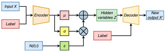
Figure 4.
Conditional variational auto-encoder.
Despite the presence of noise in our samples, we prioritized the authenticity of the experimental data. We chose to use an enhancement followed by a processing approach. This strategy maximizes the proximity of the processed samples to the original ones, preserving their inherent features to the greatest extent possible. This method enables us to extract the implicit characteristics of the original samples, ensuring both reliability and validity in our research.
Although CVAE increased the number of samples, the existing data still contain noise, which can lead to ineffective diagnosis by subsequent models. Therefore, we processed the noisy samples using the WPD to enhance the data.
3.2.3. Wavelet Packet Decomposition Denoising
To overcome the limitation of wavelet analysis, which only focuses on the low-frequency part of signals and does not process high-frequency components, Wickerhauser et al. proposed the theory of the Wavelet Packet Transform. The Wavelet Packet Transform [20] inherits the characteristics of wavelet analysis, allowing for the effective decomposition of both the low-frequency and high-frequency components of signals. This ensures that the frequency content of signals is preserved.
For a given orthogonal scaling function and its corresponding wavelet function, the bi-scale equation can be expressed as Equations (6) and (7):
In Equation (6), denotes the index of the function. When = 0, and . Here, represents the scaling function, and represents the wavelet mother function. The set of functions determined by the above equation is known as the wavelet packet determined by the scaling function . Thus, the wavelet packet is a collection of functions that includes both the scaling function and the mother wavelet function and has a certain intrinsic relationship between them.
The WPD algorithm is a generalization of the Mallat wavelet fast algorithm, and it can be expressed as Equation (8):
The second step of the WPD denoising algorithm is to select an appropriate threshold value. When the threshold value is too small, it is not possible to remove the noise signal from the mixed signal. When the threshold value is too large, it will eliminate a portion of the original signal and result in the absence of the original signal. Therefore, both the noise and the original signal should be considered comprehensively when estimating the threshold and selecting an appropriate threshold value. The threshold estimation is expressed as shown in Equation (9):
Here, is the threshold value, denotes the standard deviation of the noise signal, and is the length of the signal. The equation shows that the threshold value is selected proportionally to the noise’s standard deviation and the signal’s size. When the standard deviation of the noise signal increases, a higher threshold value is required to effectively suppress the noise interference. When the standard deviation of the noise signal decreases, a smaller threshold is necessary to preserve the original signal and prevent its suppression.
After selecting an appropriate threshold, the threshold function must process the wavelet packet coefficients that are more significant and less significant, and ultimately obtain the new denoised wavelet packet coefficients. In this paper, we have chosen to use the soft thresholding method for decomposing the thresholds. The specific expression of the soft thresholding method is shown in Equation (10):
where , represent the coefficient of the k-th point in the jth layer, and represents the threshold value. After the coefficients are thresholded, the wavelet packet reconstruction is performed using the reconstruction algorithm in Equation (11):
When the inverter sample contains noise, it can be described as , where represents the original inverter voltage signal, and represents the noise mixed in. When is wavelet transformed, and produce differences in energy distribution, with being more concentrated in the whole signal and more dispersed in the signal. Therefore, a suitable energy value can be found as the threshold value, and the appropriate threshold function is used to process the decomposition coefficients to obtain a new series of decomposition coefficients. The new decomposition coefficients can suppress the signal and retain the signal. Then the wavelet packet inversion transformation is carried out on the decomposition signal according to the brand new decomposition coefficients to derive the denoised signal. This way, the wavelet packet transformation can be used to achieve the effect of signal noise reduction. The specific wavelet packet denoising process is shown in Figure 5.

Figure 5.
WPD denoising process.
The WPD method offers substantial advantages in mitigating noise in real-world three-phase current signals. WPD enables a detailed, multi-resolution analysis across multiple frequency scales, which is essential for processing signals with diverse frequency components. Importantly, it reduces noise while preserving the crucial characteristics of the original signal, such as spikes and edges. This greatly aids in the subsequent analysis of the signal and enhances the understanding of its physical significance. While conventional filters may have some noise reduction capability, WPD typically achieves superior results, especially for real-world three-phase current signals. Given these unique advantages, the application of WPD becomes critically necessary for processing such signals.
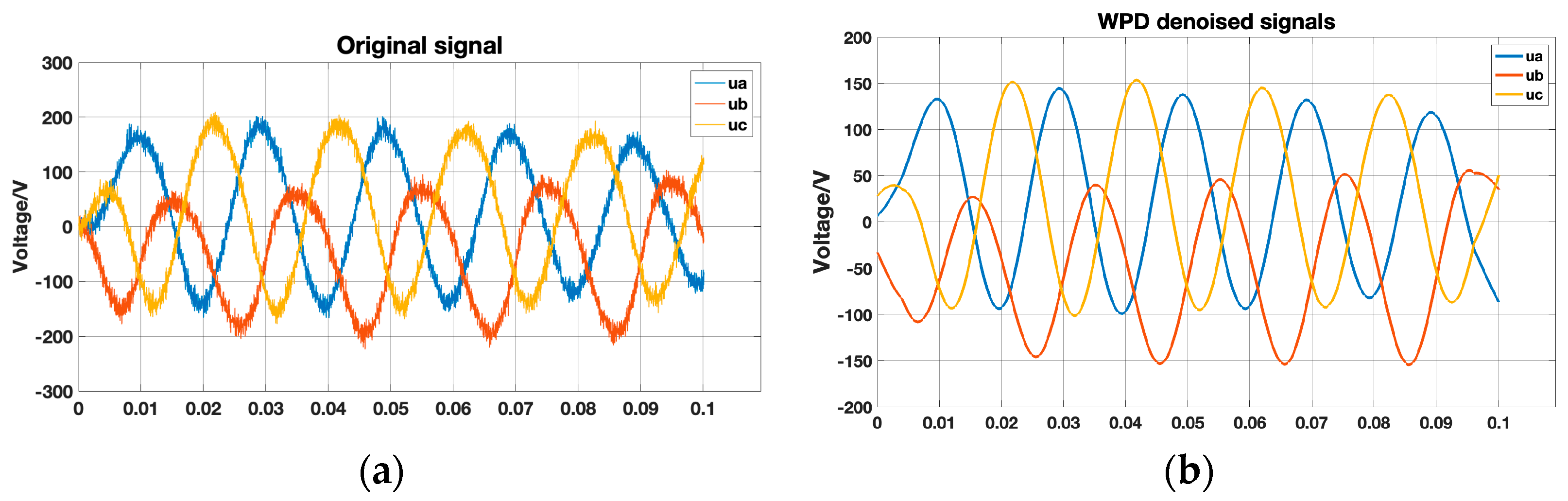
Figure 6 shows the original sample containing noise and the sample after denoising using WPD. The reconstructed signal obtained after denoising effectively removes the noise while preserving the valuable information in the original signal.

Figure 6.
Original and denoised samples. (a) Origin noise samples; (b) WPD denoised samples.
The importance of denoising cannot be ignored in the existing fault samples, although it is possible to distinguish the fault modes to some extent. Denoising can reveal the key characteristics of the signal and eliminate the ambiguity and misinterpretation caused by noise. It also helps to improve the robustness and generalization ability of the model, allowing it to maintain performance under different noise characteristics. Finally, this approach improves the accuracy and efficiency of subsequent processing steps, such as feature extraction or pattern recognition. It also reduces noise-induced interference and ensures the reliability of the results. Therefore, we strongly believe that denoising is a critical and necessary preprocessing step that helps to ensure the accuracy of the analysis results, improve the generalization ability of the model, and optimize the effectiveness of the subsequent processing steps.
3.2.4. Faulty Sample Preprocessing
After denoising the samples, we propose to preprocess the enhanced samples by converting the one-dimensional signals into two-dimensional grayscale images. This allows the model to extract detailed information about the local differences of the three-phase voltages, including many fault details. Next, the suitable fault feature extraction model should be selected based on the processed fault sample types for the fault diagnosis work.
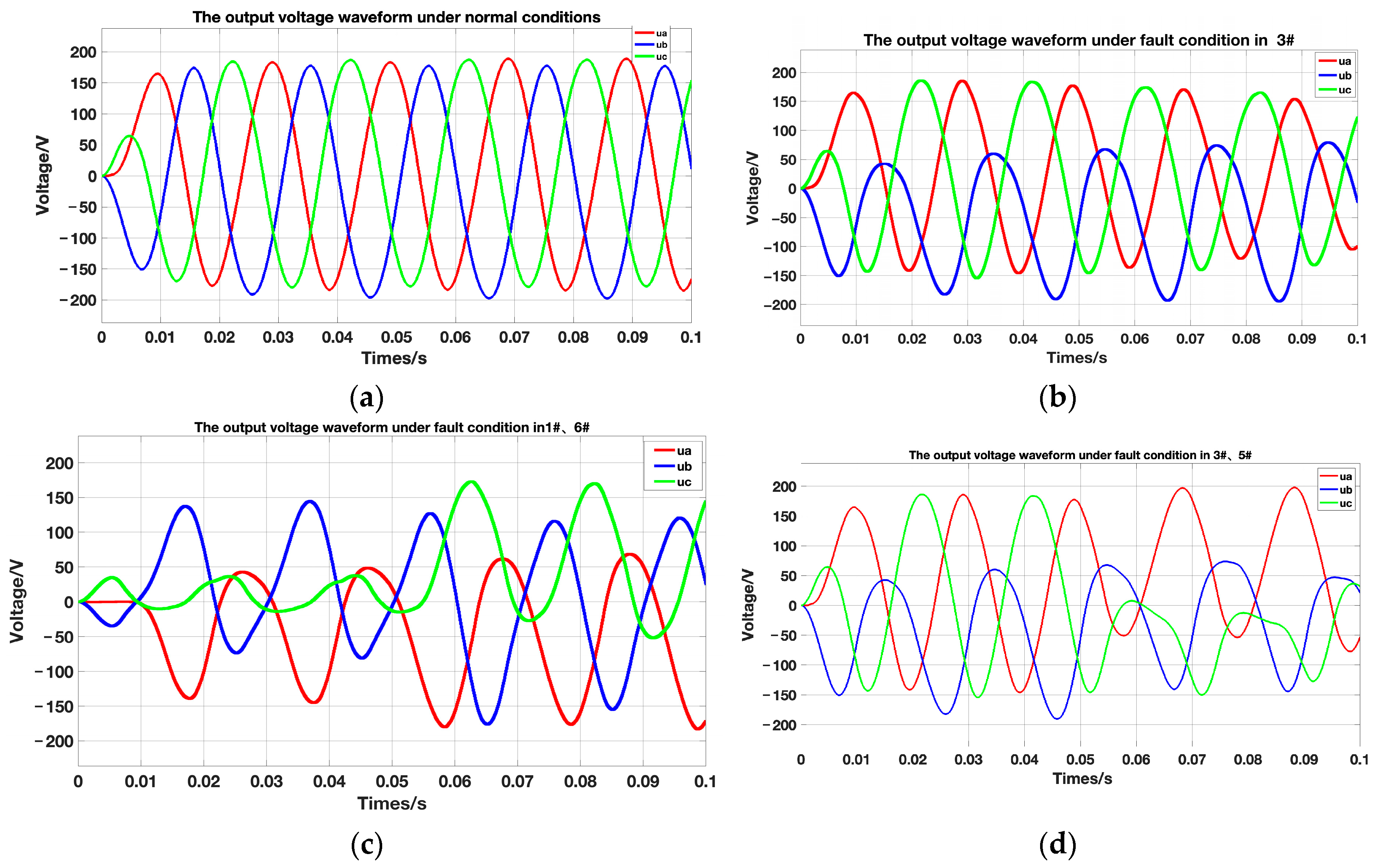
The next step is to preprocess the existing fault dataset in order to convert the data into a format that is suitable for convolutional neural networks. This can enhance the efficiency of fault diagnosis. First, the current fault dataset is visualized and analyzed. Figure 7 shows the output voltage waveforms for normal conditions and three open-circuit fault output voltage waveforms.
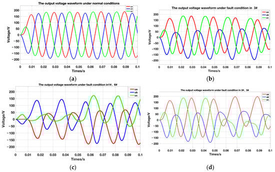
Figure 7.
Normal and open-circuit fault output voltage waveforms. (a) Normal-condition output voltage waveform; (b) 3# open-circuit fault output voltage waveform; (c) 1#, 6# open-circuit fault output voltage waveform; (d) 3#, 5# open-circuit fault output voltage waveform.
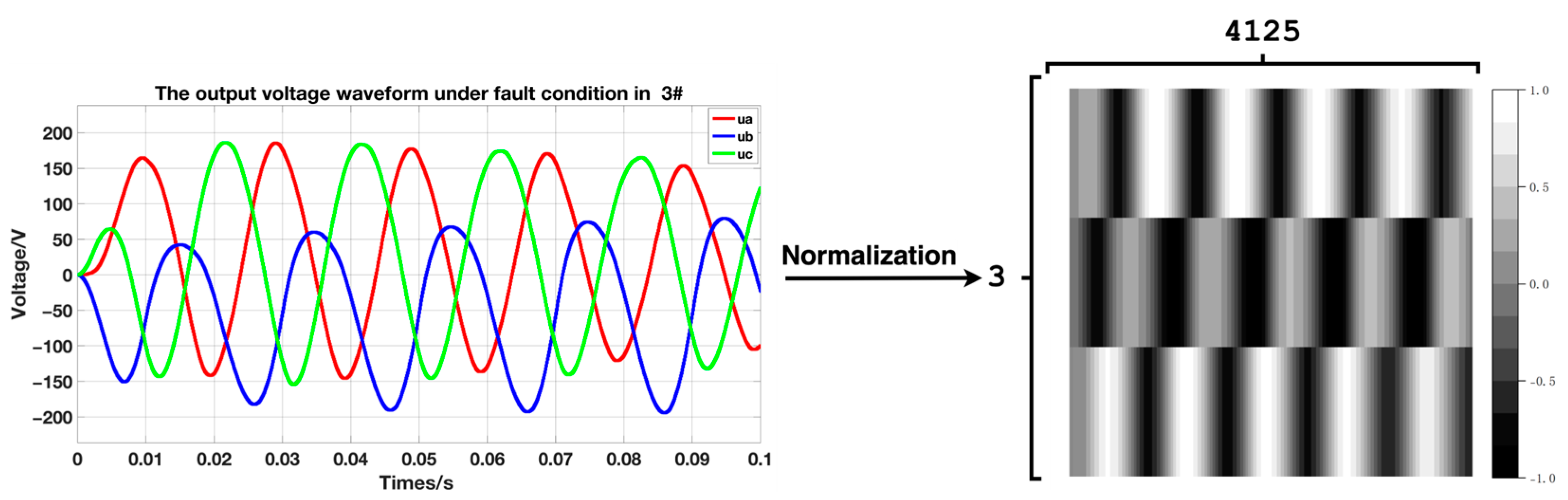
The 21 fault types and normal data obtained under 25 operating conditions are processed, along with five input voltages, five load power mixes, and the data generated by CVAE. The data-processing process is shown in Figure 8 and Figure 9. Firstly, the three-phase data sequences in the fault data file are combined into a two-dimensional matrix. This step is important for the convolutional neural network to extract a large amount of fault detail information from the local differences of the three-phase voltage through convolutional extraction. Then, the matrix elements are normalized to the range of [−1, 1], which is beneficial for avoiding numerical problems such as small network weights and neuron saturation. This normalization approach accelerates network training convergence and improves the network’s generalization ability in the presence of changes in operating conditions. After pre-processing, a single sample can be approximated as a grayscale image with L × 3 pixels, where L represents is the number of single-phase sampling points that correspond to the duration of the sample. In this experiment, the value of L is 4125.

Figure 8.
Fault sample preprocessing process.

Figure 9.
3# Fault output voltage data preprocessing schematic.
3.3. Fault Diagnosis Model Based on a Deep Residual Network
3.3.1. Channel Attention Module
The channel attention mechanism is widely used in convolutional neural networks for image-related tasks, including image classification, target detection, and image generation. The primary goal of this mechanism is to enhance the performance of the model by adjusting the weights of various feature channels. This enables the network to better focus on the relevant features for the given task, resulting in improved accuracy and performance. Each pixel in three-channel images has three values, so the channel attention mechanism must consider all three channels simultaneously. This increases the computational effort and complexity of the model. However, each pixel has only one value in grayscale images, so the channel attention mechanism only needs to consider one channel. This significantly reduces the computational cost and time overhead of the model, making it more efficient for processing grayscale images.
The fault diagnosis model chosen for this paper is the SE-ResNet18 model, which combines a compression-excitation network (SENet) module based on the channel attention mechanism with a deep residual network (ResNet). This model utilizes ResNet18 as the backbone network, which has a reduced number of layers. It enhances accuracy and performance by incorporating the SE (Squeeze-Excitation) [21] module between the convolutional layers. The SE module enables information interaction between channels, enhancing the network’s ability to extract and emphasize relevant features. The structure of the SE module is shown in Figure 10.
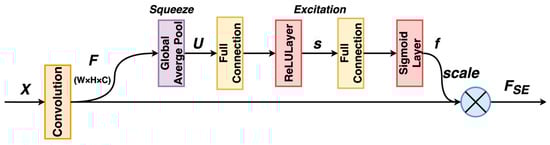
Figure 10.
SE module.
In the figure, the original sample’s dimension is , where denotes the number of channels, and and represent the height and width of the feature map, respectively. For a set of input features , the Squeeze operation obtains a global channel-dependent feature vector by averaging the pooling of features. The compression operation then reduces the dimensionality of the feature vector, compressing the spatial dimensions into one dimension. This results in a global field of view of the previous , making the perceptual area wider. Equation (12) demonstrates this process:
The Excitation operation’s primary goal is to calculate channel attention weights based on the global channel-related information obtained by the Squeeze operation and apply them to the channel dimensions of the input features for weighting. This operation consists of two steps: feature mapping and channel weighting. The first step is feature mapping, which maps the input feature to an intermediate node , where denotes the adjustable scaling factor. The mapping process is shown in Equation (13):
and denote the two learnable weight matrices for feature mapping, and represents the ReLU activation function. The second step is the channel weighting operation, which calculates the channel attention weight based on the features of the intermediate node and applies it to the channel dimension of the input features for weighting. The channel attention weight is calculated as shown in Equation (14):
In Equation (14), denotes the sigmoid activation function. Finally, the calculated channel attention weights are applied to the channel dimensions of the input features for weighting, assigning different weight values to the channels and improving the model’s performance. The output features of the SE module are obtained as shown in Equation (15):
where denotes element-by-element multiplication (i.e., corresponding channel weighting) and denotes the c-th channel of the input feature .
To enhance feature extraction and accelerate iteration, we integrated the SE module with a residual neural network. Specifically, we implemented a compressed excitation function that assigns weights to each channel by inserting the SE module after the residual module. This enables better extraction of sample features and faster iteration.
3.3.2. Activation Function
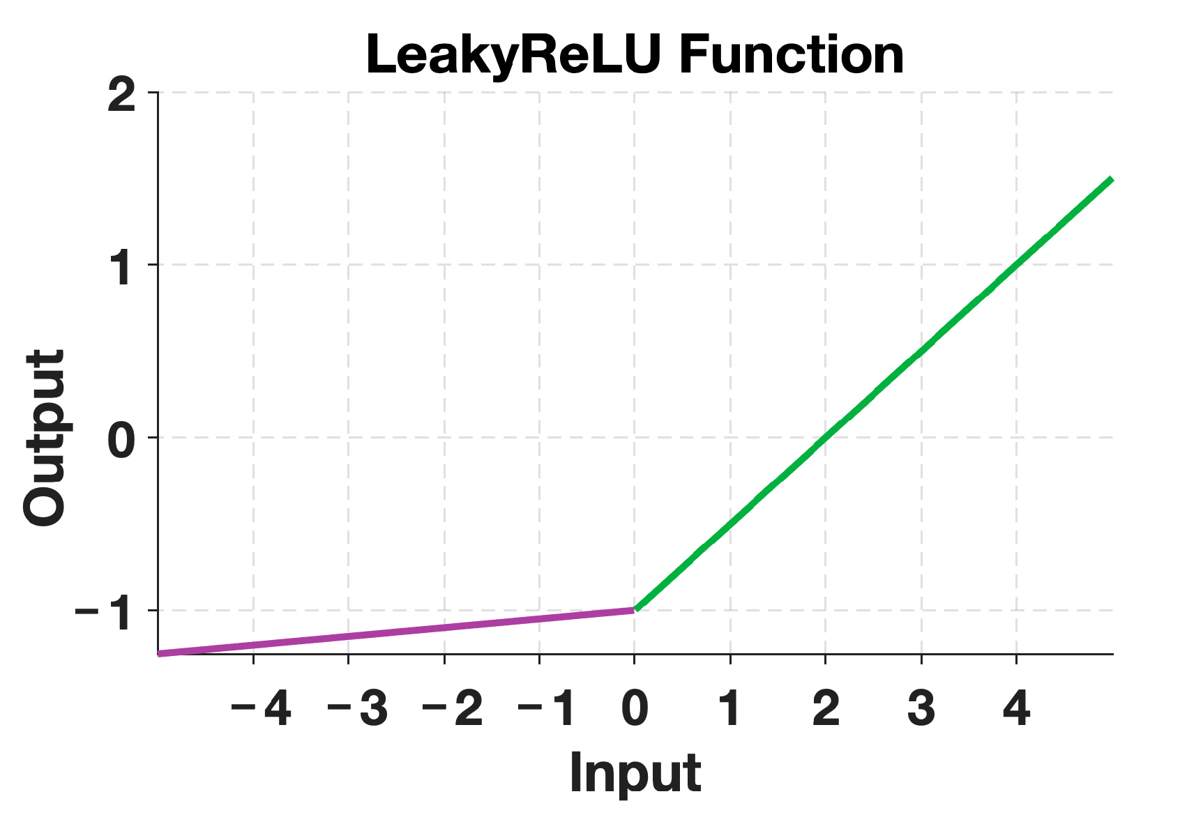
In this paper, we utilize the SE-ResNet18 architecture, which incorporates the SE module into ResNet18. Additionally, we replace the ReLU activation function with the LeakyReLU [22] activation function to improve the model’s robustness and generalization. Equation (16) shows the expression for the LeakyReLU activation function:
Figure 11 displays the image of the LeakyReLU activation function with a value of = 0.01. The purple part represents the output when the input is negative, while the green part represents the output when the input is positive. During the backpropagation process, the gradient can also be calculated for the negative input region of the LeakyReLU activation function. This prevents the issue of neuron “death” and jaggedness in the gradient direction.
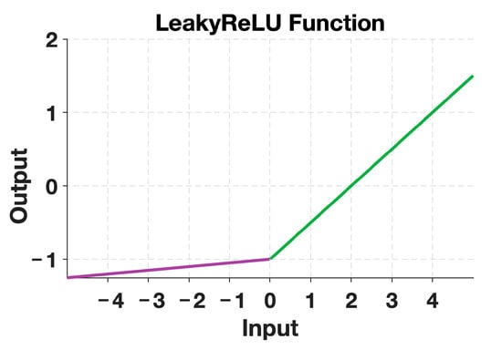
Figure 11.
LeakyReLU activation function.
3.3.3. Model Structure
The improved residual module in SE-ResNet18 has been entirely constructed. Figure 12 illustrates the structure of the improved residual module after integrating the SE module:
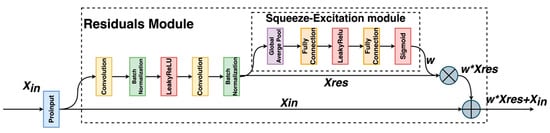
Figure 12.
Improved residual module structure.
The improved residual module takes the output of the previous network layer as input and processes it through the residual module, generating the output . is then fed into the SE module, which calculates the weight ratios of each channel in the extracted features. The SE module outputs the channel weights , which are multiplied by on a per-channel basis, added to the original input , and used to obtain the new residual term .
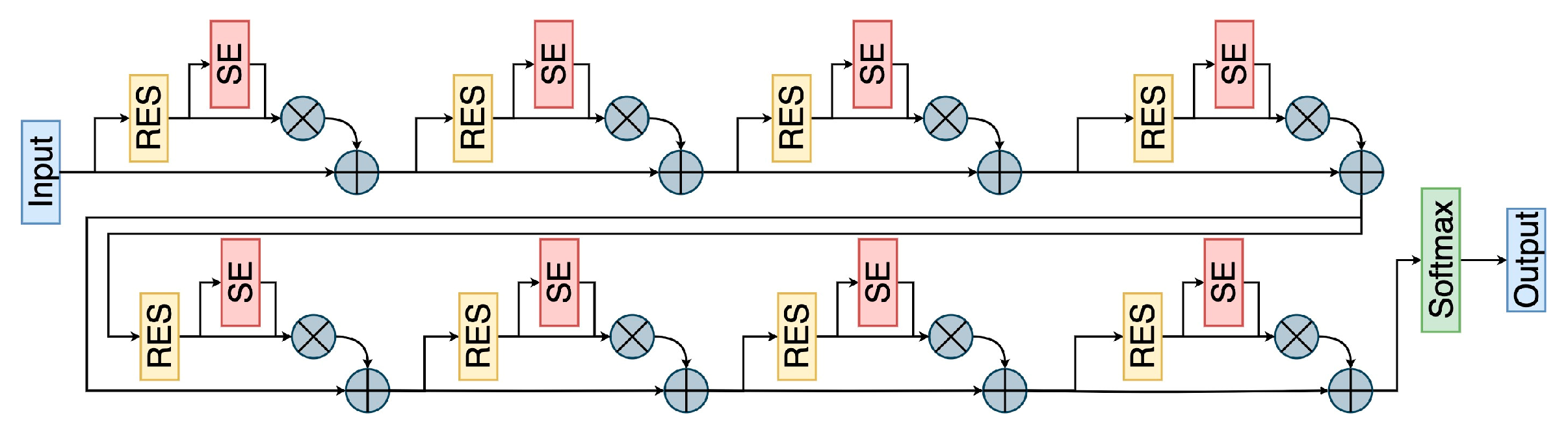
Figure 13 presents the structure diagram of the SE-ResNet18 network, where the blue part denotes the input and output of the model, the yellow part represents the residual module, the red part depicts the SE module, the green part denotes the classification function, and the gray part represents the corresponding operators.
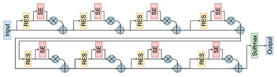
Figure 13.
SE-ResNet18 network structure.
4. Experimental Verifications
4.1. Sample Enhancement Experiment
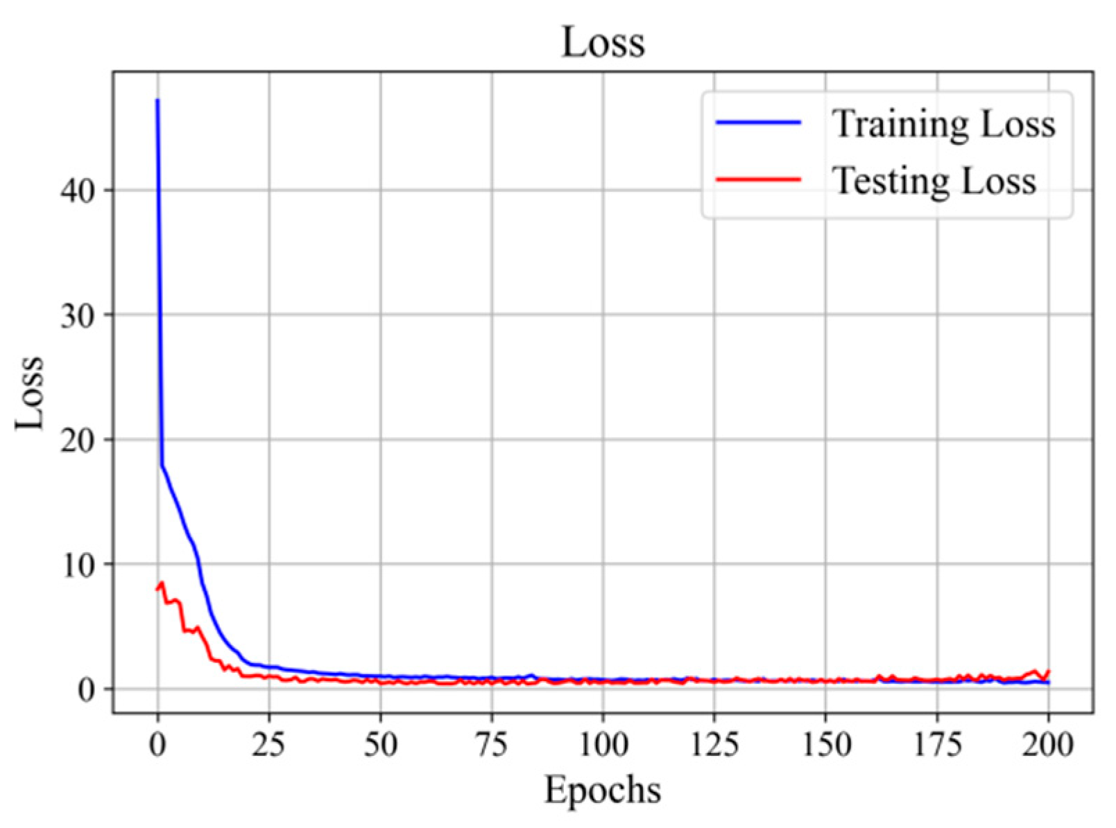
This paper proposes using a conditional variational autoencoder (CVAE) to augment a limited number of original fault samples. The dataset comprises 550 samples, divided into 21 fault categories and a normal category, each containing 25 sample files. For model training and validation, we divide these data into a training set and a test set. The CVAE model takes the original acquisition sample data as input and uses a loss function composed of KL divergence loss and reconstruction loss. The CVAE model is trained until the loss converges, and then an equal number of enhanced samples as the original samples are generated from the saved model. Figure 14 shows the training and testing loss curves for the CVAE model.
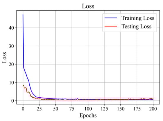
Figure 14.
CVAE model training and testing loss change curves.
Figure 14 illustrates the changing relationship between the number of training rounds and the training loss. It can be observed that the model starts training with a high loss, but the loss rapidly converges as the training progresses. After a few iterations, the model reaches a stable state, and the loss on the test set can be aligned with the loss on the training set. With faster model convergence and lower losses, the model can generate samples that closely resemble real ones. The CVAE generates twice as much data as the original dataset.
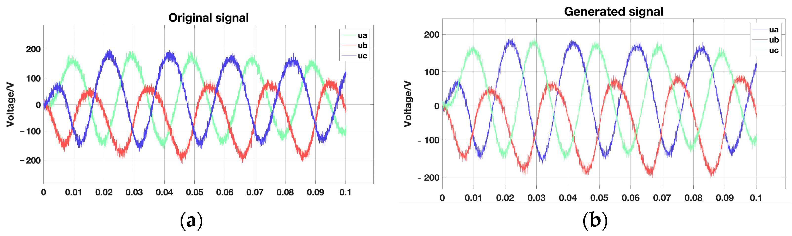
Figure 15 shows the results of comparing the original signal with the visualization of the generated signal. Upon examining the evolution of the signals, it becomes apparent that the CVAE model generates a synthetic signal that bears a strong resemblance to the original one. This is achieved by learning and comprehending the inherent structure and distribution of the input data. The original data are processed using the CVAE model, which generates new samples. These samples demonstrate a strong level of coherence with the original data, maintaining similar statistical properties and distributions across all significant features. This suggests that the CVAE model effectively captures the essential attributes of the original data and utilizes these characteristics to generate new data samples.
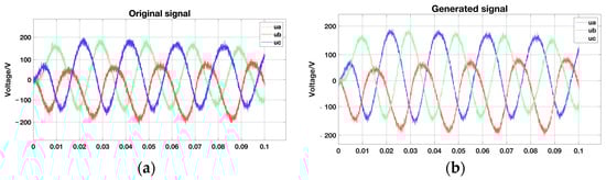
Figure 15.
Original signal and Generate signal. (a) Original signal; (b) Generated signal.
4.2. Improved Deep Residual Network Fault Diagnosis Experiment
The SE-ResNet18 model proposed in this paper is compared with the BPNN and LeNet18 model from the other research and the original ResNet18 model. The model parameters are set as follows. The structure of the BPNN, CNN, and ResNet18 models is shown in Table 2, and the parameters for ResBlock and SEResBlock are given in Table 3:
Table 2.
Parameter settings for each model.
Table 3.
Parameter details of ResBlock and SEResBlock.
The SE-ResNet18 models were trained using the Adam optimizer with a learning rate of 1 × 10⁻³ and a maximum of 50 training epochs. The test accuracy of the models is compared as follows.
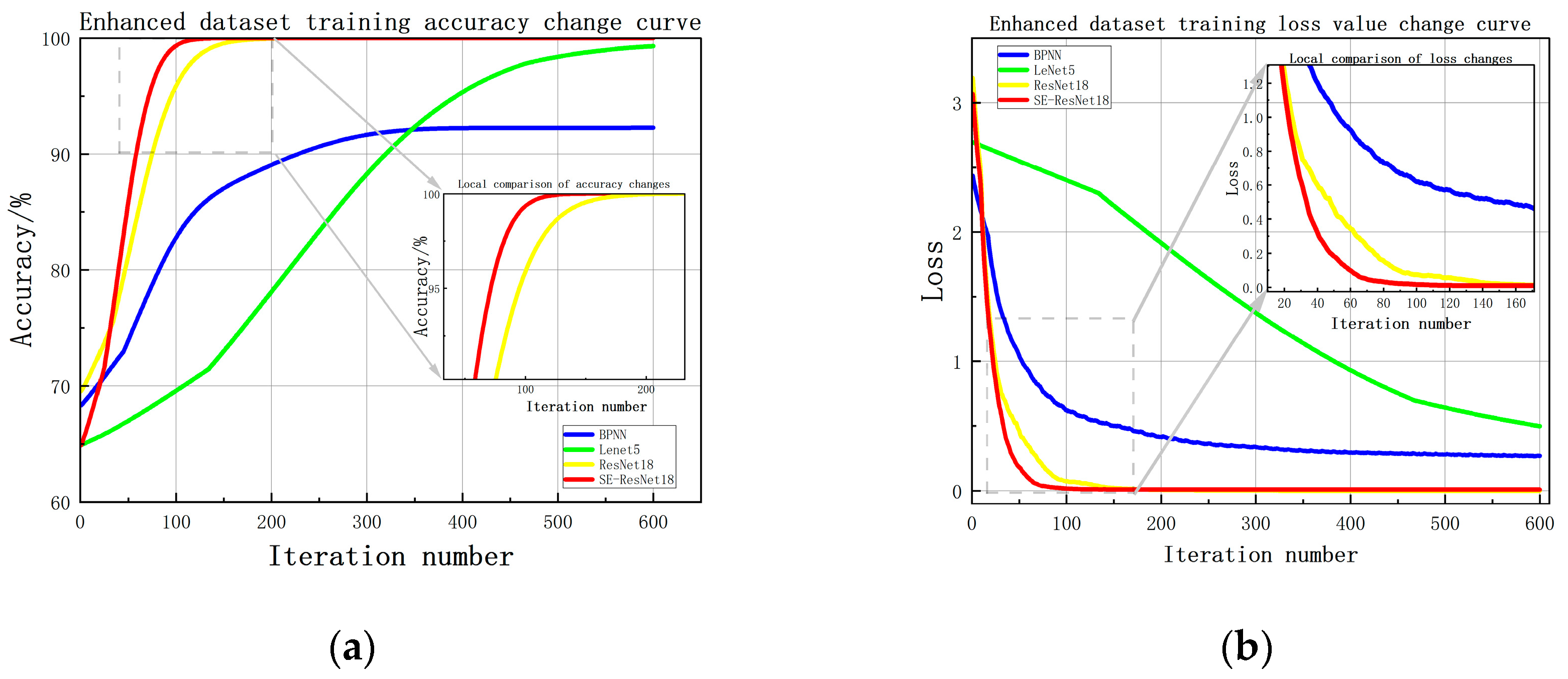
Figure 16 shows the curves depicting the variation of training accuracy and loss in the enhanced dataset. It can be observed that the improved residual neural network used as the fault diagnosis model outperforms the simple BP neural network and simple CNN network in terms of training accuracy and convergence speed. The BP neural network performs poorly, while the CNN network converges slowly as the number of samples increases, indicating a need for better optimization. Comparing ResNet18 with SE-ResNet18, where red represents the SE-ResNet18 model and yellow represents the ResNet18 model, the former achieves higher accuracy more quickly due to the addition of the SE module and the replacement of the activation function. The model also converges more quickly and produces superior results.
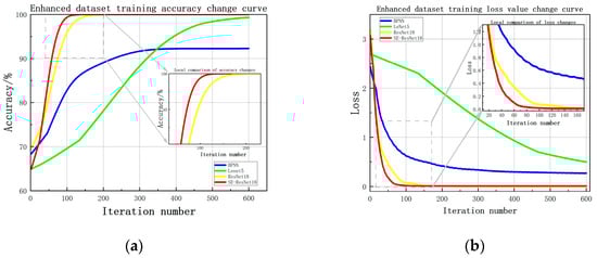
Figure 16.
Training accuracy and loss variation curves using augmented dataset. (a) Accuracy variation curve; (b) Loss variation curve.
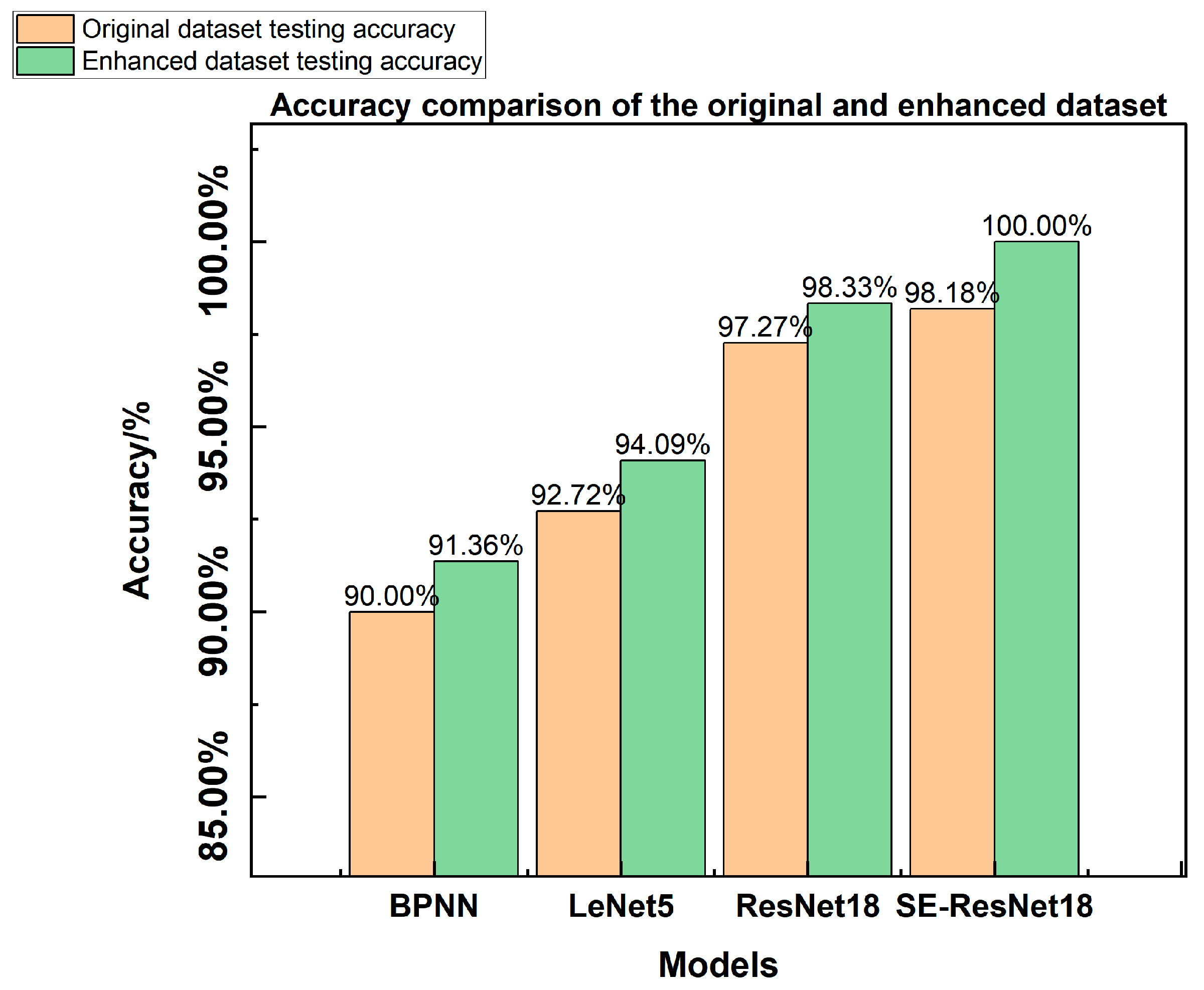
Table 4 and Figure 17 illustrate a comparison of the accuracy of diagnostic test sets for different types of fault diagnosis models.
Table 4.
Test set accuracy for each type of fault diagnosis model.
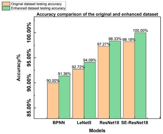
Figure 17.
Accuracy comparison of the original and enhanced datasets.
This paper divides the original dataset into training and test sets in a ratio of 7:3 for testing and training the model. This means that the 550 fault samples mentioned earlier are divided proportionally. The original dataset is denoised, and additional samples are generated to create an augmented dataset. The total number of samples is now 2200, with 1100 containing noise and 1100 denoised. The dataset is then divided in a 7:3 ratio, resulting in 1540 samples in the training set and 660 samples in the test set.
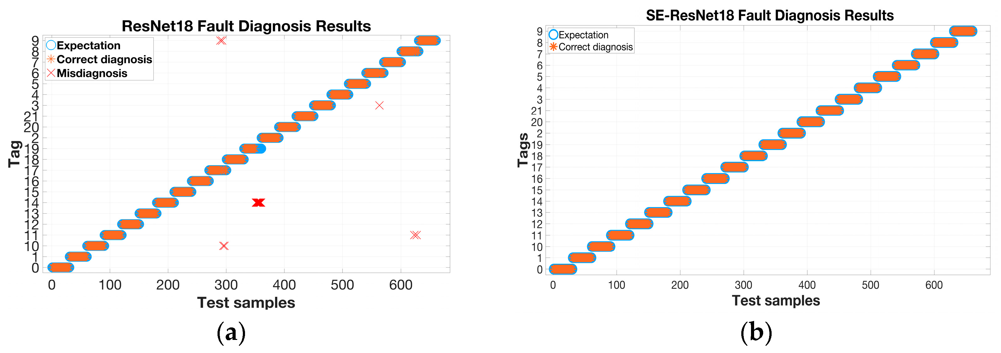
The experimental results in Table 4 and Figure 17 demonstrate that data augmentation improves the diagnostic accuracy of fault diagnosis models by extracting additional features from fault samples. Simple models, such as the BP neural network, achieve a maximum accuracy of 92% on both the original and augmented datasets. Diagnostic accuracy can be improved by utilizing convolutional neural networks, although the basic LeNet5 model still requires further enhancement. Compared with ResNet18, the SE-ResNet18 model with the added SE module achieves higher accuracy in both the original and augmented datasets. Furthermore, it maintains 100% accuracy even with the increased number of samples, demonstrating the superior performance of the SE-ResNet18 model for inverter fault diagnosis. Figure 18a,b show the results of the fault diagnosis. The plot on the left shows cases of misdiagnosis when using the ResNet18 network for fault diagnosis. In these cases, 4# and 5# faults are incorrectly diagnosed as 2# and 4# faults and 2# and 5# faults, respectively. In the figure, ‘×’ is used to represent it. In contrast, the right plot indicates that all test samples are correctly diagnosed when using SE-ResNet18 for fault diagnosis. This further demonstrates the high accuracy of the proposed model for inverter fault diagnosis.

Figure 18.
Misdiagnosis and correct diagnosis situations. (a) ResNet18 fault diagnosis results; (b) SE-ResNet18 fault diagnosis results.
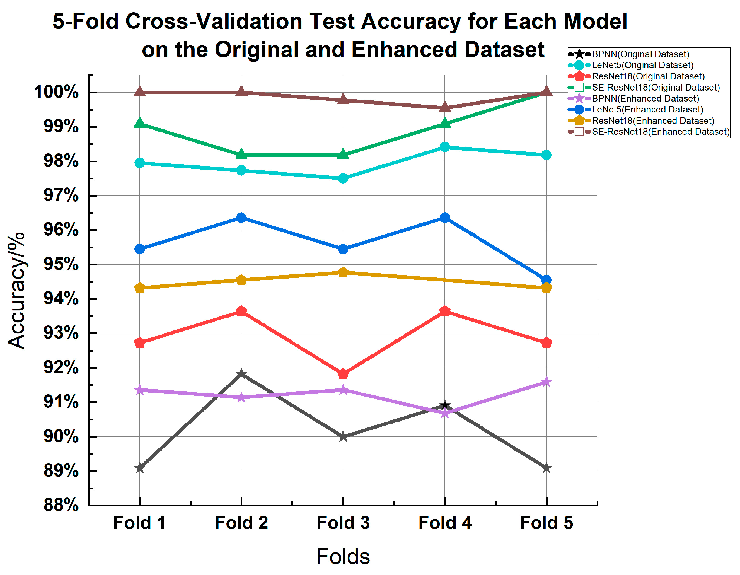
To validate the effectiveness of our proposed model, we conducted a 5-fold cross-validation on both the original and augmented datasets. Table 5 and Table 6 outline the details of these cross-validation results. A notable observation from Figure 19 is the consistently high accuracy achieved by our proposed method across multiple experiments. This consistently high performance not only demonstrates the strength of our model but also emphasizes its validity.
Table 5.
Five-fold cross-validation test accuracy for each model on the original dataset.
Table 6.
Five-fold cross-validation test accuracy for each model on the enhanced dataset.
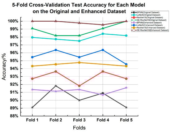
Figure 19.
Five-fold cross-validation test accuracy for each model on the original and enhanced dataset.
5. Conclusions
This study employs a CVAE for data augmentation of fault samples and a WPD denoising method to eliminate noise from the samples. This approach aims to enhance the performance of the fault diagnosis model. A fault diagnosis model called SE-ResNet18, based on the channel attention mechanism, is proposed. The experimental results demonstrate that the augmented dataset improves the fault diagnosis of three-phase inverters. Moreover, SE-ResNet18 achieves high diagnostic accuracy in fault diagnosis, faster convergence speed, and shorter iteration epochs than other models.
This study has several significant contributions and advantages. Firstly, the issue of a limited number of samples is addressed by utilizing CVAE to augment the original samples. This approach extends the dataset and explores the potential features of the fault samples, enhancing the prominence of the sample features and improving the accuracy of fault diagnosis. Furthermore, the sample normalization method is used to convert the faulty samples into grayscale maps. This approach offers a new way of processing inverter samples, making the model more generalizable and improving iteration speed. Lastly, by introducing the channel attention mechanism, the attention to the weight relationship between channels is enhanced, thereby further improving the model’s accuracy and performance of the model.
To summarize, the proposed method for deep residual network fault diagnosis, which incorporates data augmentation and the channel attention mechanism, demonstrates high accuracy and performance in practical applications. This method provides an effective solution for diagnosing inverter faults. Future research can focus on exploring additional advanced data enhancement techniques and network structures to further enhance the generalization capability and practicality of the fault diagnosis model.
6. Discussion
Our study has made significant progress in the fault diagnosis of three-phase inverters, utilizing techniques such as WPD, CVAE, and SE-ResNet18. Despite this progress, there are several areas that require further exploration and improvement.
Primarily, the effectiveness of our approach heavily relies on the availability of high-quality initial fault samples. Our method to augment both the quantity and quality of samples depends on these initial samples. Any existing bias or errors in these initial samples could potentially compromise the accuracy of the final fault diagnosis.
Secondly, applying wavelet packet denoising (WPD) introduces the challenge of selecting an appropriate wavelet packet base function. This decision isn’t always straightforward and may require extensive experimentation and adjustment.
Furthermore, the utilization of CVAE for sample enhancement involves adjusting numerous hyperparameters. The selection of these parameters can significantly influence the quality of the enhanced samples and the overall effectiveness of the fault diagnosis. In future research, the adoption of swarm intelligence optimization algorithms, such as the Dung Beetle Optimizer (DBO) [23] or the Sparrow Search Algorithm (SSA) [24], might prove beneficial. These algorithms can optimize the hyperparameters of the model, resulting in an optimal combination that improves performance.
Therefore, future endeavors should further investigate these issues to enhance our fault diagnosis methodology, with the goal of improving its accuracy and expanding its scope.
Author Contributions
Conceptualization, Y.F.; formal analysis, Y.F. and X.B.; funding acquisition, Y.F. and G.M.; investigation, Y.J. and X.B.; methodology, Y.J.; resources, Y.F., G.M., W.C. and X.B.; software, Y.J.; supervision, Y.F., X.B., G.M., and W.C.; validation, Y.J., X.B.; writing—original draft, Y.J. and Y.F.; writing—review and editing, Y.J., Y.F., and X.B. All authors have read and agreed to the published version of the manuscript.
Funding
This research received no external funding.
Data Availability Statement
Not applicable.
Conflicts of Interest
The authors declare no conflict of interest.
References
- Cao, R.J.; Guo, Q.Y. Fault Diagnosis Technique for Three-level Inverters Based on ICEEMDAN-FE and Support Vector Machine. Locomot. Electr. Drive 2023, 1, 97–103. [Google Scholar]
- Chen, T. Research on Open-Circuit Fault Diagnosis Method for Three-Phase Voltage Source Inverters. Ph.D. Thesis, University of Science and Technology Beijing, Beijing, China, 2021. [Google Scholar] [CrossRef]
- Song, W.; Shi, W.F.; Zhuo, J.B.; Xie, J.L. A Review of Fault Diagnosis Methods for Multilevel Inverters. Micromotors 2019, 52, 110–117. [Google Scholar]
- Xu, S.Q.; Huang, W.Z.; He, Y.G.; Hu, Y.Q.; Cheng, T.L. Diagnosing Open-Circuit Faults in Three-Level Grid-Connected Inverters Based on an Adaptive Sliding-Mode Observer. Trans. China Electrotech. Soc. 2023, 38, 1010–1022. [Google Scholar]
- Fan, P.S.; Pazilai, M.H.M.; Wei, S.F.; Liu, S. Early Fault Parameter Identification for Grid-Connected Inverters Based on a Model. J. China Three Gorges Univ. (Nat. Sci.) 2022, 44, 64–69. [Google Scholar]
- Li, X.; Li, S.; Chen, W.; Shi, T.; Xia, C. A Fast Diagnosis Strategy for Inverter Open-Circuit Faults Based on the Current Path of Brushless DC Motors. IEEE Trans. Power Electron. 2023, 38, 9311–9316. [Google Scholar] [CrossRef]
- Shen, H.L.; Tang, X.; Luo, Y.F.; Xiao, F.; Ai, S.; Fan, Y.S. Diagnosis of Open-Circuit Faults in Three-Phase Inverters Based on CNN and Analysis of Sample Conditions. J. Natl. Univ. Defense Technol. 2022, 44, 163–172. [Google Scholar]
- Yu, H.; Deng, J.J.; Wang, Z.P.; Sun, F.C. Inverter Fault Diagnosis Method Based on Convolutional Neural Network. Automot. Eng. 2022, 44, 142–151. [Google Scholar]
- Xu, X.J.; Yu, F. Fault Diagnosis of Open-Circuit Switches in Three-Phase Inverters Based on Output Voltage Trajectory. Proc. CSEE 2023, 43, 1–11. [Google Scholar]
- Zhu, Q.Y.; Li, Y.L.; Tan, X.T.; Wei, W.; Li, A.H. Extraction of IGBT Minor Fault Features Based on Multimodal Output Voltage of Inverter. Electr. Mach. Control 2023, 27, 65–79. [Google Scholar]
- Sun, X.; Song, C.; Zhang, Y.; Sha, X.; Diao, N. An Open-Circuit Fault Diagnosis Algorithm Based on Signal Normalization Preprocessing for Motor Drive Inverter. IEEE Trans. Instrum. Meas. 2023, 72, 3513712. [Google Scholar] [CrossRef]
- Yang, H.; Peng, Z.; Xu, Q.; Huang, T.; Zhu, X. Inverter Fault Diagnosis Based on Fourier Transform and Evolutionary Neural Network. Front. Energy Res. 2023, 10, 1090209. [Google Scholar] [CrossRef]
- Yan, H.; Peng, Y.; Shang, W.; Kong, D. Open-Circuit Fault Diagnosis in Voltage Source Inverter for Motor Drive by Using Deep Neural Network. Eng. Appl. Artif. Intell. 2023, 120, 105866. [Google Scholar] [CrossRef]
- Sun, Q.; Peng, F.; Li, H.S.; Yu, X.H.; Sun, G.D. Inverter Fault Diagnosis Method Based on CGAN-CNN under Imbalanced Samples. J. Chin. Soc. Power Eng. 2022, 42, 1–14. [Google Scholar]
- Cui, Y.; Wang, R.; Si, Y.; Zhang, S.; Wang, Y.; Lin, A. T-Type Inverter Fault Diagnosis Based on GASF and Improved AlexNet. Energy Rep. 2023, 9, 2718–2731. [Google Scholar] [CrossRef]
- Łuczak, D.; Brock, S.; Siembab, K. Fault Detection and Localization of a Three-Phase Inverter with Permanent Magnet Synchronous Motor Load Using a Convolutional Neural Network. Actuators 2023, 12, 125. [Google Scholar] [CrossRef]
- Li, Z.; Liu, F.; Yang, W.; Peng, S.; Zhou, J. A Survey of Convolutional Neural Networks: Analysis, Applications, and Prospects. IEEE Trans. Neural Netw. Learn. Syst. 2021, 33, 6999–7019. [Google Scholar] [CrossRef]
- He, K.; Zhang, X.; Ren, S.; Sun, J. Deep Residual Learning for Image Recognition. In Proceedings of the IEEE Conference on Computer Vision and Pattern Recognition, Las Vegas, NV, USA, 27 June 2016; pp. 770–778. [Google Scholar]
- Kingma, D.P.; Welling, M. Auto-Encoding Variational Bayes. arXiv 2013, arXiv:1312.6114. [Google Scholar]
- Gao, R.X.; Yan, R. Wavelet Packet Transform. In Wavelets: Theory and Applications for Manufacturing; Springer: Berlin/Heidelberg, Germany, 2011; pp. 69–81. [Google Scholar]
- Hu, J.; Shen, L.; Sun, G. Squeeze-and-Excitation Networks. In Proceedings of the IEEE Conference on Computer Vision and Pattern Recognition, Salt Lake City, UT, USA, 18 June 2018; pp. 7132–7141. [Google Scholar]
- Maas, A.L.; Hannun, A.Y.; Ng, A.Y. Rectifier Nonlinearities Improve Neural Network Acoustic Models. Proc. ICML 2013, 30, 1–3. [Google Scholar]
- Xue, J.; Shen, B. Dung Beetle Optimizer: A New Meta-heuristic Algorithm for Global Optimization. J. Supercomput. 2023, 79, 7305–7336. [Google Scholar] [CrossRef]
- Xue, J.; Shen, B. A Novel Swarm Intelligence Optimization Approach: Sparrow Search Algorithm. Syst. Sci. Control. Eng. 2020, 8, 22–34. [Google Scholar] [CrossRef]


Disclaimer/Publisher’s Note: The statements, opinions and data contained in all publications are solely those of the individual author(s) and contributor(s) and not of MDPI and/or the editor(s). MDPI and/or the editor(s) disclaim responsibility for any injury to people or property resulting from any ideas, methods, instructions or products referred to in the content. |
© 2023 by the authors. Licensee MDPI, Basel, Switzerland. This article is an open access article distributed under the terms and conditions of the Creative Commons Attribution (CC BY) license (https://creativecommons.org/licenses/by/4.0/).