Cost-Efficient Two-Level Modeling of Microwave Passives Using Feature-Based Surrogates and Domain Confinement

Abstract

A variety of surrogate modeling techniques has been utilized in high-frequency design over the last two decades. Yet, the curse of dimensionality still poses a serious challenge in setting up reliable design-ready surrogates of modern microwave components. The difficulty of the modeling task is only aggravated by nonlinearity of circuit responses. Consequently, constructing a practically usable surrogate model, valid across extended ranges of material, geometry, and operational parameters, is far from easy. As a matter of fact, conventional modeling techniques are merely capable of building models for microwave structures featuring a relatively small number of designable parameters within reduced ranges thereof. One possible way of mitigating these obstacles may be the employment of the recently proposed two-stage performance-driven modeling approach. Therein, the surrogate model domain is narrowed down to the section of the space where the vectors of adequate quality are located, thereby permitting significantly reducing the cost of acquiring the training data. Seeking even further cost reduction, this work introduces a novel modeling framework, which exploits problem-specific knowledge extracted from the circuit responses to achieve substantial cost-savings of training data acquisition. In our methodology, the modeling procedure targets response features instead of the complete responses. The response features are the characteristic locations of the circuit response, such as relevant minima or maxima over selected frequency bands. The dependency of the coordinates of the said features on circuit dimensions is considerably less nonlinear than is observed for the complete characteristics, which enables sizable reduction of the data acquisition cost. Numerical validation of our procedure involving three microwave structures corroborates its remarkable efficiency, which allows for setting design-ready surrogates using only a handful of samples.

1. Introduction

The use of full-wave electromagnetic (EM) simulation software is a standard practice in microwave design today. EM analysis is being used throughout the entire design cycle of microwave devices and systems, starting from topology development [1,2,3,4] through parametric studies [5], to the final refinement of circuit dimensions [6,7,8,9,10,11]. This is primarily because EM analysis is able to accurately account for various phenomena exerting significant effects on circuit responses, such as EM cross-coupling [12,13,14,15,16,17]. Furthermore, the incorporation of size reduction techniques of various kinds (e.g., use of the slow-wave phenomenon [18,19,20,21], transmission line folding [22,23], defected ground structures [24,25], or multi-layer realizations [26,27,28]) makes the topologies of microwave devices increasingly intricate. Another important factor affecting their geometries is the implementation of additional functionalities, e.g., wide-band [29,30,31] or multi-band operation [32,33,34] or harmonic attenuation [35,36,37]. Devices featuring complex geometries have to be evaluated using EM analysis, which is accurate yet tends to be computationally expensive. Consequently, the designers face a situation in which they are in possession of powerful simulation tools, yet the cost of their repetitive usage within simulation-based design procedures might be impractical. In particular, multitudinous simulations, indispensable when solving such tasks as local optimization [38,39,40], global search [41,42,43], or multi-objective optimization [44,45,46,47], may last far too long.

Not surprisingly, alternative ways of rendering accurate responses of microwave components have been sought. A popular approach is to replace costly EM simulations with surrogate models. Numerous surrogate modeling techniques have been devised and applied in microwave design. There exist two primary categories of surrogates: data-driven and physics-based models. The former come in many variations (e.g., kriging [48,49,50], neural networks [51,52,53,54,55], radial basis functions [56,57], and Gaussian process regression [58,59] to name just a few). They are exploited by global search procedures [60] and multi-criterial optimization [61] and frequently combined with sequential sampling routines [62,63]. Their advantages are simplicity of implementation, flexibility, and abundance of the available techniques [64,65,66,67]. Disadvantages are associated with the curse of dimensionality having a strong adverse effect on the modeling process in terms of the number of designable variables that may be taken into consideration, as well as their ranges.

The surrogates of the second class, i.e., physics-based ones, make use of the problem-relevant knowledge encoded as an auxiliary low-fidelity model (e.g., an equivalent circuit [68,69]). As a consequence, physics-based models feature enhanced generalization capability [70]. The most popular modeling technique utilizing physics-based surrogates is arguably space mapping (SM) [71,72,73,74,75,76] along with its numerous variations such as aggressive [77], implicit [78], or frequency SM [79]. Still, the necessity to devise a problem-dependent low-fidelity model significantly narrows down the application areas in which physics-based models may be utilized.

A remedy for the aforementioned problems is the employment of the recently developed performance-driven modeling techniques [80,81,82]. Therein, the surrogate model domain is constricted to the section of the design space enclosing superior-quality designs according to the assumed performance specifications. In contrast to the conventional domain, typically delineated by the lower and upper limits of circuit dimensions, the volume of the domain constrained in line with the performance-driven modeling concept is dramatically smaller. This begets a considerably lower cost of training data collection. Yet, the cost-effectiveness of triangulation-driven confined modeling [80] and the nested kriging modeling technique [81], the initial versions of performance-driven modeling techniques, has been seriously limited by the fact that surrogate model domain is identified with the use of database designs. The said designs (also referred to as reference points) have to be optimized beforehand according to the pre-selected values of the design specifications, incurring hefty computational cost. Several attempts to improve the efficacy of the nested kriging modeling technique have been made starting from enhanced sampling [83], through variable-fidelity setup [84], dimensionality reduction [85], and adopting variable-thickness domain [86], up to gradient-enhanced nested kriging [87]. In the latter, sensitivity data derived from the reference designs have been exploited, which made it possible to cut down the number of the database designs by half.

A more recent development, i.e., no-reference-design (or observable based) constrained modeling [82], allowed for a substantial reduction of these expenditures by delimiting the confined domain based on a collection of pre-selected random observables, a gathering of which did not involve any optimization problems whatsoever. In [82], the process of accepting and rejecting the observables exploits the knowledge gathered from the observables themselves allowing for a cost-efficient surrogate domain definition. Recently, several advancements of the technique of [82] have been reported that aimed at improving the surrogate accuracy or decreasing the training data acquisition cost. These include dimensionality reduction using principal component analysis [88], modeling the responses of microwave components using neural networks [89] (instead of kriging interpolation as in [82]), or incorporation of variable-fidelity models [90]. Still, in all the aforementioned techniques, the modeling process has been carried out on the entire component’s characteristics.

To push the efficacy of the modeling process further, this work introduces a novel technique, which integrates the no-reference-design confined modeling methodology with the response feature technology [91]. In our approach, the confined domain of the surrogate model is assessed cost-efficiently as in [82], yet, instead of constructing the surrogate that renders the entire frequency characteristics of a microwave component at hand, here, the modeling process is carried out solely at the level of the response features. The coordinates of the features depend weakly and nonlinearly on the structure geometry parameters. Exploiting the problem-specific knowledge embedded in the circuit responses allows for achieving an additional reduction of the expenses associated with acquiring training data that may be obtained versus that of the modeling routine processing the complete responses, without degrading the modeling accuracy. Another advantage of our approach is that it allows for handling wide ranges of both circuit dimensions and material/operating parameters spread over the constructed surrogates. The comprehensive validation of the introduced procedure includes benchmarking against five conventional modeling techniques (kriging [48], radial basis functions [56], artificial neural networks [51], convolutional neural networks [92], and ensemble learning [93]), as well as two constrained modeling techniques: nested kriging [81] and no-reference-design constrained modeling [82]. The verification structures include three microstrip circuits. The outcome of the conducted experiments corroborates the remarkable efficiency of our procedure: reliable surrogates have been rendered at an average cost of merely one hundred training data samples. The technical contributions and the originality of the work include (i) the introduction of the response feature technology into the recent observable-based performance-driven modeling technique; (ii) implementation of a complete framework for modeling of passive microwave components, which capitalizes on the mentioned algorithmic tools; (iii) demonstrating the ability of constructing reliable behavioral models across a wide range of geometric variables and operational conditions with a small number of training points; and (iv) demonstrating enhanced performance of the developed technique with respect to the predictive power of the constructed surrogates and computational efficiency over a wide selection of state-of-the-art benchmark techniques. More importantly, the presented approach demonstrated a possibility of predicting the operating parameters of the microwave circuits in an extremely reliable manner (a fraction of a percent for the operating frequencies, and a small fraction of dB for power split ratios) using datasets containing a few dozens of samples, which is far beyond the capability of any other technique available in the literature.

2. Two-Stage Feature-Based Modeling

This section outlines the developed modeling framework, in which the surrogate model domain confinement conforms with the performance-driven modeling paradigm [82], and the modeling process itself targets the response features [91]. Section 2.1 recalls the concepts of the domain confinement based on the pre-selected observables. The basics of the response feature technology and employing the problem-specific knowledge to enhance the efficacy of the developed modeling procedure are delineated in Section 2.2, which also provides the description of the proposed modeling routine.

2.1. Two-Stage Performance-Driven Modeling

Constrained modeling methods [80,81,82] share the same underlying concept of restraining the modeling process to the encouraging segment of the design space, where the designer expects that designs satisfying the assumed specs likely reside. The paramount difference between the techniques [80,81,82] consists in the way the location of this section of the design space is assessed. Both the triangulation-based modeling technique [80] and the nested kriging modeling technique [81] require a database of pre-optimized parameter vectors for delimiting the surrogate domain. Clearly, this may call the efficiency of the entire modeling process into question, as the associated computational expenditures might be equal to several hundred or even thousands of EM analyses of the component of interest. As mentioned in Section 1, the development of the no-reference-design modeling technique [82] rendered the cost of setting up a constrained modeling framework practically acceptable. The basic concepts behind this approach are briefly outlined in this section.

Table 1. Basic notation used by performance-driven modeling methods.

Description	Notation
Vector of geometry parameters	x = [x1 … xn]T
Conventional design space	X = [l, u]
Lower bounds on parameters	l = [l1 …, ln]T
Upper bounds on parameters	u = [u1 …, un]T
Performance figures	fk, k = 1, …, N
Space of design objectives	F: fk.min ≤ fk(j) ≤ fk.max, k = 1, …, N
Vector of objectives	F = [f1 … fN]T

presents the notation shared by performance-driven modeling techniques. There exist two spaces: the design space X, along with the space of design objectives F. The components of vector F represent the design objectives such as intended operating frequency (or frequency band) of a microwave component of interest, target power division, or permittivity of a substrate the device is realized on. The ranges of design objectives delimit the intended surrogate’s region of validity.

In this work, the model domain is defined according to the procedure proposed in [82]. Let us denote as {x_r^(j), f_r^(j)}, j = 1, 2, …, a set of pairs: observables x_r^(j) allocated in the design space X according to uniform probability distribution, along with the associated objective vectors F_r^(j) (extracted from the responses at x_r^(j)). The observables undergo a selection procedure (until the assumed number of observables N_r is acquired): points whose performance figure vector F_r^(j) belongs to F are accepted, and others are discarded. In practice, N_r should be set at around 10n (n being the parameter space cardinality). The accepted pairs {x_r^(j), F_r^(j)}, j = 1, …, N_r, form a training set for building the inverse surrogate s_r, which plays a crucial role in the domain definition process. (The details can be found in [82]).

Ultimately, the forward surrogate s(x) is put together within the domain X_S as a kriging interpolation surrogate [86]. The training dataset for constructing s(x) includes the pairs {x_B^(k), R_B^(k)}_{k = 1, …, NB}, where x_B^(k) ∈ X_S are the data points, and R_B are the corresponding EM-evaluated circuit responses.

2.2. Two-Level Modeling Using Feature-Based Surrogates

As announced in Section 1, the proposed modeling technique operates on the appropriately selected characteristic points of circuit characteristics, instead of the entire responses. This permits smoothening of the functional dependencies to be represented by the surrogates, as the dependency of the characteristic points on the component dimensions is to a lesser extent nonlinear compared to a similar dependence for complete frequency characteristics of microwave components. As a consequence, due to exploiting the problem-specific knowledge, a radical reduction of the training samples’ acquisition cost may be obtained when conducting the modeling process on the layer of features. Furthermore, in the context of design optimization, response feature technology often enables quasi-global search capability while using formally local optimizers [94].

Notwithstanding, the prerequisite for employing the response feature technology is a suitable shape of the component responses with easily discernible characteristic locations (features). In practice, the response features are obtained by scanning the EM-evaluated component responses. Clearly, for some designs, certain the characteristic points are indistinguishable. This issue needs to be properly tackled during the modeling process. Moreover, from a practical standpoint, the response features are to be chosen to reflect the assumed design goals. For a detailed exposition of response feature technology see [91]. Interested readers may find an extended discussion of response feature technology along with various applications, limitations, and possible generalizations in the rich literature on the subject, e.g., [95,96].

Figure 1 shows the microwave structures employed in this work to be the verification case studies (a rat-race coupler (RRC), a branch-line coupler (BLC), and a dual-band power divider), along with their exemplary responses and characteristic points. The relevant data concerning the devices of Figure 1 are gathered in

Table 2. Essential data of verification circuits.

Parameter	Circuit Structure
	Circuit I [97]	Circuit II [98]	Circuit III [99]
Substrate	RO4003 (εr = 3.38, h = 0.76 mm)	εr—operating parameter h = 0.76 mm	AD250 (εr = 2.5, h = 0.81 mm)
Design parameters $	x = [l1 l2 l3 d w w1]T	x = [g l1r la lb w1 w2r w3r w4r wa wb]T	x = [l1 l2 l3 l4 l5 s w2]
Other parameters $	d1 = d + |w − w1|, d = 1.0, w0 = 1.7, and l0 = 15	L = 2dL + Ls, Ls = 4w1 + 4g + s + la + lb, W = 2dL + Ws, Ws = 4w1 + 4g + s + 2wa, l1 = lbl1r, w2 = waw2r, w3 = w3rwa, w4 = w4rwa	w1 = 2.2 mm, g = 1 mm
Conventional parameter space X	l = [2.0 7.0 12.5 0.2 0.7 0.2]T, u = [4.5 12.5 22.0 0.65 1.5 0.9]T	l = [0.4 0.43 5.9 7.7 0.68 0.28 0.1 0.1 2.0 0.2]T, u = [1.0 0.86 14.0 16.5 1.5 0.99 0.65 0.25 5.5 0.8]T	l = [14.5 1.1 13.0 0.5 1.6 0.19 3.9]T, u = [37.0 16.6 35.0 15.0 5.6 1.5 5.8]T
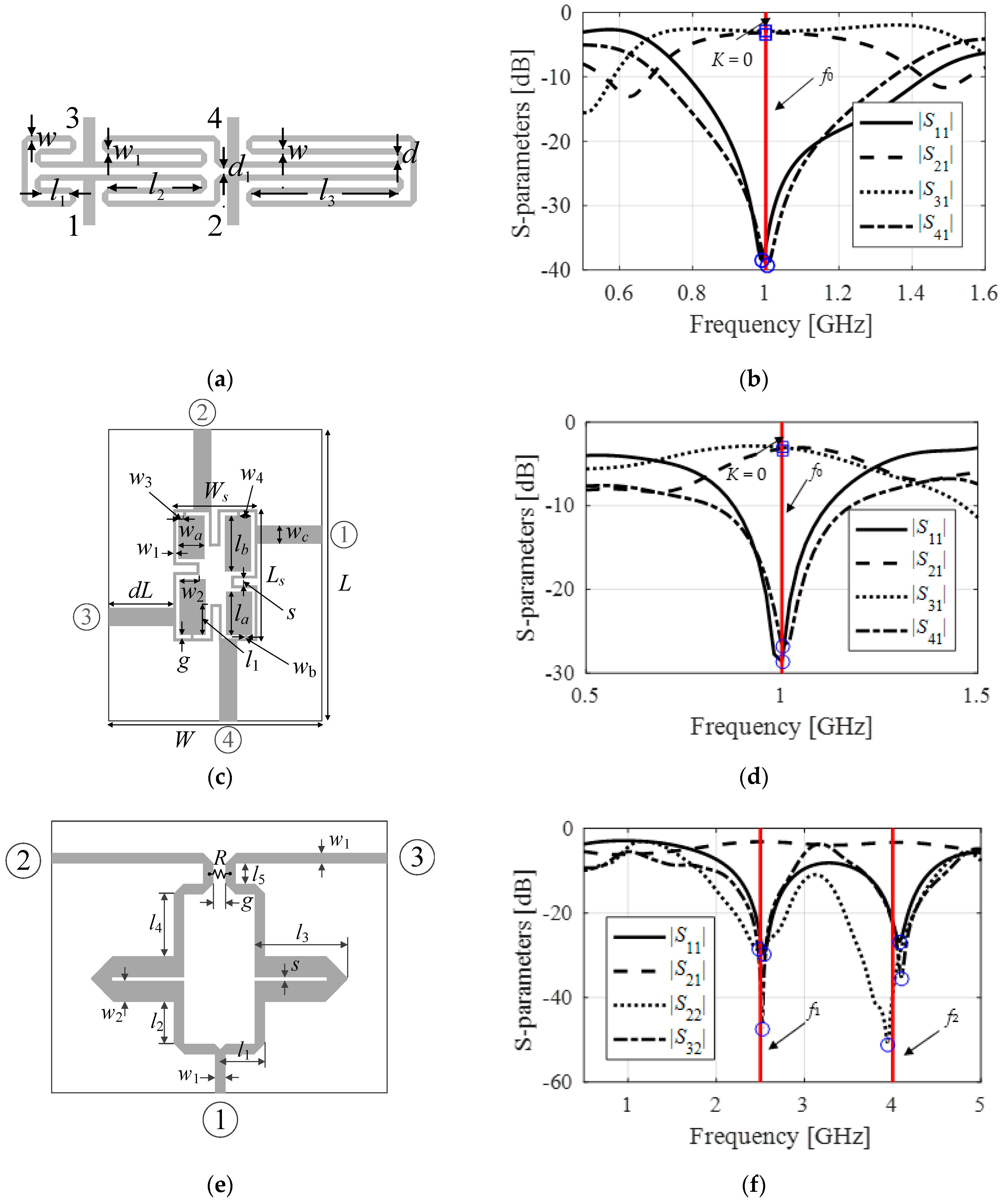
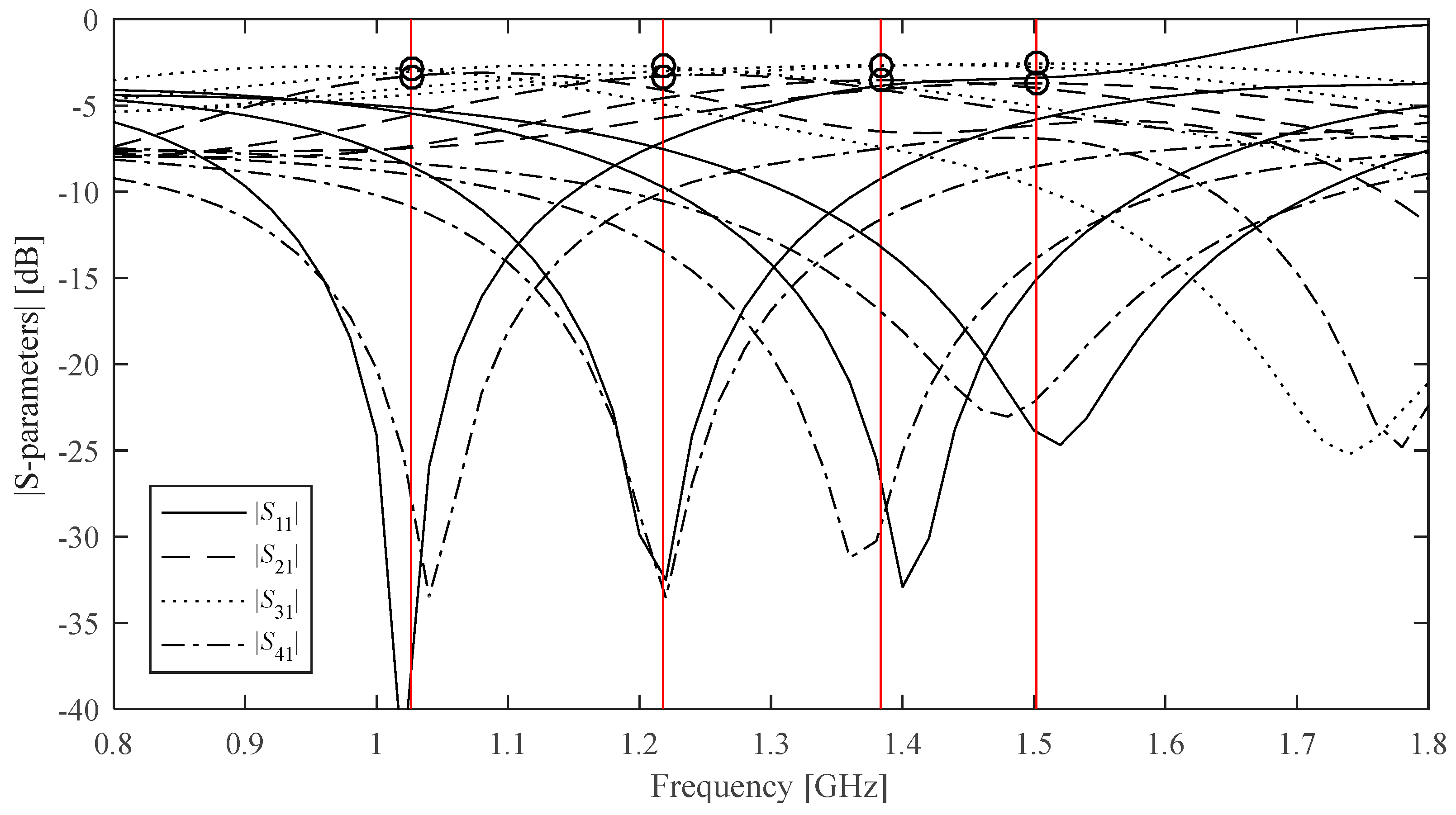
Figures of interest	Operating frequency f0 Power split ratio K	Operating frequency f0 Substrate permittivity εr	Lower band operating frequency f1 Ratio Kf = f2/f1 between upper operating frequency f2 and f1
Design objectives	Minimize matching and isolation at the target operating frequency f0 Maintain the required power split ratio K	Minimize matching and isolation at the target operating frequency f0 Maintain equal power split ratio K	Minimize matching and isolation at both target frequencies f1 and f2 Maintain equal power division ratio
Objective space	1.0 GHz ≤ f0 ≤ 2.0 GHz −6.0 dB ≤ K ≤ 0 dB	1.0 GHz ≤ f0 ≤ 2.0 GHz 2.0 ≤ εr ≤ 5.0	1.25 GHz ≤ f1 ≤ 4.0 GHz 1.4 ≤ Kf ≤ 1.8

^$ Dimensions in mm, except for those with subscript “r”, which are relative and unit-less.

, including geometry parameters, substrate, and the parameter space, as well as the figures of interest, design objectives, and the objective space. As for RRC (Circuit I) and BLC (Circuit II), the feature points are defined as the minima of the coupler’s characteristics |S₁₁| and |S₄₁|, f_min.S11 and f_min.S41, respectively. These are employed to estimate the circuit operating frequency f₀ as follows:

f₀ = (f_min.S11 + f_min.S41)/2

(1)

whereas the level coordinates l_min.S21 and l_min.S31 of the characteristic points |S₂₁(f₀)| and |S₃₁(f₀)| are utilized to assess the device’s power split at f₀ as:

K = |l_max.S21 − l_max.S31|

(2)

Thus, the aforementioned feature points suffice to handle the design objectives of Table 2, which are defined as minimization of matching and isolation at f₀, and also maintain the required value of the power split factor (equal in the case of BLC).

For a dual-band power divider (Circuit III), the sets of frequencies f_1.min.S21, f_1.min.S22, and f_1.min.S32 and f_2.min.S21, f_2.min.S22, and f_2.min.S32 corresponding to the first and the second minima, respectively, of the divider’s responses |S₂₁|, |S₂₂|, and |S₃₂| serve to estimate the circuit’s lower and upper band operating frequencies f₁ and f₂ as follows:

f₁ = (f_1.min.S21 + f_1.min.S22 + f_1.min.S32)/3

(3)

and

f₂ = (f_2.min.S21 + f_2.min.S22 + f_2.min.S32)/3

(4)

Next, the ratio between these frequencies is assessed as K_f = f₂/f_1. For the power divider, the requirement for equal power division is enforced by the symmetry of its structure. In the discussed approach, the forward surrogate s(x) is built at the response feature level (in contrast to the nested kriging [81] and no-reference-design modeling [82] techniques or the techniques proposed in [88,89,90], where complete component’s characteristics have been handled during the modeling process).

The training dataset for constructing s(x) consists of pairs {x_B^(k), F_R(x_B^(k))}_{k = 1, …, NB}, with the designs x_B^(k) randomly distributed over the confined domain X_S, whereas F_R(x_B^(k)) = [f₁(x_B^(k)) f₂(x_B^(k)) … f_p(x_B^(k)) l₁(x_B^(k)) l₂(x_B^(k)) … l_p(x_B^(k))]^T represents the feature vector for a given design x_B^(k). The vector F_R comprises the frequencies f_j and levels l_j, j = 1, …, p, of the response features of the designer’s choice. Moreover, the observables and their respective features, i.e., ({x_r^(l), F_R(x_r^(l))}_{l = 1, …, Nr}.), are also incorporated into the training set.

Observe that the forward surrogate s(x) only renders the feature point coordinates, contrarily to the standard procedures where the entire component’s frequency characteristics are modeled (as in [82] or [88,89,90]). This, clearly, may cause a partial loss of information, which is unavoidable in any feature-based modeling framework. Nevertheless, the information lost is not relevant from the standpoint of design objectives. This is because the features are intentionally selected to permit quantification of the design goals in an unambiguous manner.

As mentioned earlier, the situation in which some of the feature points are indiscernible may occur, for example, when the operating frequency of the circuit does not belong to the simulation frequency range. In constrained modeling, however, this is not likely to occur, as the confined domain by definition encompasses superior-quality designs whose responses features are all relevant characteristic points.

The step-by-step diagram of the introduced feature-based modeling procedure is depicted in Figure 2. The input data to be delivered by the user includes definitions of design and objective spaces (in particular, the lower and upper limits on designable parameters and objectives). Moreover, the designer needs to set the number of the observables N_r to be used for delimiting the surrogate domain, as well as the number N_B of training data points for establishing the ultimate feature-based surrogate. In practice, it suffices to use N_r equal to several dozen or so, whereas N_B is set so as to ensure the required modeling accuracy. The following steps are performed in our modeling procedure:

• Generation of random vectors x_r^(j) ∈ X until acquiring N_r samples whose objective vectors f_r^(j) belong to the assumed objective space F and assessment of supplementary performance vectors p_r^(j) for these samples;
• Rendition of the inverse surrogate s_r with {x_r^(j), f_r^(j)}_{j = 1, …, Nr}, serving as the training data;
• Surrogate model domain X_S definition;
• Design of experiments (DoE): acquisition of {x_B^(k), R(x_B^(k))}_{k = 1, …, NB}, (i.e., N_B data samples are gathered);
• Retrieval of response feature: {F_R (x_B^(k))}_{k = 1, …, NB}, from the samples x_B^(k);
• Rendition of the ultimate surrogate model s as a kriging interpolation model using {x_B^(k), F_R(x_B^(k))}_{k = 1, …, NB}.

3. Results

This section presents the results of applying the introduced procedure to construct surrogate models of microwave structures depicted in Section II. Benchmarking is carried out using both conventional modeling techniques (kriging, radial basis functions, RBF, artificial neural networks, ANN, convolutional neural networks, CNN, and ensemble learning), along with the recently developed performance-driven modeling frameworks: the nested kriging technique and the observable-based modeling technique. A summary of the benchmark methods is provided in

Table 3. Benchmark techniques.

Modeling Technique	Domain	Comments
Kriging interpolation	Conventional (parameter space X)	Gaussian correlation function with the trend function being a second-order polynomial
Radial basis functions (RBF)	Conventional (parameter space X)	Gaussian correlation function: cross-validation used to determine a scaling coefficient
Artificial neural networks (ANN)	Conventional (parameter space X)	Feedforward network with two hidden layers, model training using backpropagation
Convolutional neural networks (CNN)	Conventional (parameter space X)	Model with four filters with the filter sizes of (64 128 256 512) trained with the ADAM algorithm, miniBatchSize = 1000, activation function: reluLayer, loss function: MAE, Maximum number of epochs = 900, gradient decay factor = 0.8, initial learning rate = 1 × 10−2, learning rate drop factor = 0.5, learning rate drop period = 50.
Ensemble learning	Conventional (parameter space X)	Least-squares boosting with 500 learning cycles, learning rate optimized through Bayesian optimization, number of learning cycles = 500, number of bins = 100, learning rate = 0.01.
Nested kriging [81]	Confined domain XS	Circuit I: 12 reference designs, acquisition cost 779 EM analyses Circuit II: 9 reference designs, acquisition cost 1014 EM analyses Circuit III: 9 designs, acquisition cost 923 EM analyses
Reference-design-free modeling [82]	Confined domain XS	Circuit I: 100 accepted observables, acquisition cost 116 EM analyses Circuit II: 100 accepted observables, acquisition cost 226 EM analyses Circuit III: 50 accepted observables, acquisition cost 78 EM analyses

.

As mentioned earlier, our verification examples include a compact microstrip rat-race coupler (RRC, Circuit I) [97], a miniaturized branch-line coupler (BLC, Circuit II) [98], and a dual-band power divider (Circuit III) [99]. All structures have already been presented in Figure 1. Table 2 gathers the relevant details, which include material data of the substrates the circuits are to be implemented on; design variables, along with fixed parameters; design space; figures of interest; and design objectives, as well as the objective space the surrogate model is to cover.

In this work, we use a relative RMS error, which is defined as ||f(x) − s(x)||/||f(x)||, where f(x) and s(x) stand for the response vectors of the EM model and the surrogate model. In the case of multiple responses, e.g., S₁₁, S₂₁, S₃₁, and S₄₁, which are evaluated for a number of discrete frequencies, the response vectors are constructed by concatenating individual responses (i.e., serializing them). The error is evaluated using 100 independent testing points uniformly allocated in the respective model domain. It should be noted that relative RMS error is a convenient error metric because it agrees well with visual assessment of the alignment between the EM and surrogate-predicted circuit characteristics. In particular, an error level of less than ten percent can be considered as sufficient from the perspective of the design utility of the model, whereas a level of five percent or less corresponds to a very good surrogate in most cases. In the case of feature-based models, the RMS error is calculated for selected feature point coordinates, as specified in

Table 4. Circuit I: Modeling results and benchmarking.

Modeling Method				Number of Training Samples
			20	50	100	200	400	800
Kriging	Modeling error &		34.7%	25.7%	17.9%	13.5%	9.9%	8.0%
	Cost		20	50	100	200	400	800
RBF	Modeling error &		42.1%	28.3%	19.1%	13.9%	10.3%	8.9%
	Cost		20	50	100	200	400	800
ANN	Modeling error &		34.9%	18.2%	12.2%	8.0%	7.8%	6.5%
	Cost		20	50	100	200	400	800
CNN	Modeling error &		35.8%	22.9%	12.7%	8.0%	5.5%	4.5%
	Cost		20	50	100	200	400	800
Ensemble learning	Modeling error &		38.8%	32.7%	28.1%	25.0%	22.8%	19.1%
	Cost		20	50	100	200	400	800
Nested kriging [81]	Modeling error &		17.7%	6.9%	5.7%	3.8%	3.5%	3.1%
	Cost $		799	829	879	979	1179	1579
No-reference-design modeling [82]	Modeling error &		6.1%	4.8%	4.2%	3.3%	3.2%	2.6%
	Cost #		136	166	216	316	516	916
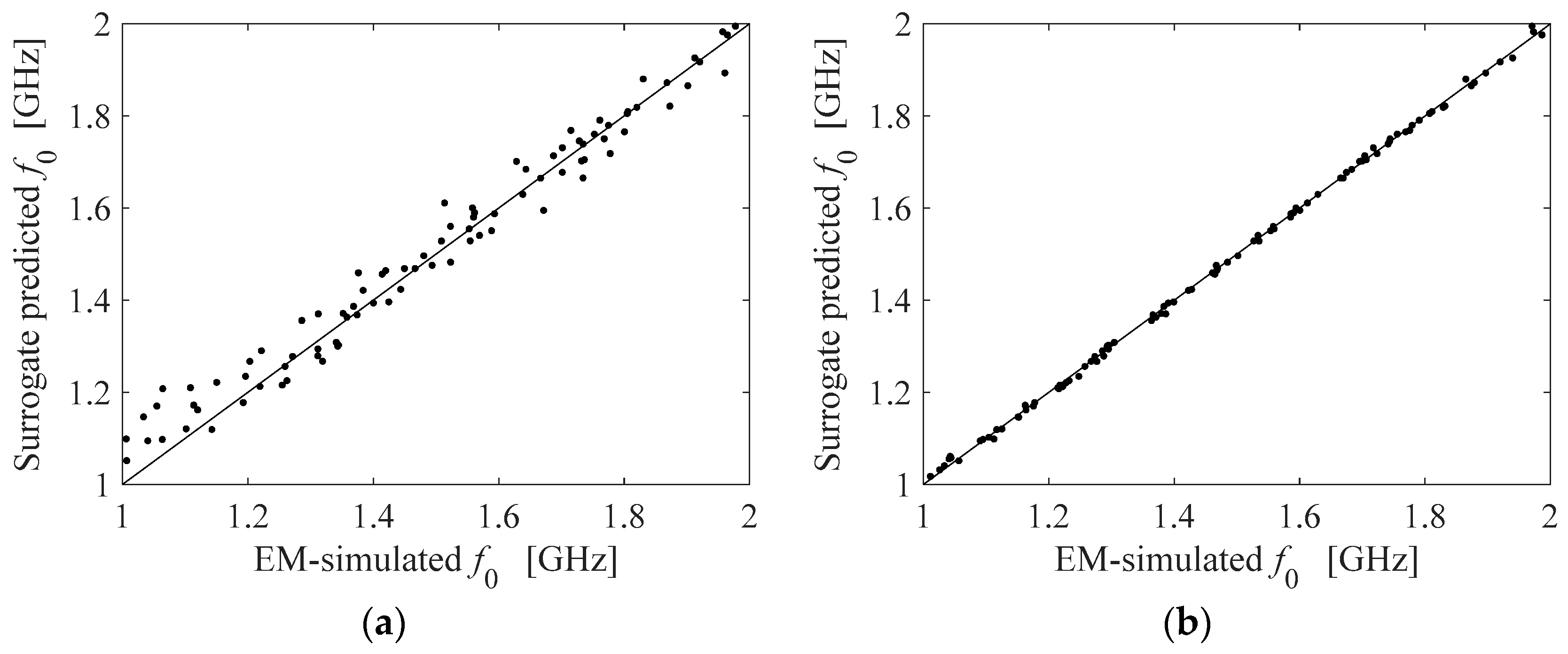
Feature-based no-reference-design modeling (this work)	Modeling error *	f0	2.38%	1.34%	1.09%	0.87%	0.66%	0.55%
		S21(f0)	1.11%	0.77%	0.68%	0.60%	0.55%	0.38%
		S31(f0)	1.70%	1.46%	1.14%	0.99%	1.02%	0.72%
	Cost #		136	166	216	316	516	916

^& The relative RMS error. * The relative RMS error of the relevant coordinate of the response features. ^$ The cost includes reference design acquisition cost (779 EM analyses). ^# The cost includes observable generation (116 EM analyses).

,

Table 5. Circuit II: Modeling results and benchmarking.

Modeling Method				Number of Training Samples
			20	50	100	200	400	800
Kriging	Modeling error &		66.8%	52.3%	38.3%	31.0%	27.3%	23.3%
	Cost		20	50	100	200	400	800
RBF	Modeling error &		64.2%	51.8%	40.5%	37.4%	32.8%	27.2%
	Cost		20	50	100	200	400	800
ANN	Modeling error &		51.4%	29.9%	22.2%	15.2%	10.5%	9.8%
	Cost		20	50	100	200	400	800
CNN	Modeling error &		70.6%	51.9%	39.9%	30.7%	19.7%	11.5%
	Cost		20	50	100	200	400	800
Ensemble learning	Modeling error &		72.1%	53.1%	44.4%	41.6%	38.7%	33.3%
	Cost		20	50	100	200	400	800
Nested kriging [81]	Modeling error &		16.8%	10.0%	7.4%	6.8%	5.1%	4.8%
	Cost $		1034	1064	1114	1214	1414	1814
No-reference-design modeling [82]	Modeling error &		12.8%	7.6%	6.2%	4.7%	4.5%	3.4%
	Cost #		246	276	326	426	626	1026
Feature-based no-reference-design modeling (this work)	Modeling error *	f0	3.66%	1.07%	1.00%	0.57%	0.50%	0.42%
		S21(f0)	0.92%	0.84%	0.70%	0.66%	0.55%	0.51%
		S31(f0)	1.39%	0.96%	0.77%	0.70%	0.65%	0.61%
	Cost #		246	276	326	426	626	1026

^& The relative RMS error. * The relative RMS error of the relevant coordinate of the response features. ^$ The cost includes reference design acquisition cost (1014 EM analyses). ^# The cost includes observable generation (226 EM analyses).

and

Table 6. Circuit III: Modeling results and benchmarking.

Modeling Method				Number of Training Samples
			20	50	100	200	400	800
Kriging	Modeling error &		77.0%	63.6%	53.8%	45.2%	40.0%	35.1%
	Cost		20	50	100	200	400	800
RBF	Modeling error &		79.2%	68.9%	55.2%	43.9%	40.8%	37.2%
	Cost		20	50	100	200	400	800
ANN	Modeling error &		44.1%	36.7%	33.2%	24.6%	20.8%	20.3%
	Cost		20	50	100	200	400	800
CNN	Modeling error &		102.8%	89.6%	44.7%	26.0%	17.8%	15.8%
	Cost		20	50	100	200	400	800
Ensemble learning	Modeling error &		63.5%	47.8%	40.6%	38.1%	36.2%	33.6%
	Cost		20	50	100	200	400	800
Nested kriging [81]	Modeling error &		41.6%	32.3%	19.2%	18.1%	15.2%	12.9%
	Cost $		943	973	1023	1123	1323	1723
No-reference-design modeling [82]	Modeling error &		63.8%	23.7%	15.7%	10.8%	7.2%	6.1%
	Cost #		98	128	178	278	478	878
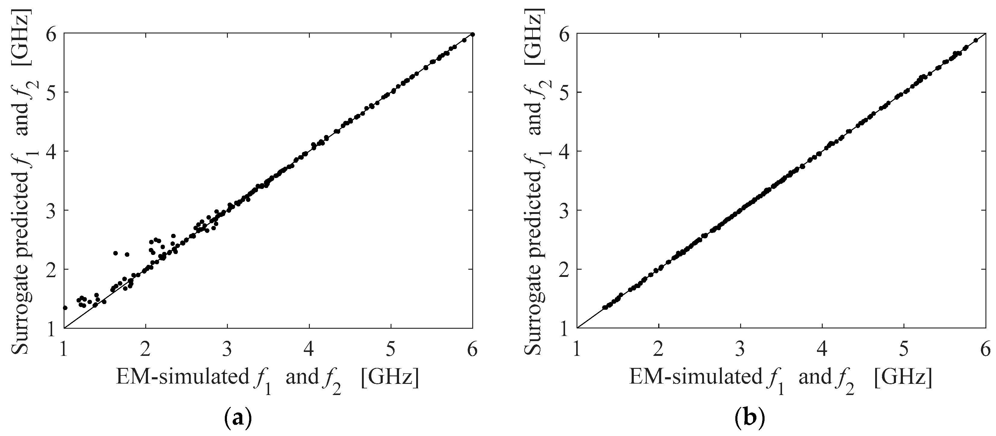
Feature-based no-reference-design modeling (this work)	Modeling error *	f1	2.38%	0.78%	0.49%	0.30%	0.35%	0.27%
		f2	2.00%	0.63%	0.29%	0.23%	0.18%	0.17%
	Cost #		98	128	178	278	478	878

^& The relative RMS error. * The relative RMS error of the relevant coordinate of the response features. ^$ The cost includes reference design acquisition cost (923 EM analyses). ^# The cost includes observable generation (78 EM analyses).

.

For Circuit I, the surrogate model has to be valid across a two-dimensional objective space that includes the following performance figures: operating frequency f₀ within the range from 1.0 GHz to 2.0 GHz and the power split ratio −6 dB ≤ K ≤ 0 dB. Here, minimization of matching and isolation at f₀ and enforcing the required power division ratio at f₀ (see Table 2) are of interest. In the case of Circuit II, the forward model is to cover a two-dimensional objective space with the figures of interest: operating frequency f₀ ∈ (1.0 GHz, 2.0 GHz) and the permittivity ε_r of the substrate within the range of interest from 2.0 to 5.0. The design optimality is defined as for Circuit I, i.e., we aim at minimizing matching and isolation at f₀ and maintaining the equal power split at f₀ (see Table 2). For Circuit III, the performance figures include lower and upper operating frequencies f₁ and f₂, respectively (the latter set using the ratio K_f = f₂/f₁). Here, the aim is to minimize matching and isolation at both operating frequencies; an equal power division ratio is an effect of the structure symmetry.

For Circuit I and Circuit II, we have gathered N_r = 100 random vectors, which required performing 116 and 226 EM simulations, respectively, whereas in the case of Circuit III, gathering 78 EM analyses allowed for obtaining N_r = 50 observables. The accepted samples have been employed to set up the inverse regression surrogate. Next, six sets of training samples of cardinalities N_B = 20, 50, 100, 200, 400, and 800 have been allocated in the respective confined domains.

Table 4, Table 5 and Table 6 gather numerical data: the cost of building the surrogate and modeling accuracy (a relative RMS error assessed using 100 independent test samples). Observe that the overall cost of assembling the nested kriging modeling framework also includes the overhead related with the reference design acquisition: 779, 1014, and 923 EM simulations of the relevant structure, whereas for the proposed approach, the expenditures associated with collecting the observables (116, 226, and 78 EM analyses) add to the overall cost.

In the case of the modeling techniques targeting the complete component responses (i.e., the benchmark methods: kriging, RBF, ANN, CNN, ensemble learning, nested kriging, and no-reference-design modeling), the accuracies are evaluated as ||R(x) − R_s(x)||/||R(x)||, where R and R_S refer to the EM-evaluated and modeled responses, respectively, whereas in the case of the proposed modeling technique, which operates on the response features, the modeling accuracies of the relevant response features are given. For Circuits I and II (see Table 4 and Table 5), the following features are taken into account: the operating frequency f₀, as well as the level coordinates S₂₁(f₀) and S₃₁(f₀), which serve to assess the power split of the circuit. As for Circuit III, in Table 6, the accuracy of both operating frequencies f₁ and f₂ is provided. Furthermore,

Table 7. Absolute errors of the performance figures for Circuits I and II.

Verification Structure	Modeling Error	Number of Training Samples
		20	50	100	200	400	800
Circuit I	f0 [GHz]	0.031	0.019	0.016	0.011	0.010	0.008
	K [dB]	0.235	0.198	0.155	0.139	0.131	0.095
Circuit II	f0 [GHz]	0.046	0.015	0.014	0.008	0.007	0.006
	K [dB]	0.187	0.149	0.128	0.120	0.103	0.095
Circuit III	f1 [GHz]	0.039	0.015	0.010	0.008	0.007	0.005
	f2 [GHz]	0.054	0.018	0.009	0.008	0.006	0.005

provides the absolute error of the performance figures of interest for each verification structure, i.e., the power division and operational frequency for Circuits I and II and the operating frequencies for Circuit III.

The main reason for including the absolute error values is that for the test samples featuring the power split value close to zero, the relative RMS error is not an adequate error quantifier. This is because the RMS error value is evaluated as |K − K_S|/|K|, with K and K_s being the power split calculated based on the extracted features of the EM-simulated response and predicted by the surrogate, respectively. Thus, the value of the said error becomes very large when K ≈ 0, regardless of the actual value of the absolute error, however small. Observe that the absolute power split errors provided in Table 7 for Circuits I and II are minor (fractions of decibel).

The results obtained for Circuit I are shown in Figure 3, Figure 4 and Figure 5. Figure 6 and Figure 7 show the results for Circuit II, whereas Figure 8 and Figure 9 present the results obtained for Circuit III. Figure 3, Figure 4, Figure 6 and Figure 8 present the scatter plots of the performance figures of interest for all considered circuits (i.e., the operational frequency and the power division for Circuit I, the operating frequency for Circuit II, as well as the operating frequencies for Circuit III). Observe that the correlation between the modeled and EM-evaluated results is satisfactory, even for the surrogate built with only 20 training data samples, whereas for two hundred samples it is exceptionally good. Furthermore, Figure 5, Figure 7 and Figure 9 show the EM-simulated frequency characteristics of Circuits I, II, and III, respectively, at the selected test locations of different operating frequencies with the corresponding response features rendered by the proposed surrogate. For all structures, all operating frequencies are predicted accurately, and the same pertains to the power split, wherever relevant.

In our work, the following response features are considered. For couplers, we take into account the power split ratio and the operating frequency, whereas in the case of a power divider, operating frequencies are modeled. However, in the case of couplers and power dividers, the phase is often considered so as to ensure that the required phase difference between the circuit’s ports is maintained at a specified frequency or over a bandwidth. The phase has not been taken into account in the presented approach. Nevertheless, it is possible to include it in the modeling process, which will be carried out in future work.

The modeling accuracy of the introduced feature-based confined surrogates overwhelmingly surpasses that of the conventional models (kriging, RBF, ANN, CNN, and ensemble learning). The same pertains to two performance-driven modeling methods processing entire frequency characteristics: the nested kriging and observable-based modeling techniques. The excellent accuracy of the representation of the operating frequency of all structures, expressed as the relative RMS error, is below five percent even for the training datasets comprising as few as 20 samples, whereas for 50 data samples it goes down to around one percent for all circuits. This degree of modeling accuracy is beyond the capability of the conventional techniques. The data acquisition cost is remarkably low even when taking into account the cost of collecting the random observables required to identify the inverse surrogate: the accuracies of the operational frequencies of around one percent (1.34%, 1.07%, and 0.70% for Circuits I, II, and III, respectively) have been achieved using 166, 276, and 128 data samples, respectively.

It should be emphasized that although the presented modeling approach has been demonstrated using passive microwave circuits, its applicability is not limited to this type of device. In particular, it can be useful for modeling of active circuits, either to represent EM simulations thereof or even measured characteristics. An example of such a device is the power amplifier (e.g., [100]), for which surrogate modeling might be a viable alternative to expensive measurements or complex full-wave electromagnetic analysis in the design context.

Furthermore, it should be reiterated that, using formulation, the proposed modeling approach is independent of the operating frequency of the circuit at hand. As part of our future work, it will be applied to a broader range of circuits, including those that operate at frequencies beyond 10 GHz, as well as circuits implementing a larger variety of functionalities, such as multi-band devices.

4. Conclusions

This article proposed a novel cost-effective feature-based modeling framework that has been applied for assessing vital features from the design perspective of three microwave devices: a rat-race coupler, a branch-line coupler, and a power divider. In the presented approach, the surrogate domain is constricted to encompass only high-quality designs based on a collection of random observables. The incorporation of the problem-specific knowledge embedded in the circuit responses in the form of response features permits us to obtain remarkable accuracy regarding operational frequencies and power division. For all verification structures, the constructed surrogates cover extended ranges of geometry, material, and operating parameters, which are important from the standpoint of their design utility. Our approach surpasses all the benchmark techniques, both conventional and performance-driven ones, in terms of the obtained accuracy and the computational expenditures associated with model setup. This corroborates that a combination of cost-efficient observable-based domain confinement and feature-based modeling leads to significant cost savings. At the same time, it allows for maintaining excellent predictive power of the surrogate.

Moreover, the response features encode in a direct manner information pertaining to vital performance figures such as operating frequencies, which, in conventional frameworks have to be extracted from the circuit outputs. Therefore, despite carrying out the modeling process solely on the layer of features instead of the complete responses, no information pertinent to the design objectives is lost. The presented technique may be considered as an alternative to standard modeling frameworks, in particular, for low-cost rendition of reusable surrogates permitting increased-speed redesign of microwave circuits for distant operational frequencies and/or material parameters.

References

- Cano, J.L.; Ceccato, G.; Fernandez, T.; Mediavilla, A.; Perregrini, L. An ultra-compact full-band waveguide quadrature hybrid coupler. IEEE Microw. Wirel. Comp. Lett. 2022, 32, 9–12. [Google Scholar] [CrossRef]
- Han, J.-H.; Ju, S.-H.; Kang, N.-W.; Lee, W.-S.; Choi, J.-S. Wideband coupling modeling analysis by arbitrarily incoming source fields based on the electromagnetic topology technique. IEEE Trans. Microw. Theory Tech. 2019, 67, 28–37. [Google Scholar] [CrossRef]
- Stanovov, V.V.; Khodenkov, S.A.; Popov, A.M.; Kazakovtsev, L.A. The automatic design of multimode resonator topology with evolutionary algorithms. Sensors 2022, 22, 1961. [Google Scholar] [CrossRef]
- Ghimire, J.; Diba, F.D.; Kim, J.-H.; Choi, D.-Y. Vivaldi antenna arrays feed by frequency-independent phase shifter for high directivity and gain used in microwave sensing and communication applications. Sensors 2021, 21, 6091. [Google Scholar] [CrossRef] [PubMed]
- Aghayari, H.; Nourinia, J.; Ghobadi, C.; Mohammadi, B. Realization of dielectric loaded waveguide filter with substrate integrated waveguide technique based on incorporation of two substrates with different relative permittivity. AEU—Int. J. Electr. Comm. 2018, 86, 17–24. [Google Scholar] [CrossRef]
- Dong, Y.; Yang, B.; Yu, Z.; Zhou, J. Robust fast electromagnetic optimization of SIW filters using model-based deviation estimation and Jacobian matrix update. IEEE Access 2020, 8, 2708–2722. [Google Scholar] [CrossRef]
- Merenda, M.; Felini, C.; Della Corte, F.G. A monolithic multisensor microchip with complete on-chip RF front-end. Sensors 2018, 18, 110. [Google Scholar] [CrossRef]
- Bogdan, G.; Sobolewski, J.; Bajurko, P.; Yashchyshyn, Y.; Oklej, J.; Ostaszewski, D. A wire-bonded patch antenna for millimeter wave applications. Electronics 2023, 12, 632. [Google Scholar] [CrossRef]
- Slimi, M.; Jmai, B.; Dinis, H.; Gharsallah, A.; Mendes, P.M. Metamaterial Vivaldi antenna array for breast cancer detection. Sensors 2022, 22, 3945. [Google Scholar] [CrossRef]
- Przesmycki, R.; Bugaj, M. Crescent microstrip antenna for LTE-U and 5G systems. Electronics 2022, 11, 120. [Google Scholar] [CrossRef]
- Ahmad, S.; Ijaz, U.; Naseer, S.; Ghaffar, A.; Qasim, M.A.; Abrar, F.; Parchin, N.O.; See, C.H.; Abd-Alhameed, R. A jug-shaped CPW-fed ultra-wideband printed monopole antenna for wireless communications networks. Appl. Sci. 2022, 12, 821. [Google Scholar] [CrossRef]
- Zhao, Q.; Wu, Y.; Zhao, X.; Cao, Y.; Chang, C.-H. A 1036-F2/Bit high reliability temperature compensated cross-coupled comparator-based PUF. IEEE Trans. VLSI Syst. 2020, 28, 1449–1460. [Google Scholar] [CrossRef]
- Diman, A.A.; Karami, F.; Rezaei, P.; Amn-e-Elahi, A.; Mousavirazi, Z.; Denidni, C.-H.; Kishk, A.A. Efficient SIW-feed network suppressing mutual coupling of slot antenna array. IEEE Trans. Antennas Propag. 2021, 69, 6058–6063. [Google Scholar] [CrossRef]
- Zakharov, A.; Rozenko, S.; Ilchenko, M. Two types of trisection bandpass filters with mixed cross-coupling. IEEE Microw. Wirel. Comp. Lett. 2018, 28, 585–587. [Google Scholar] [CrossRef]
- Li, S.; Li, S.; Yuan, J. A Compact fourth-order tunable bandpass filter based on varactor-loaded step-impedance resonators. Electronics 2023, 12, 2539. [Google Scholar] [CrossRef]
- Kim, J.; Mauludin, M.F.; Azzahra, H.A.; Jhon, H.; Lee, S.; Cho, K. An 18–19.2 GHz voltage-controlled oscillator with a compact varactor-only capacitor array. Electronics 2023, 12, 1532. [Google Scholar] [CrossRef]
- Lian, W.X.; Yong, J.K.; Chong, G.; Churchill, K.K.P.; Ramiah, H.; Chen, Y.; Mak, P.-I.; Martins, R.P. A reconfigurable hybrid RF front-end rectifier for dynamic PCE enhancement of ambient RF energy harvesting systems. Electronics 2023, 12, 175. [Google Scholar] [CrossRef]
- Roshani, S.; Roshani, S. A compact coupler design using meandered line compact microstrip resonant cell (MLCMRC) and bended lines. Wirel. Netw. 2021, 27, 677–684. [Google Scholar] [CrossRef]
- Socuéllamos, J.M.; Dionisio, R.; Letizia, R.; Paoloni, C. Experimental validation of phase velocity and interaction impedance of meander-line slow-wave structures for space traveling-wave tubes. IEEE Trans. Microw. Theory Tech. 2021, 69, 2148–2154. [Google Scholar] [CrossRef]
- Xiong, Y.; Tang, X.; Ma, J.; Yu, L. Miniaturized metamaterial-inspired travelling wave tube for S band. Electronics 2023, 12, 3062. [Google Scholar] [CrossRef]
- Karpuz, C.; Cakir, M.; Gorur, A.K.; Gorur, A. Design of N-way Wilkinson power dividers with new Input/Output arrangements for power-halving operations. Appl. Sci. 2023, 13, 6852. [Google Scholar] [CrossRef]
- Xu, H.; Zhao, W.-S.; Wang, D.-W.; Liu, J. Compact folded SSPP transmission line and its applications in low-pass filters. IEEE Photonics Tech. Lett. 2022, 34, 591–594. [Google Scholar] [CrossRef]
- Liu, Y.; Wu, W.; Li, J.; Zhao, M.; Wei, F. A balanced BPF with wide bandwidth and steep selectivity based on slotline stub loaded resonators (SSLRs). Electronics 2023, 12, 3389. [Google Scholar] [CrossRef]
- Zeng, Z.; Yao, Y.; Zhuang, Y. A wideband common-mode suppression filter with compact-defected ground structure pattern. IEEE Trans. Electromagn. Compat. 2015, 57, 1277–1280. [Google Scholar] [CrossRef]
- Cao, Z.; Liu, Y.; Liang, C.; Majid, I. Design of UWB filtering impedance transformers and power dividers using stepped-impedance resonators. Electronics 2023, 12, 2800. [Google Scholar] [CrossRef]
- Wu, H.-W.; Chiu, C.-T. Design of compact multi-layered quad-band bandpass filter. IEEE Microw. Wirel. Comp. Lett. 2016, 26, 879–881. [Google Scholar] [CrossRef]
- Gao, M.; Zhao, X. Design of tri-band patch antenna with enhanced bandwidth and diversity pattern for indoor wireless communication. Appl. Sci. 2022, 12, 7445. [Google Scholar] [CrossRef]
- Chen, L.; Qin, M.; Zou, L.; Zhang, T. A low-RCS 2D multi-layer Van Atta array at X-band. Electronics 2023, 12, 3486. [Google Scholar] [CrossRef]
- Ilyas, S.; Shoaib, N.; Nikolaou, S.; Cheema, H.M. A wideband tunable power divider for SWIPT systems. IEEE Access 2020, 8, 30675–30681. [Google Scholar] [CrossRef]
- Wang, Z.; Lang, T.; Qiu, Y. Wideband airy beam generation using reflective metasurfaces with both phase and amplitude modulation. Photonics 2023, 10, 426. [Google Scholar] [CrossRef]
- Fu, C.; Fang, W.; Fan, R.; Wang, L.; Huang, W.; Zhang, Y.; Liu, C. Design and implementation of low parasitic inductance bias circuit for high-power pulsed power amplifiers. Electronics 2023, 12, 1430. [Google Scholar] [CrossRef]
- Iqbal, A.; Tiang, J.J.; Wong, S.K.; Wong, S.W.; Mallat, N.K. QMSIW-based single and triple band bandpass filters. IEEE Trans. Circuits Syst. II Express Briefs 2021, 68, 2443–2447. [Google Scholar] [CrossRef]
- Li, F.; You, B. Complementary multi-band dual polarization conversion metasurface and its RCS reduction application. Electronics 2022, 11, 1645. [Google Scholar] [CrossRef]
- Basit, A.; Daraz, A.; Khan, M.I.; Zubir, F.; A. AlQahtan, S.; Zhang, G. Design and modelling of a compact triband passband filter for GPS, WiMAX, and satellite applications with multiple transmission zero’s. Fractal Fract. 2023, 7, 511. [Google Scholar] [CrossRef]
- Roshani, S.; Roshani, S. Design of a compact LPF and a miniaturized Wilkinson power divider using aperiodic stubs with harmonic suppression for wireless applications. Wirel. Netw. 2020, 26, 1493–1501. [Google Scholar] [CrossRef]
- Ma, Y.; Yang, H.; Wang, J.; Zhu, Y.; Pan, C.; Wu, X. Circular polarization annular leaky-wave antenna with conical and broadside beams. Electronics 2023, 12, 2761. [Google Scholar] [CrossRef]
- Bizan, M.S.; Naseri, H.; Pourmohammadi, P.; Melouki, N.; Iqbal, A.; Denidni, T.A. Dual-band dielectric resonator antenna with filtering features for microwave and mm-wave applications. Micromachines 2023, 14, 1236. [Google Scholar] [CrossRef] [PubMed]
- Soliman, E.A.; Bakr, M.H.; Nikolova, N.K. Accelerated gradient-based optimization of planar circuits. IEEE Trans. Antennas Propag. 2005, 53, 880–883. [Google Scholar] [CrossRef]
- Rajagopalan, H.; Kovitz, J.M.; Rahmat-Samii, Y. MEMS reconfigurable optimized E-shaped patch antenna design for cognitive radio. IEEE Trans. Ant. Propag. 2014, 62, 1056–1064. [Google Scholar] [CrossRef]
- Chen, Z.; Cui, H.; Wu, E.; Yu, X. Computation and communication efficient adaptive federated optimization of federated learning for Internet of Things. Electronics 2023, 12, 3451. [Google Scholar] [CrossRef]
- Torun, H.M.; Swaminathan, M. High-dimensional global optimization method for high-frequency electronic design. IEEE Trans. Microw. Theory Tech. 2019, 67, 2128–2142. [Google Scholar] [CrossRef]
- Shao, K.; Fu, H.; Wang, B. An efficient combination of genetic algorithm and particle swarm optimization for scheduling data-intensive tasks in heterogeneous cloud computing. Electronics 2023, 12, 3450. [Google Scholar] [CrossRef]
- Yu, L.; Ren, J.; Zhang, J. A Quantum-based beetle swarm optimization algorithm for numerical optimization. Appl. Sci. 2023, 13, 3179. [Google Scholar] [CrossRef]
- Premkumar, M.; Jangir, P.; Sowmya, R. MOGBO: A new Multiobjective Gradient-Based Optimizer for real-world structural optimization problems. Knowl.-Based Syst. 2021, 218, 106856. [Google Scholar] [CrossRef]
- Güneş, F.; Uluslu, A.; Mahouti, P. Pareto optimal characterization of a microwave transistor. IEEE Access 2020, 8, 47900–47913. [Google Scholar] [CrossRef]
- Wang, Z.; Qin, J.; Hu, Z.; He, J.; Tang, D. Multi-objective antenna design based on BP neural network surrogate model optimized by improved sparrow search algorithm. Appl. Sci. 2022, 12, 12543. [Google Scholar] [CrossRef]
- Hong, T.; Zheng, S.; Liu, R.; Zhao, W. Design of mmWave directional antenna for enhanced 5G broadcasting coverage. Sensors 2021, 21, 746. [Google Scholar] [CrossRef]
- Zhao, Q.; Sarris, C.D. Space–time adaptive modeling and shape optimization of microwave structures with applications to metasurface design. IEEE Trans. Microw. Theory Tech. 2022, 70, 5440–5453. [Google Scholar] [CrossRef]
- Istenes, G.; Pusztai, Z.; Kőrös, P.; Horváth, Z.; Friedler, F. Kriging-assisted multi-objective optimization framework for electric motors using predetermined driving strategy. Energies 2023, 16, 4713. [Google Scholar] [CrossRef]
- Chen, M.; Gao, X.; Chen, C.; Guo, T.; Xu, W. A comparative study of meta-modeling for response estimation of stochastic nonlinear MDOF systems using MIMO-NARX models. Appl. Sci. 2022, 12, 11553. [Google Scholar] [CrossRef]
- Zhang, Z.; Cheng, Q.S.; Chen, H.; Jiang, F. An efficient hybrid sampling method for neural network-based microwave component modeling and optimization. IEEE Microw. Wirel. Comp. Lett. 2020, 30, 625–628. [Google Scholar] [CrossRef]
- Katkevičius, A.; Plonis, D.; Damaševičius, R.; Maskeliūnas, R. Trends of microwave devices design based on Artificial Neural Networks: A review. Electronics 2022, 11, 2360. [Google Scholar] [CrossRef]
- Jamshidi, M.; Lalbakhsh, A.; Mohamadzade, B.; Siahkamari, H.; Hadi Mousavi, S.M. A novel neural-based approach for design of microstrip filters. AEU—Int. J. Electron. Comm. 2019, 110, 152847. [Google Scholar] [CrossRef]
- Jamshidi, M.; Yahya, S.I.; Roshani, S.; Chaudhary, M.A.; Ghadi, Y.Y.; Roshani, S. A fast surrogate model-based algorithm using multilayer perceptron neural networks for microwave circuit design. Algorithms 2023, 16, 324. [Google Scholar] [CrossRef]
- Plonis, D.; Katkevičius, A.; Krukonis, A.; Šlegerytė, V.; Maskeliūnas, R.; Damaševičius, R. Predicting the frequency characteristics of hybrid meander systems using a feed-forward backpropagation network. Electronics 2019, 8, 85. [Google Scholar] [CrossRef]
- Znou, Q.; Wang, Y.; Jiang, P.; Shao, X.; Choi, S.-K.; Hu, J.; Cao, L.; Meng, X. An active learning radial basis function modeling method based on self-organization maps for simulation-based design problems. Knowl.-Based Syst. 2017, 131, 10–27. [Google Scholar]
- Yang, P.; Wang, T.; Yang, H.; Meng, C.; Zhang, H.; Cheng, L. The performance of electronic current transformer fault diagnosis model: Using an improved whale optimization algorithm and RBF neural network. Electronics 2023, 12, 1066. [Google Scholar] [CrossRef]
- Chen, Y.; Tian, Y.; Qiang, Z.; Xu, L. Optimisation of reflection coefficient of microstrip antennas based on KBNN exploiting GPR model. IET Microw. Antennas Propag. 2018, 12, 602–606. [Google Scholar] [CrossRef]
- Ni, W.; Zhang, Y.; Li, X.; Wang, X.; Wu, Y.; Liu, G. A study on the relationship between RPE and sEMG in dynamic contraction based on the GPR method. Electronics 2022, 11, 691. [Google Scholar] [CrossRef]
- Yu, M.; Liang, J.; Wu, Z.; Yang, Z. A twofold infill criterion-driven heterogeneous ensemble surrogate-assisted evolutionary algorithm for computationally expensive problems. Knowl.-Based Syst. 2022, 236, 107747. [Google Scholar] [CrossRef]
- Wei, Y.; Qi, G.; Wang, Y.; Yan, N.; Zhang, Y.; Feng, L. Efficient microwave filter design by a surrogate-model-assisted decomposition-based multi-objective evolutionary algorithm. Electronics 2022, 11, 3309. [Google Scholar] [CrossRef]
- Wang, X.; Wang, G.G.; Song, B.; Wang, P.; Wang, Y. A novel evolutionary sampling assisted optimization method for high dimensional expensive problems. IEEE Tran. Evol. Comp. 2019, 23, 815–827. [Google Scholar] [CrossRef]
- Forrester, A.I.J.; Keane, A.J. Recent advances in surrogate-based optimization. Prog. Aerosp. Sci. 2009, 45, 50–79. [Google Scholar] [CrossRef]
- Siddiqui, M.U.A.; Qamar, F.; Kazmi, S.H.A.; Hassan, R.; Arfeen, A.; Nguyen, Q.N. A study on multi-antenna and pertinent technologies with AI/ML approaches for B5G/6G networks. Electronics 2023, 12, 189. [Google Scholar] [CrossRef]
- Lahiani, M.A.; Raida, Z.; Veselý, J.; Olivová, J. Pre-design of multi-band planar antennas by artificial neural networks. Electronics 2023, 12, 1345. [Google Scholar] [CrossRef]
- Siddiqui, S.; Azarm, S.; Gabriel, S. A modified Benders decomposition method for efficient robust optimization under interval uncertainty. Struct. Multidiscip. Optim. 2011, 44, 259–275. [Google Scholar] [CrossRef]
- Garbaya, A.; Kotti, M.; Fakhfakh, M.; Tlelo-Cuautle, E. Metamodelling techniques for the optimal design of low-noise amplifiers. Electronics 2020, 9, 787. [Google Scholar] [CrossRef]
- Tan, X.; Sun, J.; Lin, F. A compact frequency-reconfigurable rat-race coupler. IEEE Microw. Wirel. Comp. Lett. 2020, 30, 665–668. [Google Scholar] [CrossRef]
- Choi, J.-S.; Min, B.-C.; Kim, M.-J.; Kumar, S.; Choi, H.-C.; Kim, K.-W. Design of a common-mode rejection filter using dumbbell-shaped defected ground structures based on equivalent circuit models. Electronics 2023, 12, 3230. [Google Scholar] [CrossRef]
- Koziel, S.; Bandler, J.W.; Cheng, Q.S. Reduced-cost microwave component modeling using space-mapping-enhanced EM-based kriging surrogates. Int. J. Numer. Model. 2013, 26, 275–286. [Google Scholar] [CrossRef]
- Feng, F.; Zhang, J.; Zhang, W.; Zhao, Z.; Jin, J.; Zhang, Q. Coarse- and fine-mesh space mapping for EM optimization incorporating mesh deformation. IEEE Microw. Wirel. Comp. Lett. 2019, 29, 510–512. [Google Scholar] [CrossRef]
- Zhang, Y.; Zhang, X.; Liu, L.; Yan, S.; Wang, W.; Jiao, W.; Xu, M.; Hu, W. Multi-objective optimization design of a radial-tangential built-in combined permanent magnet pole generator for electric vehicles. Electronics 2023, 12, 2911. [Google Scholar] [CrossRef]
- Yan, S.; Qian, F.; Li, C.; Wang, J.; Wang, X.; Liu, W. Improved empirical formula modeling method using neuro-space mapping for coupled microstrip lines. Micromachines 2023, 14, 1600. [Google Scholar] [CrossRef]
- Salarkaleji, M.; Eskandari, M.; Chen, J.C.-M.; Wu, C.-T.M. Frequency and polarization-diversified linear sampling methods for microwave tomography and remote sensing using electromagnetic metamaterials. Electronics 2017, 6, 85. [Google Scholar] [CrossRef]
- Pérez, R.; Pelletier, A.; Grenier, J.-M.; Cros, J.; Rancourt, D.; Freer, R. Comparison between space mapping and direct FEA optimizations for the design of Halbach array PM motor. Energies 2022, 15, 3969. [Google Scholar] [CrossRef]
- Wang, X.; Li, T.; Yan, S.; Wang, J. Analytical separated neuro-space mapping modeling method of power transistor. Micromachines 2023, 14, 426. [Google Scholar] [CrossRef]
- Sans, M.; Selga, J.; Velez, P.; Rodriguez, A.; Bonache, J.; Boria, V.; Mrtin, F. Automated design of common-mode suppressed balanced wideband bandpass filters by means of aggressive space mapping. IEEE Trans. Microw. Theory Tech. 2015, 63, 3896–3908. [Google Scholar] [CrossRef]
- Gu, P.; Cao, Z.; He, Z.; Ding, D. Design of ultrawideband RCS reduction metasurface using space mapping and phase cancellation. IEEE Microw. Antennas Propag. Lett. 2023, 22, 1386–1390. [Google Scholar] [CrossRef]
- Xiangjun, X.; Dagang, F.; Yan, D. Frequency space-mapped neuromodeling technique exploiting S-B AFS for the design of microwave circuits. In Proceedings of the Asia-Pacific Microwave Conference, Suzhou, China, 4–7 December 2005; p. 3. [Google Scholar]
- Koziel, S.; Sigurðsson, A.T. Triangulation-based constrained surrogate modeling of antennas. IEEE Trans. Antennas Propag. 2018, 66, 4170–4179. [Google Scholar] [CrossRef]
- Koziel, S.; Pietrenko-Dabrowska, A. Performance-based nested surrogate modeling of antenna input characteristics. IEEE Trans. Antennas Propag. 2019, 67, 2904–2912. [Google Scholar] [CrossRef]
- Koziel, S.; Pietrenko-Dabrowska, A.; Ullah, U. Low-cost modeling of microwave components by means of two-stage inverse/forward surrogates and domain confinement. IEEE Trans. Microw. Theory Tech. 2021, 69, 5189–5202. [Google Scholar] [CrossRef]
- Koziel, S.; Pietrenko-Dabrowska, A. Reliable data-driven modeling of high-frequency structures by means of nested kriging with enhanced design of experiments. Eng. Comput. 2019, 36, 2293–2308. [Google Scholar] [CrossRef]
- Pietrenko-Dabrowska, A.; Koziel, S. Surrogate modeling of impedance matching transformers by means of variable-fidelity electromagnetic simulations and nested cokriging. Int. J. RF Microw. CAE 2020, 30, e22268. [Google Scholar] [CrossRef]
- Koziel, S.; Pietrenko-Dabrowska, A. Low-cost data-driven modelling of microwave components using domain confinement and PCA-based dimensionality reduction. IET Microw. Antennas Propag. 2020, 14, 1643–1650. [Google Scholar] [CrossRef]
- Koziel, S.; Pietrenko-Dabrowska, A. Low-cost performance-driven modelling of compact microwave components with two-layer surrogates and gradient kriging. AEU—Int. J. Electron. Comm. 2020, 126, 153419. [Google Scholar] [CrossRef]
- Pietrenko-Dabrowska, A.; Koziel, S. Nested kriging with variable domain thickness for rapid surrogate modeling and design optimization of antennas. Electronics 2020, 9, 1621. [Google Scholar] [CrossRef]
- Pietrenko-Dabrowska, A.; Koziel, S. Dimensionality-reduced antenna modeling with stochastically established constrained domain. Knowl.-Based Syst. 2023, 271, 110557. [Google Scholar] [CrossRef]
- Koziel, S.; Çalık, N.; Mahouti, P.; Belen, M.A. Reliable computationally efficient behavioral modeling of microwave passives using deep learning surrogates in confined domains. IEEE Trans. Microw. Theory Tech. 2023, 71, 956–968. [Google Scholar] [CrossRef]
- Koziel, S.; Pietrenko-Dabrowska, A. Expedited variable-resolution surrogate modeling of miniaturized microwave passives in confined domains. IEEE Trans. Microw. Theory Tech. 2022, 70, 4740–4750. [Google Scholar] [CrossRef]
- Koziel, S. Fast simulation-driven antenna design using response-feature surrogates. Int. J. RF Microw. CAE 2015, 25, 394–402. [Google Scholar] [CrossRef]
- Mahouti, P. Application of artificial intelligence algorithms on modeling of reflection phase characteristics of a nonuniform reflectarray element. Int. J. Numer. Model. 2020, 33, e2689. [Google Scholar] [CrossRef]
- Zhang, X.; Xu, X. Solubility predictions through LSBoost for supercritical carbon dioxide in ionic liquids. N. J. Chem. 2020, 44, 20544–20567. [Google Scholar] [CrossRef]
- Pietrenko-Dabrowska, A.; Koziel, S. Fast design closure of compact microwave components by means of feature-based metamodels. Electronics 2021, 10, 10. [Google Scholar] [CrossRef]
- Koziel, S.; Pietrenko-Dabrowska, A. Rapid design centering of multi-band antennas using knowledge-based inverse models and response features. Knowl.-Based Syst. 2022, 252, 109360. [Google Scholar] [CrossRef]
- Pietrenko-Dabrowska, A.; Koziel, S. Generalized formulation of response features for reliable optimization of antenna input characteristics. IEEE Trans. Antennas Propag. 2021, 70, 3733–3748. [Google Scholar] [CrossRef]
- Koziel, S.; Sigurðsson, A.T. Performance-driven modeling of compact couplers in restricted domains. Int. J. RF Microw. CAE 2018, 28, e21296. [Google Scholar] [CrossRef]
- Tseng, C.; Chang, C. A rigorous design methodology for compact planar branch-line and rat-race couplers with asymmetrical T-structures. IEEE Trans. Microw. Theory Tech. 2012, 60, 2085–2092. [Google Scholar] [CrossRef]
- Lin, Z.; Chu, Q.-X. A novel approach to the design of dual-band power divider with variable power dividing ratio based on coupled-lines. Prog. Electromagn. Res. 2010, 103, 271–284. [Google Scholar] [CrossRef]
- Mengozzi, M.; Angelotti, A.M.; Gibiino, G.P.; Florian, C.; Santarelli, C. Joint dual-input digital predistortion of supply-modulated RF PA by surrogate-based multi-objective optimization. IEEE Trans. Microw. Tech. 2022, 70, 35–49. [Google Scholar] [CrossRef]