Abstract
Picks are key components for the mechanized excavation of coal by mining machinery, with their wear state directly influencing the efficiency of the mining equipment. In response to the difficulty of determining the overall wear state of picks during coal-mining production, a data-driven wear state identification model for picks has been constructed through the enhanced optimization of Long Short-Term Memory (LSTM) networks via Bayesian algorithms. Initially, a mechanical model of pick and coal-rock interaction is established through theoretical analysis, where the stress characteristic of the pick is analyzed, and the wear mechanism of the pick is preliminarily revealed. A method is proposed that categorizes the overall wear state of picks into three types based on the statistical relation of the actual wear amount and the limited wear amount. Subsequently, the vibration signals of the cutting drum from a bolter miner that contain the wear information of picks are decomposed and denoised using wavelet packet decomposition, with the standard deviation of wavelet packet coefficients from decomposed signal nodes selected as the feature signals. These feature signals are normalized and then used to construct a feature matrix representing the vibration signals. Finally, this constructed feature matrix and classification labels are fed into the Bayesian-LSTM network for training, thus resulting in the picks wear state identification model. To validate the effectiveness of the Bayesian-LSTM deep learning algorithm in identifying the overall picks wear state of mining machinery, vibration signals from the X, Y, and Z axes of the cutting drum from a bolter miner at the C coal mine in Shaanxi, China, are collected, effectively processed, and then input into deep LSTM and Back-Propagation (BP) neural networks respectively for comparison. The results showed that the Bayesian-LSTM network achieved a recognition accuracy of 98.33% for picks wear state, showing a clear advantage over LSTM, BP network models, thus providing important references for the identification of picks wear state based on deep learning algorithms. This method only requires the processing and analysis of the equipment parameters automatically collected from bolter miners or other mining equipment, offering the advantages of simplicity, low cost, and high accuracy, and providing a basis for a proper picks replacement strategy.
1. Introduction
The advancement of technologies such as the Internet of Things (IoT), 5G, Big Data, Cloud Computing, and Artificial Intelligence (AI) has promoted the integration and innovation of a new generation of information technology and coal-mining machinery technology, providing specific technical approaches for the digital transformation and upgrade of coal-mining equipment. The picks are a key component of coal-mining equipment for mechanized coal extraction, and their wear state directly affects the efficiency of the mining equipment. In the process of cutting coal-rock, the picks crush and cut coal-rock under the action of strong thrust, suffering from severe impact and high stress, and experience intense friction with the coal wall. There is a strong non-linear coupling effect and friction wear behavior between the picks and the coal-rock, which can easily lead to the wear failure of the picks [1]. According to statistics, wear failure accounts for as much as 75–90% of all failure modes of picks [2]. In actual coal-mining production, due to factors such as coal-rock characteristics and different picks’ installation angles, the wear degree of the picks at different positions of the mining equipment’s cutting drum will inevitably vary during the cutting process. For picks that wear out quickly, if they are not replaced in time, this will lead to increased wear on the other picks, seriously affecting the cutting efficiency of mining equipment. Replacing picks immediately requires stopping the operation of mining equipment, which also impacts work efficiency [3,4]. Coal-mining enterprises currently rely mainly on manual experience to decide whether to replace picks, and to prevent work efficiency from being affected by multiple pick replacements, they can only adopt the strategy of replacing all picks of different wear levels at once, leading to significant economic waste [5]. Therefore, if the wear state of the mining machinery picks can be accurately identified, it will not only allow real-time understanding of the wear state of the picks on the cutting drum, ensuring the efficient operation of mining equipment, but could also help to propose a scientific picks replacement strategy, significantly reducing production costs for enterprises.
Many scholars have conducted extensive research on the wear mechanism of picks and the prediction of pick life. Dewangan [6] used an electron microscope and X-ray energy dispersive spectroscopy to scan and analyze the images before and after the wear of the pick, revealing the wear mechanism of the pick and the method of predicting wear volume. Zhang et al. [7] used PFC 3D software 5.0 to simulate the cutting process of the pick, conducted cutting experiments on different coated picks, calculated the mass loss before and after cutting, and then predicted and analyzed the life of the pick. Qin et al. [8] proposed a reliability model for the competitive failure of picks under random load impact by considering the effects of sustained impact, variable rate acceleration degradation, and hard failure threshold changes on pick wear. Tian et al. [9] proposed a degradation model based on the Gamma process to describe the wear and tear of picks on the tunneling machine, realizing the prediction of the remaining life of picks.
In recent years, with the development of sensor technology, some scholars have used machine-learning methods to study the identification of the picks wear state. By studying the features of vibration, acoustic emission, cutting force, power, and current signals during the cutting process of picks, they have obtained indirect indicators reflecting the wear of picks, thus achieving the identification of the picks wear state. Zhang et al. [10,11,12] built experimental devices, extracted triaxial vibration signals, infrared temperature signals, and current signals of picks with different wear degrees during the cutting process, constructed a multi-feature signal sample database for picks with different degrees of wear, and established a pick wear degree identification model based on the BP neural network. Jin et al. [13] used an acoustic emission signal acquisition device to collect signals from cutting four different proportions of coal-rock specimens, applied three-layer wavelet packet decomposition and reconstruction technology to process the signals, and used D-S evidence theory to intelligently identify the degree of picks’ wear.
In summary, regarding the identification of the wear state of picks, existing research focuses on one hand on using statistical methods to calculate the wear volume of picks and predict their lifespan, and on the other hand on identifying the wear state of individual picks based on multi-source information fusion. However, due to the constraints of the underground application environment in coal mines, less attention is paid to the overall wear state evaluation of the picks of mining equipment in coal-mine production. Moreover, in the application of machine-learning methods, the commonly used methods in the existing research are shallow learning algorithms, including Support Vector Machines (SVM), Hidden Markov Models (HMM), and BP neural networks. Compared with deep learning models, traditional machine learning and shallow learning algorithms have obvious disadvantages in terms of data-processing capacity, non-linear processing capabilities, and convergence performance. In addition, the adaptive feature learning characteristic of deep learning methods effectively avoids the limitations of manual feature extraction, gets rid of the dependence on prior knowledge, and has a higher recognition accuracy and model generalization capabilities [14].
To further enhance the efficiency and accuracy of identifying the wear state of picks, this paper proposes a model for identifying the overall wear state of picks based on the Bayesian-LSTM deep learning neural network. The main contributions are as follows:
- (1)
- We employed a theoretical analysis method to establish a mechanical model of pick and coal-rock interaction, analyzing the stress characteristics of the picks and revealing the wear mechanism of the picks. In light of the overall wear characteristics of the picks, we achieved the rapid classification of three types of picks wear state through the statistical relationship between the pick wear amount and the limited pick wear amount.
- (2)
- We used the wavelet packet decomposition method to decompose and denoise the vibration signals from the cutting drum of a bolter miner, which contain extensive picks wear information. We then used the standard deviation of the decomposed signal node wavelet packet coefficients as the feature signals. These feature signals, after normalization, were used to construct a feature matrix representing the vibration signals.
- (3)
- We utilized the Bayesian algorithm for its advantages in handling uncertain data, integrating it into the LSTM network to construct a Bayesian-LSTM network. By inputting the constructed feature matrix and classification labels into the Bayesian-LSTM model for training, the recognition results demonstrated a higher accuracy compared to both LSTM and BP neural networks.
The brief structure of this article is as follows: Section 1 introduces the background of the research content and the importance of the research. Section 2 shows the related work about this topic. Section 3 presents the interaction model of the pick and coal-rock during the cutting process, the overall wear state evaluation index, and the feature signals selection of picks wear based on wavelet packet decomposition. Section 4 introduces the Bayesian-LSTM network model. Section 5 presents the analysis of validation and comparison of results. Section 6 provides the conclusions of this article.
2. Related Work
Based on the above, in the research of picks wear state recognition, the current recognition methods are only conducted within a small sample range. When the data volume is too large, computational difficulties arise, which cannot meet the demand for handling massive data in the recognition of the overall wear state of picks [15,16,17]. Therefore, the utilization of deep learning for recognizing the overall wear state of picks presents a significant advantage. Currently, deep learning algorithms have begun to be used in areas like machine tool wear state recognition. For instance, Huang et al. [18] proposed a new method for tool wear prediction based on a deep convolutional neural network and multi-domain feature fusion, constructing a high-accuracy tool wear prediction model combining adaptive feature fusion and automatic continuous prediction. Furthermore, Ma et al. [19] used milling force signals to establish a tool wear prediction model based on convolutional bidirectional LSTM networks, achieving highly accurate prediction results. On the basis of deep learning models, some researchers have attempted to use optimization algorithms to address the reliance of recognition models on large data samples. Wu et al. [20] optimized LSTM networks using a particle swarm optimization (PSO) algorithm and applied an improved polynomial threshold function to denoise tool acceleration vibration signals, thus achieving tool wear quantity prediction and wear state classification. Due to the picks wear state information typically being a time series signal, certain researchers have employed a 1D convolutional neural network (CNN) for the feature classification of temporal signals in related fields. Abdeljaber et al. [21] presented a compact 1D CNN architecture that integrates feature extraction and classification modules, enabling automatic extraction of optimal image-sensitive features directly from raw acceleration signals, utilized for real-time vibration-induced damage monitoring and localization, with a demonstrated outstanding performance and an exceptionally high computational efficiency. Yuan et al. [22] introduced a 1D CNN model for rapid and accurate comprehensive damage assessment post-earthquake. Their results revealed that the prediction accuracy of the 1D CNN model is comparable to that of 2D CNN models, yet with an over 90% reduced computation time and an over 69% resource usage reduction. Abdoli et al. [23] introduced a 1D CNN-based approach for environmental sound classification that directly captures audio signal patterns through convolutional layers, achieving an average accuracy of 89% with fewer data than traditional feature-based methods.
Through comparative analysis of the use of deep learning methods for tool wear state recognition, it can be observed that most of the recognition models still employ traditional structures such as CNN and LSTM. Some choose to combine optimization algorithms like PSO and Genetic Algorithms (GA) to address convergence problems during weight training. When considering the selection of input parameters, the vast majority of studies still rely on the research experience of their predecessors, without considering the impact of different input parameter combinations on the output results [24,25,26,27]. Additionally, these network models yield fixed weight matrices after training, and these weight matrices are no longer updated. The model cannot allocate different weights based on the change in inputs, so its generalization ability when faced with different tasks can be significantly constrained [28]. The LSTM deep learning network, with its unique memory units and gate mechanisms, is adept at capturing dependencies in time series, offering a distinct advantage in processing temporal data [29,30,31,32]. However, the randomness introduced by environmental factors and parameter choices might compromise the accuracy of the recognition results [33]. In recent years, several researchers have incorporated Bayesian theory into LSTM deep learning networks to estimate weights and biases. This approach shifts the neural network parameter estimation from point estimation to probability distribution, enabling the network to evaluate the certainty or uncertainty of results. Consequently, this enriches the deep learning network’s formidable data-fitting capability, further enhancing its learning precision. Li et al. [34] proposed a method that leverages Bayesian-LSTM to perform Stochastic Variational Inference (SVI) on process-based hydrological models. By constructing a residual model, they sought to refine the predictions of uncertainty in hydrological models. The results demonstrated that this method provided a highly reliable uncertainty interval. Compared to the Bayesian linear regression model, Bayesian-LSTM offered superior uncertainty estimation. Yang et al. [35] introduced a HiBayes-LSTM method containing an FIE component to capture past and future time dependencies. By collecting large-scale HTRO datasets, they extended the weights of the LSTM network to a probabilistic model, ensuring uncertainty in the HM direction of the head trajectory predictions. Experimental outcomes revealed that HiBayes-LSTM notably outperformed nine other methods in predicting ODIs’ significance.
3. Preliminaries
This section analyzes the wear mechanism of picks by establishing a mechanical model of the pick and coal-rock mass, and proposes a classification method for the overall wear state of the picks of mining machinery. At the same time, a method for selecting the characteristic parameters of the picks wear state is provided.
3.1. Pick and Coal-Rock Interaction Model
Picks are the main tools for mining machinery to cut coal-rock. The tip of pick, that is, the top of the alloy head cone, is mainly used to wedge into the coal-rock mass. After the pick wedges into the coal-rock mass, it comes into contact with the coal-rock, and a pick and coal-rock interaction model is shown in Figure 1. The uncut coal-rock mass shows unevenness, some relatively hard and sharp coal-rock particles are pressed into the tip surface under the action of the normal load, and they perform a cutting action on the pick tip during the drum movement process. The long-term reciprocating cutting action causes the material on the pick surface to continuously peel off, thus intensifying the wear of the pick. Therefore, the friction force on the alloy head is the main cause of the wear of the pick tip.
Figure 1.
Interaction model of rotary pick and coal-rock mass.
According to the classic plane-cutting model of pick [36], it is assumed that the friction coefficient between the coal-rock mass and the pick is , and the relationship between the surface pressure stress of the coal-rock mass and its compressive strength is:
where is the semi-cone angle of the pick tip.
The radius of the circular hole of the pick tip in the coal-rock mass can be expressed as follows:
where is the cutting thickness of the pick, and is the tensile stress of the coal-rock mass.
As can be seen from Figure 1, when the pick on the drum is in a rotating cutting state, the cross-section AD perpendicular to the instantaneous cutting speed direction on the pick body is elliptical. Take the differential element AD on the contact surface between the pick and the coal-rock mass for research, denoted as , according to the differential principle:
where is the fracture angle, is the length from the tip to a point on the pick body, and is the radius of the cross-sectional circle.
According to the relative positional relationship, the semi-axes and of the ellipse can be expressed as follows:
where is the cutting angle of the cutting pick.
For ease of analysis, this ellipse is equivalently treated as a circle with a radius of to obtain:
From this, it can be determined that after considering the frictional force and cutting angle, the cutting force element on its conical surface when the pick is rotating and cutting is:
where , , and are the frictional force element, cutting force element, and normal pressure element on the pick surface, respectively.
After integrating Equation (6), the total horizontal force on the conical surface in interaction between the pick and the coal-rock mass is obtained:
As can be seen from Equation (7), the cutting resistance of the pick in the rotating cutting condition is a quadratic function of its cutting thickness, it is directly proportional to the square of the tensile stress of the coal-rock mass and the ratio of the compressive strength, and it has a complex trigonometric function relationship with the cutting angle. The traction resistance of the pick is about (0.5–0.8) , and the lateral force is about (0.1–0.2) .
3.2. Overall Wear State Evaluation Index
As analyzed in the previous section, the interaction between the pick and the coal-rock mass is extremely complex, and its wear types mainly include abrasive wear, erosion wear, and fatigue wear, among which abrasive wear accounts for about 70~75% of the total wear volume. Abrasive wear refers to the phenomenon or process that causes surface material loss during the interaction between abrasives or hard micro-protrusions and the worn material surface. If the removed material is very small, it is usually referred to as micro-cutting. In the abrasive wear process of the pick, the abrasive can remove the pick material in one interaction. Therefore, the micro-cutting abrasive wear theoretical model can be used to study the macroscopic coal-rock cutting process of the pick.
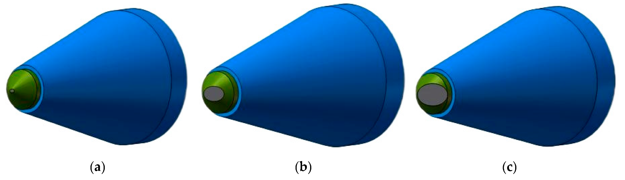
When only considering the wear of the pick tip, the wear trend of the alloy head is shown in Figure 2. As can be seen, the wear of the alloy head is like a plane parallel to the coal-rock surface layer cutting the alloy head. The coal-rock surface continuously laminates the alloy head, while the height of the alloy head being cut gradually increases. When the layer cutting height changes from 1 mm to 3 mm, a significant change in its wear volume occurs, which can be represented by the cross-sectional area of the plane and the alloy head. The larger the wear area, the more wear the alloy head has.
Figure 2.
Trend of pick wear. (a) Slight wear, (b) Moderate wear, (c) Severe wear.
From the above analysis, it can be seen that for the wear of the pick tip, the contact area between the pick and the coal-rock is the main influencing factor. The larger the area of contact between the pick and the coal-rock, the more wear, that is, the more the area of contact between the pick tip and the coal-rock can reflect the wear amount of the pick. Therefore, without considering the self-rotation ability of the pick during the cutting process, the wear coefficient of a single pick can be represented by the following equation:
where is the contact area with the coal-rock, is the limited contact area with the coal-rock, is the layer cutting thickness, and is the limited layer cutting thickness. Based on this, this article proposes to establish an overall wear state coefficient based on the wear coefficient of a single pick and use it to evaluate the overall wear situation of picks, thereby achieving a method of quickly obtaining the overall wear degree of picks during coal-mine production.
where is the total number of each type of pick and is the single pick wear rate. According to the field pick replacement experience of engineering cases, before and after pick replacement, the overall picks wear state can be divided into three levels: slight wear, moderate wear, and severe wear. The range of the overall wear coefficient corresponding to the determined various wear states is shown in Table 1.

Table 1.
Classification of overall picks wear state.
3.3. Selection of Picks Wear Feature Signal
During the cutting process of mining machinery, the tip of the pick bears a high concentrated stress. Due to the small contact area of the pick tip, the picks violently rub against the coal-rock mass during the cutting process and generate vibration, accompanied by the propagation of vibration waves. Under certain cutting parameters, the vibration signals generated by the cutting drum with different global wear levels must be different. Therefore, this article chooses the vibration signal of the cutting drum to effectively identify the overall wear state of picks.
Wavelet packet analysis is a refined signal analysis method that can decompose the collected non-linear parameter signals into different scales, obtain the node features of the signals at each scale, and form a feature parameter group. The principle of extracting pick wear features with wavelet packets is as follows:
The expression of the wavelet packet function is
where is the scale parameter, is the oscillation parameter, is the translation parameter, and is the time variable.
The wavelet packet function satisfies the double scale equation:
In the formula, is the coefficient of the low-pass filter, is the coefficient of the high-pass filter, and is the orthogonal wavelet packet.
The projection of the original parameter signal on , that is, the wavelet packet coefficient is
The algorithm of wavelet packet decomposition is
This article relies on engineering examples to process the cutting vibration signal, compares the node wavelet packet coefficients of the signal with other signal feature parameters, and finally proposes to use the standard deviation of the vibration signal wavelet packet coefficients as a recognition indicator to identify the overall wear state of picks.
The feature vector definition for the overall wear state identification of picks is:
where is the standard deviation of the wavelet packet coefficients of signal at the node , is the k-th wavelet packet coefficient of the signal at the node , and is the average of the wavelet packet coefficients of the signal at the node .
4. Methods
The section illustrates the structure and characteristics of the LSTM neural network, proposes a Bayesian-LSTM neural network optimized by the Bayesian algorithm, and also provides the process of an overall picks wear state recognition model based on wavelet packet decomposition and Bayesian-LSTM.
4.1. LSTM Network
The LSTM deep learning network is a novel type of Recurrent Neural Network (RNN) with its inherent recursive traits. The LSTM model introduces three gates (input gate, forget gate, output gate) to control the historical information transmission between neural units, thereby avoiding the gradient explosion and gradient vanishing problems that may occur in the training process of traditional recursive neural networks [37]. It effectively handles the long-term dependency relationships present in long sequences. The vibration signal data used in this paper are a kind of time series data, which reflect the change trend in the wear condition of the picks over time. Therefore, this paper chooses to use the LSTM network for the state recognition of time series.
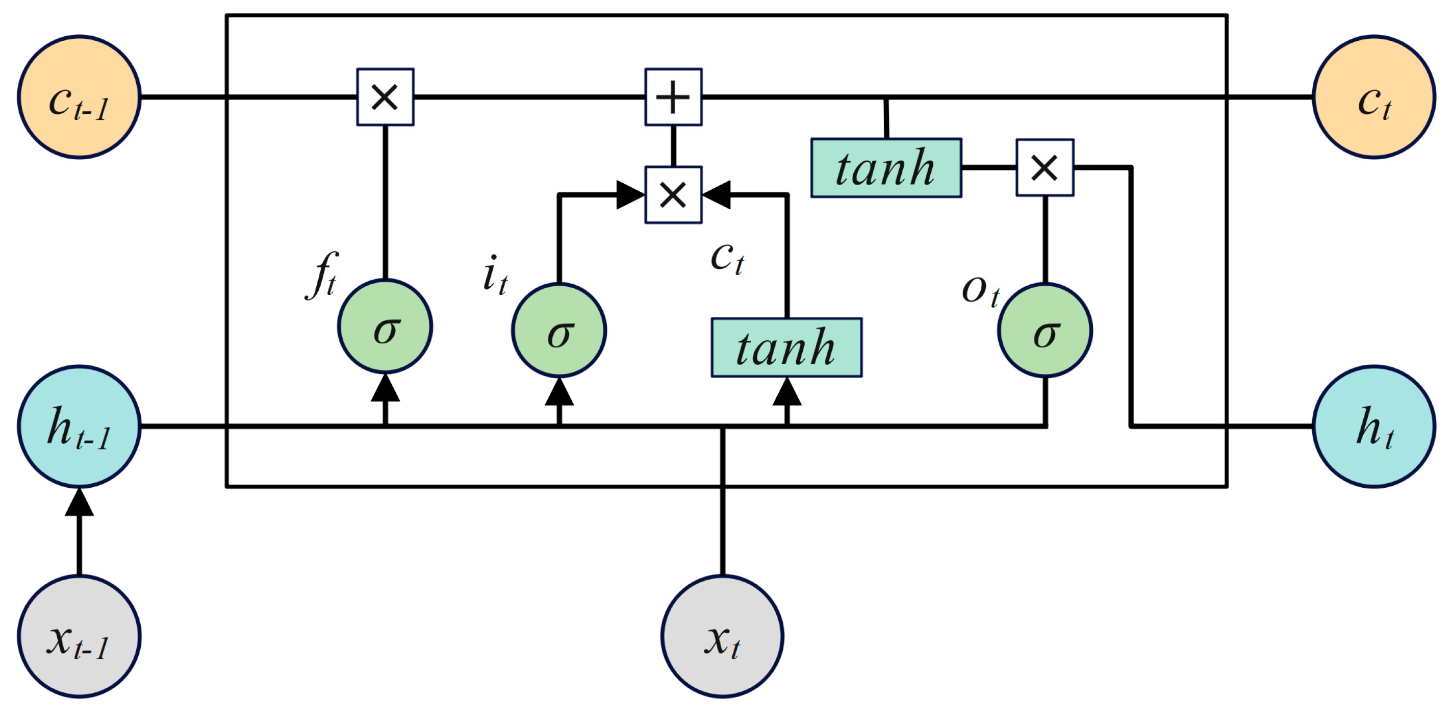
Within the architecture of an LSTM model, every unit holds a cell, which essentially acts as its memory store. The manner in which memory units in an LSTM are read and modified is controlled by three critical components: the input gate, the forget gate, and the output gate. Typically, sigmoid or tanh functions depict their operations. To illustrate, the operational process of an LSTM unit proceeds as such: at each interval, it absorbs two forms of external data-the current state and the preceding LSTM’s hidden state. Additionally, an internal input, the state of the memory unit, is also fed to each gate. Following the receipt of these input data, the gates compute the data from diverse sources, and the outcomes determine their activation status. The input gate’s input is manipulated via a nonlinear function, which then amalgamates with the memory unit state that the forget gate has handled, creating a novel memory unit state. Ultimately, the memory unit state, after being processed by a nonlinear function and dynamically managed by the output gate, becomes the LSTM unit’s output. As a result, LSTM networks possess the capacity to retain long-term dependencies as they can selectively eliminate certain data, maintain beneficial information, and relay it to the subsequent step via the output gate. The basic structure of LSTM is shown in Figure 3.
Figure 3.
The basic structure of LSTM.
The data transfer within the LSTM neural unit follows these equations:
In these equations, , , , are weight matrices connected to the input signal ; , , , are weight matrices connected to the output signal of the hidden layer; , , are diagonal matrices connecting the output vectors of the neuron activation function and gate function; , , , are bias vectors; and is the activation function, usually a tanh or sigmoid function.
4.2. Parameter Optimization Based on Bayesian Theory
The core idea of parameter optimization based on Bayesian theory is to treat LSTM as a Bayesian model, place prior distribution on the network weights and bias parameters of LSTM, and then use variational inference to infer the posterior distribution of the parameters given the data [38].
Bayesian theory considers as a random variable that can be described by a probability distribution. According to Bayes’ formula,
where is the posterior distribution, is the prior distribution, is the evidence or normalization constant, and its calculation formula is as follows:
Since the evidence is in integral form, it is mostly non-integrable except in some ideal situations. Therefore, the method of variational inference is often used, that is, a set of distributions are introduced to approximate the posterior distribution of parameters , denoted as , where is the variational parameter matrix corresponding to the model parameters .
The difference between the original distribution and the variational distribution is generally measured by Kullback–Leibler (KL) divergence:
In this equation, is the Evidence Lower Bound (ELBO). It can be seen that the smaller the divergence, the greater the variational lower bound, indicating that the variational distribution is closer to the original distribution. The maximum value of the evidence lower bound is obtained to obtain the optimal distribution.
The idea of variational inference is to follow the gradient of variational parameters, express the gradient as an expected value, and use the Monte Carlo method to estimate this expectation. An unbiased gradient estimation is obtained by sampling from the variational distribution, which saves the analytical calculation of the variational lower bound. The objective function of variational inference is:
In this equation, is the expectation about , and is the joint distribution of and .
If is the free parameter of , the gradient of the lower bound of the distribution can be expressed as:
According to the Monte Carlo sampling method, the gradient of the variational lower bound is
Therefore, for stochastic variational inference, the execution process of variational inference is
where is the learning rate. When the change in the free parameters is less than a given tolerance, the calculation stops. Based on the inferred network weights and bias parameters from the posterior distribution, the network can continue to train according to the LSTM algorithm.
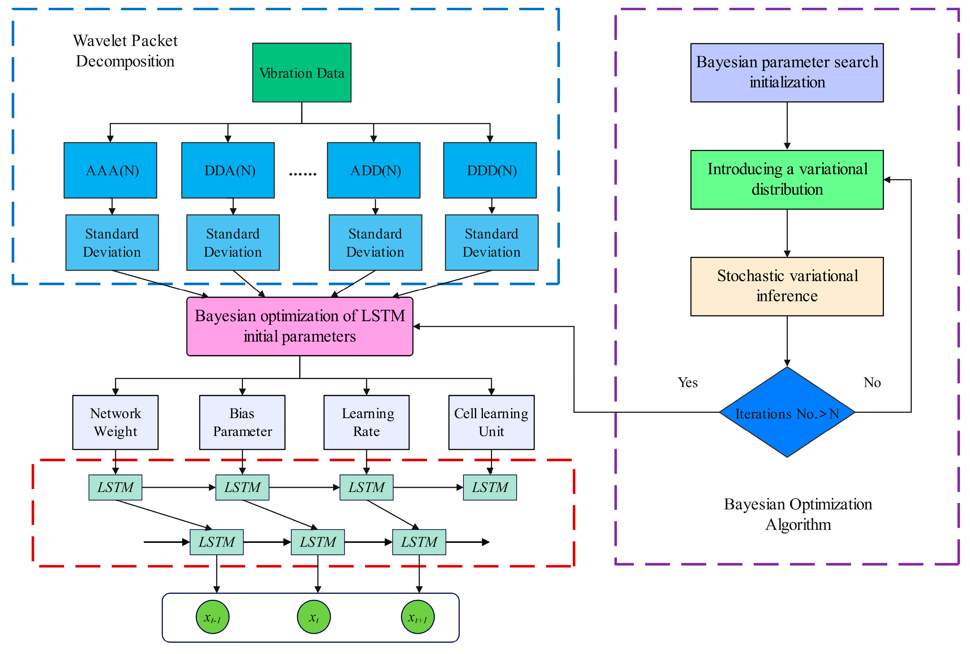
In summary, the proposed picks wear state recognition model is shown in Figure 4, and the process of the picks wear state recognition model based on wavelet packet decomposition and Bayesian optimization of LSTM is as follows:

Figure 4.
The framework of picks wear state recognition model.
- (1)
- Use wavelet packet decomposition to decompose the original signal of cutting vibration, and choose the standard deviation of wavelet packet coefficients as the feature signal of the neural network;
- (2)
- Establish the parameter seeking model of the LSTM network, and use Bayesian optimization theory to optimally seek parameters for the initial parameters of the LSTM network;
- (3)
- Build and initialize the LSTM and fully connected layer network based on the parameter seeking result, and set the hyperparameters of the network;
- (4)
- Train the network on the sample training set, and use the trained network to perform classification testing on the test samples.
5. Engineering Verification
To verify the effectiveness and efficiency of the proposed overall picks wear state recognition model, extensive engineering experiments on real datasets have been implemented against the classic methods under differently labeled rations.
5.1. Data Acquisition
In order to verify the effectiveness of the picks wear recognition method proposed in this article, the real parameters of the bolter miner of Shaanxi C mine in China are selected for verification. The roof of this mine is moderately stable, using a bolter miner for tunneling, the coal seam thickness is about 5 m, and the average daily advance is about 50 m. The properties of coal-rock mass in this mine are relatively stable, and the average daily number of pick replacements is found to be roughly equivalent through statistics, proving that the C mine is quite suitable for conducting picks wear state recognition experiments.
In the experiment, we continued to adopt the strategy of centrally changing the picks. By statistically measuring the wear volume of the picks before each shift, and calculating the overall wear coefficient of the picks on drum cutting according to Formula (9), it was found that if the picks were not replaced for 2 days, the overall wear coefficient could reach 0.3. If extended to more than 3 days, the wear coefficient could reach 0.5. This preliminarily proved that delaying the replacement of picks can accelerate their wear. Therefore, the field collected the X, Y, and Z directional vibration acceleration of the cutting drum of the bolter miner immediately after replacing the picks, and 2 and 3 days later, respectively representing slight wear, moderate wear, and severe wear levels. The vibration sensor location is shown in Figure 5.
Figure 5.
The vibration sensor location on bolter miner.
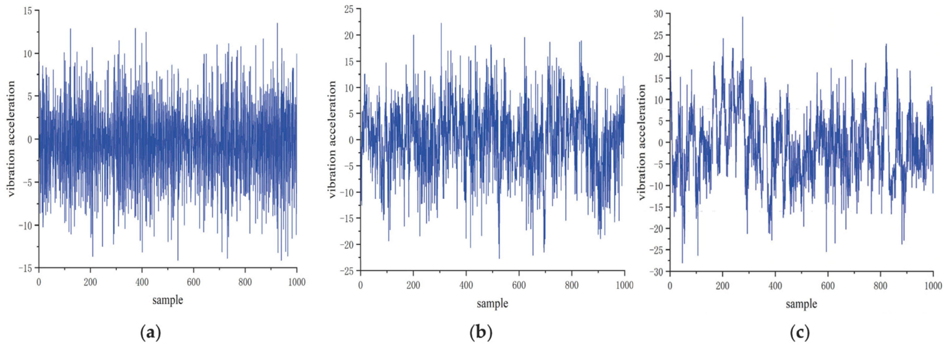
During the field tests, 2 s of X, Y, and Z directional vibration data were recorded every minute under each working condition, ensuring the data collection was in a stable state. In total, 100 sets of data were recorded under each working condition, with a total of two detection tests conducted, forming a total of 600 sets of characteristic data. The collected Y-directional raw vibration data are shown in Figure 6.
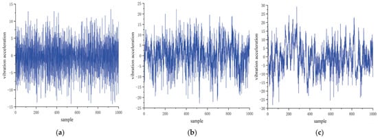
Figure 6.
Y-directional raw vibration data. (a) Slight wear, (b) Moderate wear, (c) Severe wear.
5.2. Data Processing
As can be seen from Figure 6, the amplitude of the drum vibration signal is larger with an increased picks wear degree. In the process of collecting the vibration acceleration curve of the cutting drum, errors may occur due to factors such as the environment and noise, which cause inaccuracy in the signal. Merely utilizing time-domain analysis cannot adequately analyze the vibration signal. To more accurately identify the degree of wear of the cutting picks, this paper converts the acquired time-domain signal into a frequency-domain signal for further analysis to obtain more fitting evaluation parameters.
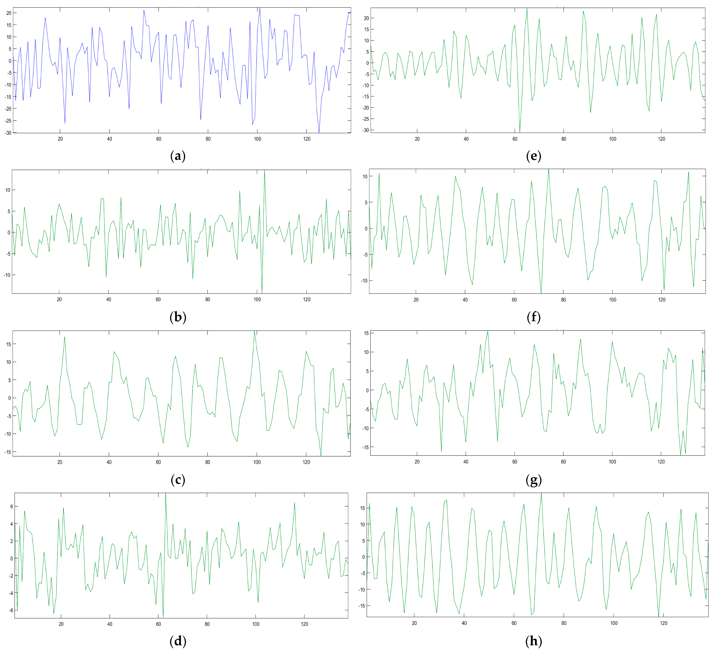
Wavelet packet analysis divides the signal into detailed hierarchical divisions to improve signal processing capabilities. This study chose to perform wavelet packet decomposition on the time-domain signals of the vibration acceleration of the cutting drum under three picks wear states, selecting DB wavelet basis. It was found that when n equals 8, the time-domain waveform of wavelet packet decomposition is the smoothest and the frequency characteristics are ideal; thus, this paper selected DB8 as the wavelet basis. After signal decomposition, each node is respectively recorded as (3, 0), (3, 1), (3, 2), (3, 3), (3, 4), (3, 5), (3, 6), and (3, 7). Figure 7 shows the wavelet packet decomposition diagram of the Y-directional vibration signals of picks with moderate wear.
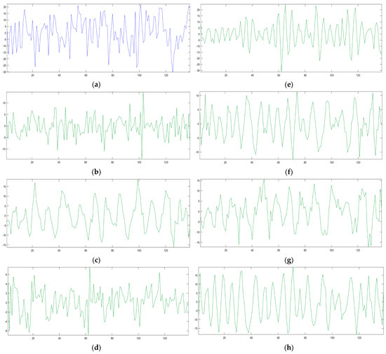
Figure 7.
Wavelet packet decomposition diagram of Y-directional vibration signals for picks with moderate wear. (a) Coefficients of Packet (3, 0), (b) Coefficients of Packet (3, 1), (c) Coefficients of Packet (3, 2), (d) Coefficients of Packet (3, 3), (e) Coefficients of Packet (3, 4), (f) Coefficients of Packet (3, 5), (g) Coefficients of Packet (3, 6), (h) Coefficients of Packet (3, 7).
Based on the wavelet packet decomposition coefficients, the standard deviation of the decomposition wavelet packet coefficients can be obtained according to Formula (14), as shown in Table 2. The above data form a 25 × 600 feature matrix, where the first 24 columns are standard deviations of wavelet packet coefficients, and the last column is the classification label. The process involved randomly selecting 480 groups of data as the training set and 120 groups of data as the test set.
Table 2.
Standard deviations of wavelet packet coefficients for each picks wear state.
5.3. Overall Picks Wear State Recognition Model
Before importing the data, it is necessary to normalize the standard deviation data of the decomposed wavelet packet coefficients, as shown below:
Bayesian-LSTM runs in a Python environment and is built based on the open-source machine learning library PyTorch and the probabilistic model Pyro. The hyperparameter settings are as shown in Table 3.
Table 3.
Hyperparameter settings of the Bayesian-LSTM network.
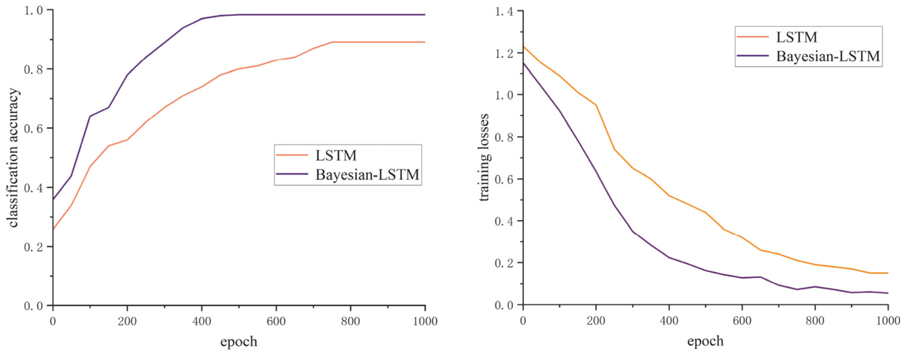
To verify the recognition effect of the Bayesian-LSTM network, a deep LSTM network is chosen for comparison analysis. In the deep LSTM network, the settings of hyperparameters such as the learning rate and the number of hidden layers are consistent. The training results of the two networks are shown in Figure 8.

Figure 8.
Comparison of the training results of the two networks.
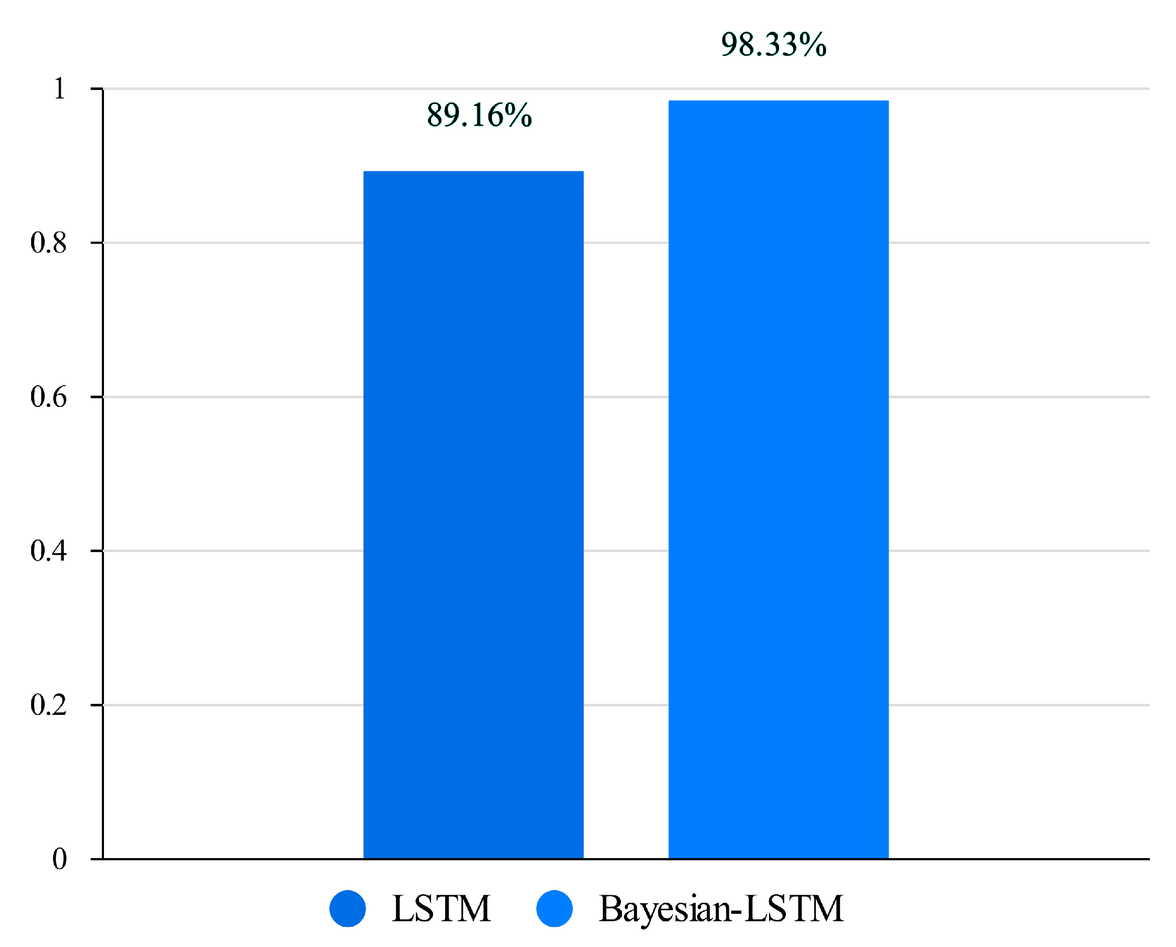
As shown in Figure 8, with the increase in iterations, the Bayesian-LSTM network decreases very quickly. Compared to the standard LSTM network, it achieves a higher accuracy at a faster rate and the accuracy at each measurement point is higher than that of the standard LSTM. To quantify the accuracy of the two prediction models, a comparison of their accuracy rates is shown in Figure 9.

Figure 9.
Comparison of accuracy rates for two networks.
As can be seen from the above figures, given a certain set of hyperparameters, the classification accuracy of the Bayesian-LSTM model is 98.33%, while the LSTM model’s classification accuracy is 89.16%. In the aforementioned conclusions, the recognition accuracy of the LSTM model is relatively low, which is because the weight parameters of the LSTM model are fixed and have not yet been optimized. If we use the Adam algorithm [39] to update and iterate the weights, and use Softmax as the classifier, the final set of hyperparameters for the optimized LSTM recognition model would be as given in Table 4 below.
Table 4.
Hyperparameter settings of the optimized LSTM network.
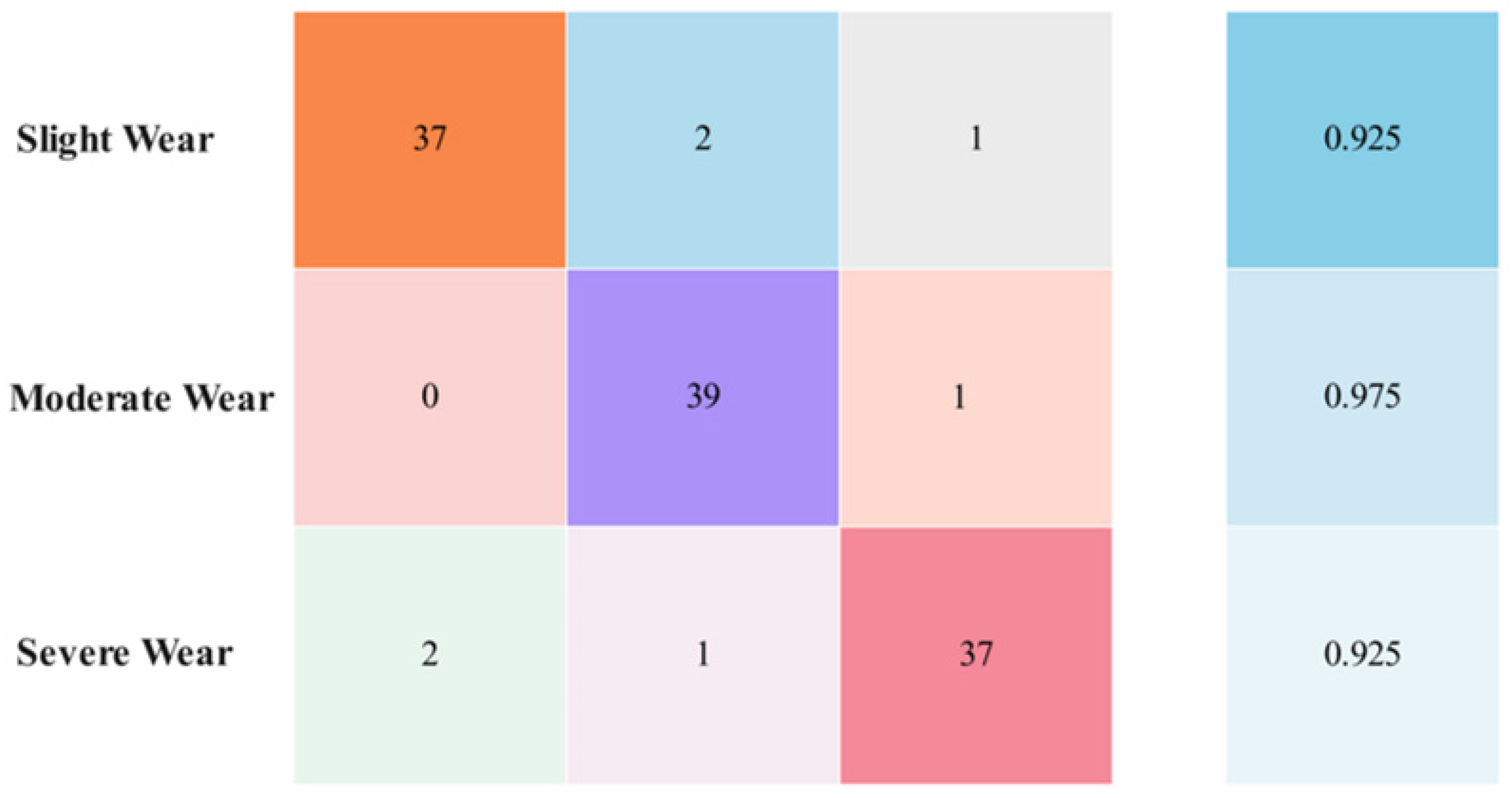
The final confusion matrix of the LSTM network optimized by Adam is shown in Figure 10.
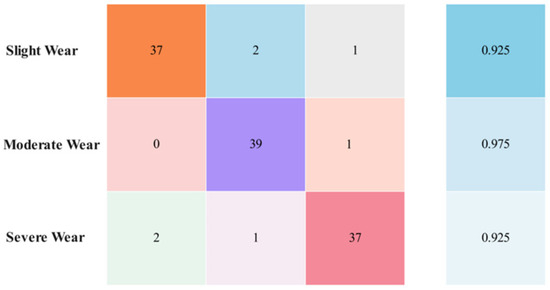
Figure 10.
Confusion matrix with the optimized LSTM network.
In order to further verify the accuracy and generalization ability of the Bayesian-LSTM deep learning network in the recognition of the picks wear state, the obtained results are compared with the classification results of the optimized LSTM and BP networks. The comparison results are as shown in Table 5 below.
Table 5.
Comparison of the accuracy of overall picks wear recognition under different algorithms.
From the table, it can be seen that the recognition accuracy of optimized LSTM and Bayesian-LSTM are higher than that of the BP network, proving that deep learning networks have a better accuracy when dealing with nonlinear data. However, in the macro view, the classification accuracy of the LSTM network on small-sample data is not ideal and has certain limitations. When the Bayesian theory is introduced, the Bayesian-LSTM model effectively reduces the model overfitting caused by sparse data and noise and provides an uncertainty quantification for prediction, effectively improving its recognition accuracy.
6. Conclusions
Accurate identification of the overall picks wear state is a core task in achieving intelligent upgrades of mining equipment. This study utilized theoretical analysis methods to research the mechanical model of the interaction between the pick and the coal-rock, preliminarily revealing the wear mechanism of the cutting picks. Based on this, we proposed a classification judgment method for three types of overall pick wear state. This study proposed an overall picks wear state recognition method based on Bayesian-LSTM. Using the vibration signals of the bolter miner’s cutting drum as the basis for recognition, we used status labels and feature matrices to train the recognition model. The trained Bayesian-LSTM recognition model can effectively recognize the overall picks wear state. Compared to deep LSTM and BP, this method has a higher recognition accuracy.
In conclusion, this method only requires processing and analyzing equipment parameters automatically collected by mining machinery such as a bolter miner during its working process. It has the advantages of being easy to implement, low-cost, and highly accurate, providing a basis for the correct pick replacement strategy. However, there are still several challenging issues in theoretical and practical research, and recommended research works in the future as follows:
- (1)
- It is necessary to research more feature parameters that can reflect the wear state of picks, such as current data on the cutting motor and pressure signals of the hydraulic cylinder.
- (2)
- It is essential to study further efficient signal processing methods that can reduce the data disturbance caused by coal-mine scenes and to further improve the accuracy of picks wear state recognition.
Author Contributions
Conceptualization, D.S. and Y.Z.; writing-original draft preparation, D.S.; visualization, D.S. and Y.Z.; project administration, D.S.; funding acquisition, D.S. All authors have read and agreed to the published version of the manuscript.
Funding
This research was funded by the China National Key R&D Program (Grant No. 2020YFB1314000) and the Research Project Supported by Shanxi Scholarship Council of China (Grant No. 2022-186).
Data Availability Statement
The data used to support the findings of this study are available from the corresponding author upon request.
Acknowledgments
The partial study was completed at the National Engineering Laboratory for Coal Mining and Excavation Machinery Equipment, and the author would like to thank the laboratory for its assistance.
Conflicts of Interest
The authors declare no conflict of interest.
References
- Dogruoz, C.; Bolukbasi, N.; Rostami, J.; Acar, C. An experimental study of cutting performances of worn picks. Rock Mech. Rock Eng. 2016, 49, 213–224. [Google Scholar] [CrossRef]
- Holmberg, K.; Kivikytö-Reponen, P.; Härkisaari, P.; Valtonen, K.; Erdemir, A. Global energy consumption due to friction and wear in the mining industry. Tribol. Int. 2017, 115, 116–139. [Google Scholar] [CrossRef]
- Liu, S.; Ji, H.; Liu, X.; Jiang, H. Experimental research on wear of conical pick interacting with coal-rock. Eng. Fail. Anal. 2017, 74, 172–187. [Google Scholar] [CrossRef]
- Zhao, L.; He, J.; Hu, J.; Liu, W. Effect of pick arrangement on the load of shearer in the thin coal seam. J. China Coal Soc. 2011, 36, 1401–1406. [Google Scholar]
- Krauze, K.; Mucha, K.; Wydro, T.; Pieczora, E. Functional and operational requirements to be fulfilled by conical picks regarding their wear rate and investment costs. Energies 2021, 14, 3696. [Google Scholar] [CrossRef]
- Dewangan, S.; Chattopadhyaya, S. Characterization of wear mechanisms in distorted conical picks after coal cutting. Rock Mech. Rock Eng. 2016, 49, 225–242. [Google Scholar] [CrossRef]
- Zhang, Q.; Fan, Q.; Gao, H.; Wu, Y.; Xu, F. A study on pick cutting properties with full-scale rotary cutting experiments and numerical simulations. PLoS ONE 2022, 17, e0266872. [Google Scholar] [CrossRef]
- Qin, Y.; Zhang, X.; Zeng, J.; Shi, G.; Wu, B. Reliability analysis of mining machinery pick subject to competing failure processes with continuous shock and changing rate degradation. IEEE Trans. Reliab. 2022, 72, 795–807. [Google Scholar] [CrossRef]
- Tian, Y.; Wei, X.; Hao, T.; Jiayao, Z. Study on wear degradation mechanism of roadheader pick. Coal Sci. Technol. 2019, 47, 129–134. [Google Scholar]
- Zhang, Q.; Gu, J.; Liu, J.; Liu, Z.; Tian, Y. Pick wear condition identification based on wavelet packet and SOM neural network. J. China Coal Soc. 2018, 43, 2077–2083. [Google Scholar]
- Zhang, Q.; Zhang, X.; Tian, Y.; Liu, Z. Research on recognition of pick cutting wear degree based on LVQ neural network. Chin. J. Sens. Actuators 2018, 31, 1721–1726. [Google Scholar]
- Zhang, Q.; Yu, W.; Wang, C. Research on identification of pick wear degree of road header based on PNN neural network. Coal Sci. Technol. 2019, 47, 37–44. [Google Scholar]
- Jin, L.; Cao, Y.; Qi, Y.; Yu, T.; Gu, J.; Zhang, Q. Identification of pick wear state based on acoustic emission and DS evidence theory. Coal Sci. Technol. 2020, 48, 120–128. [Google Scholar]
- Lecun, Y.; Bengio, Y.; Hinton, G. Deep learning. Nature 2015, 521, 436–444. [Google Scholar] [CrossRef] [PubMed]
- Su, H.; Qi, W.; Hu, Y.; Sandoval, J.; Zhang, L.; Schmirander, Y.; Chen, G.; Aliverti, A.; Knoll, A.; Ferrigno, G.; et al. Towards mode-free tool dynamic identification and calibration using multi-layer neural network. Sensors 2019, 19, 3636. [Google Scholar] [CrossRef]
- Liu, X.; Jing, W.; Zhou, M.; Li, Y. Multi-scale feature fusion for coal-rock recognition based on completed local binary pattern and convolution neural network. Entropy 2019, 21, 622. [Google Scholar] [CrossRef]
- Achmad, P.; Ryo, F.; Hideki, A. Image based identification of cutting tools in turning-mil1ing machines. J. Jpn. Soc. Precis. Eng. 2019, 85, 159–166. [Google Scholar]
- Huang, Z.; Zhu, J.; Lei, J.; Li, X.; Tian, F. Tool wear predicting based on multi-domain feature fusion by deep convolutional neural network in milling operations. J. Intell. Manuf. 2020, 31, 953–966. [Google Scholar] [CrossRef]
- Ma, J.; Luo, D.; Liao, X.; Zhang, Z.; Huang, Y.; Lu, J. Tool wear mechanism and prediction in milling TC18 titanium alloy using deep learning. Measurement 2021, 173, 108554. [Google Scholar] [CrossRef]
- Wu, F.; Nong, H.; Ma, C. Tool wear prediction method based on particle swarm optimization long and short time memory model. J. Jilin Univ. 2023, 53, 989–997. [Google Scholar]
- Abdeljaber, O.; Avci, O.; Kiranyaz, S.; Gabbouj, M.; Inman, D.J. Real-time vibration-based structural damage detection using one-dimensional convolutional neural networks. J. Sound Vib. 2017, 388, 154–170. [Google Scholar] [CrossRef]
- Yuan, X.; Tanksley, D.; Li, L.; Zhang, H.; Chen, G.; Wunsch, D. Faster post-earthquake damage assessment based on 1D convolutional neural networks. Appl. Sci. 2021, 11, 9844. [Google Scholar] [CrossRef]
- Abdoli, S.; Cardinal, P.; Koerich, A. End-to-end environmental sound classification using a 1D convolutional neural network. Expert Syst. Appl. 2019, 136, 252–263. [Google Scholar] [CrossRef]
- Zhu, Q.; Li, H.; Wang, Z.; Chen, J.F.; Wang, B.J.P.S.T. Short-term wind power forecasting based on LSTM. Power Syst. Technol. 2017, 41, 3797–3802. [Google Scholar]
- Brili, N.; Ficko, M.; Klanènik, S. Automatic identification of tool wear based on thermography and a convolutional neural network during the turning process. Sensors 2021, 21, 1917. [Google Scholar] [CrossRef] [PubMed]
- Casado-Vara, R.; Martin del Rey, A.; Pérez-Palau, D.; de-la-Fuente-Valentín, L.; Corchado, J.M. Web traffic time series forecasting using LSTM neural networks with distributed asy nchronous training. Mathematics 2021, 9, 421. [Google Scholar] [CrossRef]
- Yang, T.; Chen, J.; Deng, H.; Lu, Y. UAV abnormal state detection model based on timestamp slice and multi-separable CNN. Electronics 2023, 12, 1299. [Google Scholar] [CrossRef]
- Bie, F.; Du, T.; Lyu, F.; Pang, M.; Guo, Y. An integrated approach based on improved CEEMDAN and LSTM deep learning neural network for fault diagnosis of reciprocating pump. IEEE Access 2021, 9, 23301–23310. [Google Scholar] [CrossRef]
- Marani, M.; Zeinali, M.; Songmene, V.; Mechefske, C.K. Tool wear prediction in high-speed turning of a steel alloy using long short-term memory modelling. Measurement 2021, 177, 109329. [Google Scholar] [CrossRef]
- Najafi, M.; Jalali, S.M.E.; KhaloKakaie, R.; Forouhandeh, F. Prediction of cavity growth rate during underground coal gasification using multiple regression analysis. Int. J. Coal Sci. Technol. 2015, 2, 318–324. [Google Scholar] [CrossRef]
- Gers, F.; Sshmidhuber, J.; Cummins, F. Learning to forget: Continual prediction with LSTM. Neural Comput. 2000, 12, 2451–2471. [Google Scholar] [CrossRef] [PubMed]
- Schoot, R.; Depaoli, S.; King, R.; Kramer, B.; Märtens, K.; Tadesse, M.G.; Vannucci, M.; Gelman, A.; Veen, D.; Willemsen, J.; et al. Bayesian statistics and modelling. Nat. Rev. Methods Primers 2021, 1, 1. [Google Scholar] [CrossRef]
- Song, Y.; Zhang, J.; Zhao, X.; Wang, J. An accelerator for semi-supervised classification with granulation selection. Electronics 2023, 12, 2239. [Google Scholar] [CrossRef]
- Li, D.; Marshall, L.; Liang, Z.; Sharma, A.; Zhou, Y. Bayesian LSTM with stochastic variational inference for estimating model uncertainty in process-based hydrological models. Water Resour. Res. 2021, 57, e2021WR029772. [Google Scholar] [CrossRef]
- Yang, L.; Xu, M.; Guo, Y.; Deng, X.; Gao, F.; Guan, Z. Hierarchical Bayesian LSTM for head trajectory prediction on omnidirectional images. IEEE Trans. Pattern Anal. Mach. Intell. 2021, 44, 7563–7580. [Google Scholar] [CrossRef] [PubMed]
- Evans, I. A theory of the cutting force for point-attack picks. Int. J. Rock Mech. Min. Sci. 1984, 2, 67–71. [Google Scholar] [CrossRef]
- Hocheiter, S.; Schmidhuber, J. Long short-term memory. Neural Comput. 1997, 9, 1735–1780. [Google Scholar] [CrossRef]
- Wu, X.; Marshall, L.; Sharma, A. The influence of data transformations in simulating total suspended solids using Bayesian inference. Environ. Model. Softw. 2019, 121, 104493. [Google Scholar] [CrossRef]
- Kingma, D.; Ba, J. Adam: A method for stochastic optimization. arXiv 2014, arXiv:1412.6980. [Google Scholar]


Disclaimer/Publisher’s Note: The statements, opinions and data contained in all publications are solely those of the individual author(s) and contributor(s) and not of MDPI and/or the editor(s). MDPI and/or the editor(s) disclaim responsibility for any injury to people or property resulting from any ideas, methods, instructions or products referred to in the content. |
© 2023 by the authors. Licensee MDPI, Basel, Switzerland. This article is an open access article distributed under the terms and conditions of the Creative Commons Attribution (CC BY) license (https://creativecommons.org/licenses/by/4.0/).