A Study on the Rapid Detection of Steering Markers in Orchard Management Robots Based on Improved YOLOv7

Abstract

In order to guide the orchard management robot to realize autonomous steering in the row ends of a complex orchard environment, this paper proposes setting up steering markers in the form of fruit trees at the end of the orchard rows and realizing the rapid detection of the steering markers of the orchard management robot through the fast and accurate recognition and classification of different steering markers. First, a high-precision YOLOv7 model is used, and the depthwise separable convolution (DSC) is used instead of the 3 × 3 ordinary convolution, which improves the speed of model detection; at the same time, in order to avoid a decline in detection accuracy, the Convolutional Block Attention Module (CBAM) is added to the model, and the Focal loss function is introduced to improve the model’s attention to the imbalanced samples. Second, a binocular camera is used to quickly detect the steering markers, obtain the position information of the robot to the steering markers, and determine the starting point position of the robot’s autonomous steering based on the position information. Our experiments show that the average detection accuracy of the improved YOLOv7 model reaches 96.85%, the detection time of a single image reaches 15.47 ms, and the mean value of the localization error is 0.046 m. Comparing with the YOLOv4, YOLOv4-tiny, YOLOv5-s, and YOLOv7 models, the improved YOLOv7 model outperforms the other models in terms of combined detection time and detection accuracy. Therefore, the model proposed in this paper can quickly and accurately perform steering marker detection and steering start point localization, avoiding problems such as steering errors and untimely steering, shortening the working time and improving the working efficiency. This model also provides a reference and technical support for research on robot autonomous steering in other scenarios.

1. Introduction

In recent years, in the context of the modern agricultural industrial base and the great development of specialty benefit agriculture, the fruit industry has been developing rapidly, and the advantageous industries have become more prominent [1,2,3]. At present, with the expanding area of orchard planting and the rapid development of orchard agricultural equipment autonomy and intelligence, orchard management robots, which can carry out tasks such as inspection, spraying, weeding, picking, and handling, and many other areas have been widely used [4,5,6]. At the same time, autonomous steering is an important part of the unmanned agricultural transporter in relation to orchard operation; minimizing driving time and driving distance while improving the operational efficiency of the vehicle in the steering process is the focus of many researchers at present [7,8]. However, the orchard environment is complex; GPS/BDS can be easily blocked by fruit trees, leading to losses in positioning information and making the autonomous steering of on-ground orchard robots a difficult problem. Therefore, this paper proposes an efficient and high-precision steering mark detection method for orchard management robots that provides a theoretical basis for orchard management robots to realize autonomous steering at the end of the rows of fruit trees and is of great significance for realizing the multifunctional intelligent operation of orchard management robots.

To date, many scholars have studied the recognition of marked signs. Qian R et al. [9] designed a template matching method based on a multilevel chain code histogram, and their experimental results show that their feature expression method (based on the multilevel chain code histogram) can effectively improve the recognition effect of triangular, circular, and octagonal signboards, and the computational cost is low, and it can realize real-time recognition of marking boards. Liang M et al. [10] used the “feature representation operator + traditional machine learning” method to convert the original image from RGB color space to grayscale space, used HOG to represent the features, and then fed this into SVM classification. After reading papers from all over the world, we found that the template-based signage matching method is susceptible to breakage, occlusion, and stains, which leads to the general robustness and universality of the algorithm; the combination scheme of the feature representation operator and traditional machine learning complicates grasping the balance of feature representation complexity, classification processing dimensions, and computational resource consumption, so the above method is not applicable to steering signage recognition in complex orchard environments, and it is difficult to apply in the design work of the orchard.

For the positioning of signage, some scholars have also conducted a large number of studies utilizing different methods for the acquisition of location information. Chen Zheng et al. [11] used morphological processing and edge analysis for the coarse location of license plates, which is insufficiently resistant to interference from complex backgrounds and relies heavily on pre-set license plate aspect ratios, which is not generalizable for signage with irregular shapes. Jiang L et al. [12] proposed an image segmentation algorithm with SLIC (Simple Linear Iterative Clustering) super pixel and improved frequency-tuned (FT) saliency detection to localize and segment the digital region of signage. Although the above methods realize the positioning of the signage, they are overly dependent on image features, susceptible to environmental factors such as light, less stable, and have insufficient positioning accuracy. In the orchard, the steering markers are seriously obscured, which increases the difficulty of identifying and localizing the steering markers; therefore, it is necessary to study the visual localization of the steering markers of the orchard management robot in a complex orchard environment.

At present, convolutional neural networks in deep learning are widely used in text, speech, picture, and video [13,14,15]. They show great advantages, especially in target detection tasks, as they can quickly and accurately complete the detection task [16,17,18]. To solve the recognition and localization of steering markers in complex scenarios in orchards, the seventh-generation algorithm YOLOv7 of the regression-based YOLO series was selected for steering mark recognition, and a binocular camera was used as the vision sensor for steering mark localization. Additionally, this paper replaces the 3 × 3 ordinary convolution in the backbone network as well as the feature-enhanced network with depthwise separable convolution on the basis of YOLOv7, introduces the CBAM attention mechanism, and introduces the Focal Loss function for the multi-classification task to make it able to satisfy both the accuracy of the recognition and localization as well as the speed of the detection and compares it with different models to evaluate the performance and effectiveness of the improved model.

2. Materials and Methods

As shown below, the method proposed in this paper consists of two parts: steering marker detection and localization.

The images are captured using a binocular camera and, after they have been captured, they are inputted into the improved YOLOv7 model for steering mark detection.

The steering markers are localized via the parallax method to obtain the 3D position information of the steering markers in the camera coordinate system.

2.1. Dataset Production

2.1.1. Data Acquisition

The images used in this study were collected at the Baima test site of Nanjing Agricultural University in Nanjing, Jiangsu Province, China. The source of the collected dataset has two parts. A portion of the image data were captured through static shots using a two-megapixel camera module as the acquisition device. The other part consists of image data intercepted from video frames during the operation of the orchard management robot, using a ZED2i binocular camera as the acquisition device. A total of 874 original images were obtained by uniformly naming and saving the collected images in JPG format. These images include steering marker datasets captured under different working scenes, lighting conditions, and weather conditions. When the orchard management robot is working, if it needs to work between different rows of fruit trees, it needs to make a U-turn. If the robot needs to drive out of the orchard, it needs to turn straight. Therefore, the steering markers are categorized into four types: Turn Left, Turn Right, Turn left and U-turn, Turn right and U-turn. Figure 1 shows the four different signs for the four steering markers. Figure 2 shows the actual working roadmap of the orchard management robot (based on the recognized steering markers).

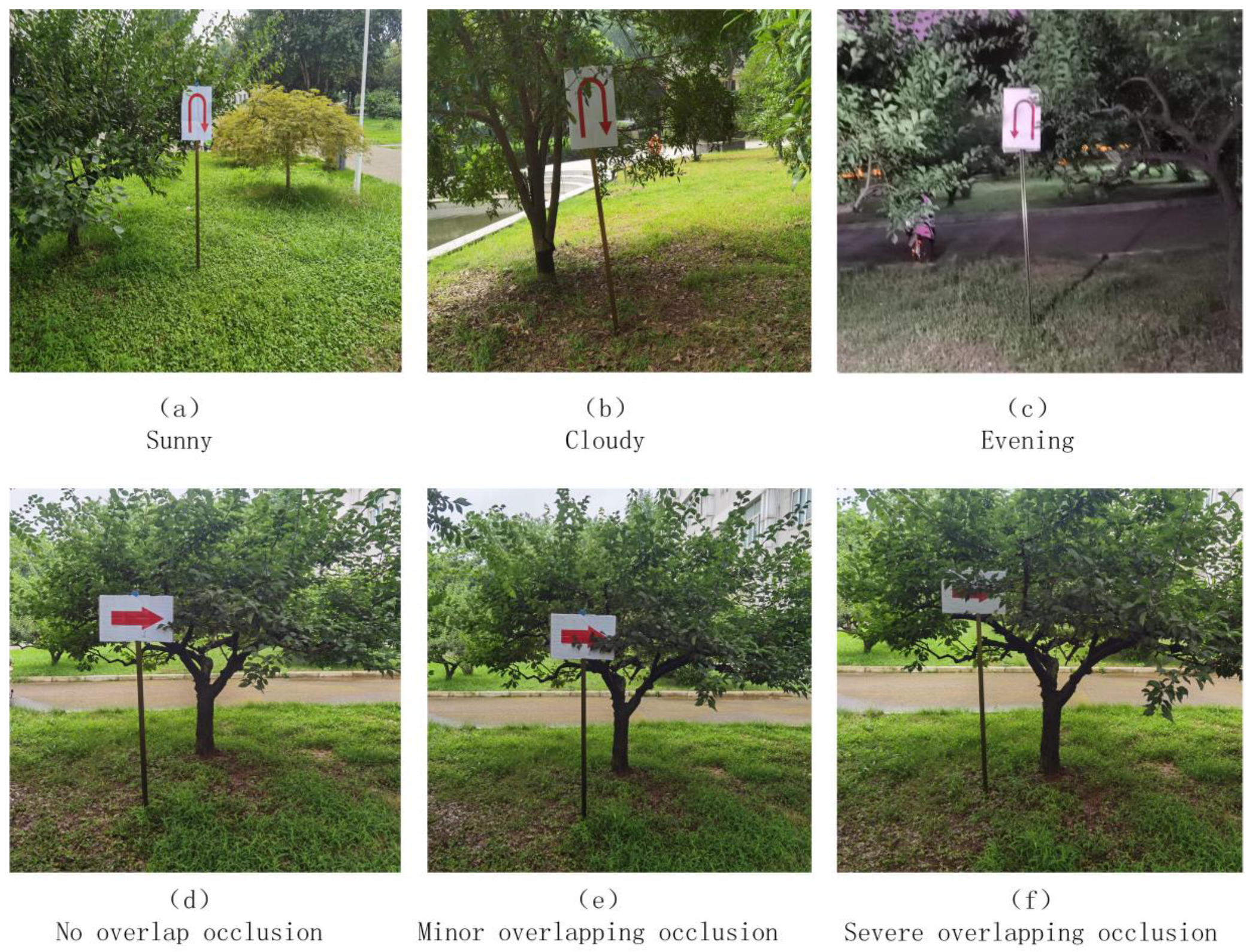
The orchard environment is complex, and the orchard management robot generally works all day long. The changes in external light conditions from day to evening and the overlapping occlusion of fruit tree branches and leaves are diverse. Therefore, this study explores three types of weather, namely sunny, cloudy, and evening, with three overlapping occlusion scenarios, namely no overlapping occlusion, slight overlapping occlusion, and severe overlapping occlusion, as shown in Figure 3 for the steering marking images in the complex scenario.

2.1.2. Data Preprocessing

This study used the annotation tool Labelimg to annotate targets in the annotation format of the Pascal VOC dataset. Among them, the steering marker for a left turn was labeled as “Turn Left”, the marker for a right turn was labeled as “Turn Right”, the marker for a left turn and U-turn was labeled as “Turn left and Turn around”, and the marker for a right turn and U-turn was labeled as “Turn right and Turn around”. The annotation files were generated in the “.xml” format.

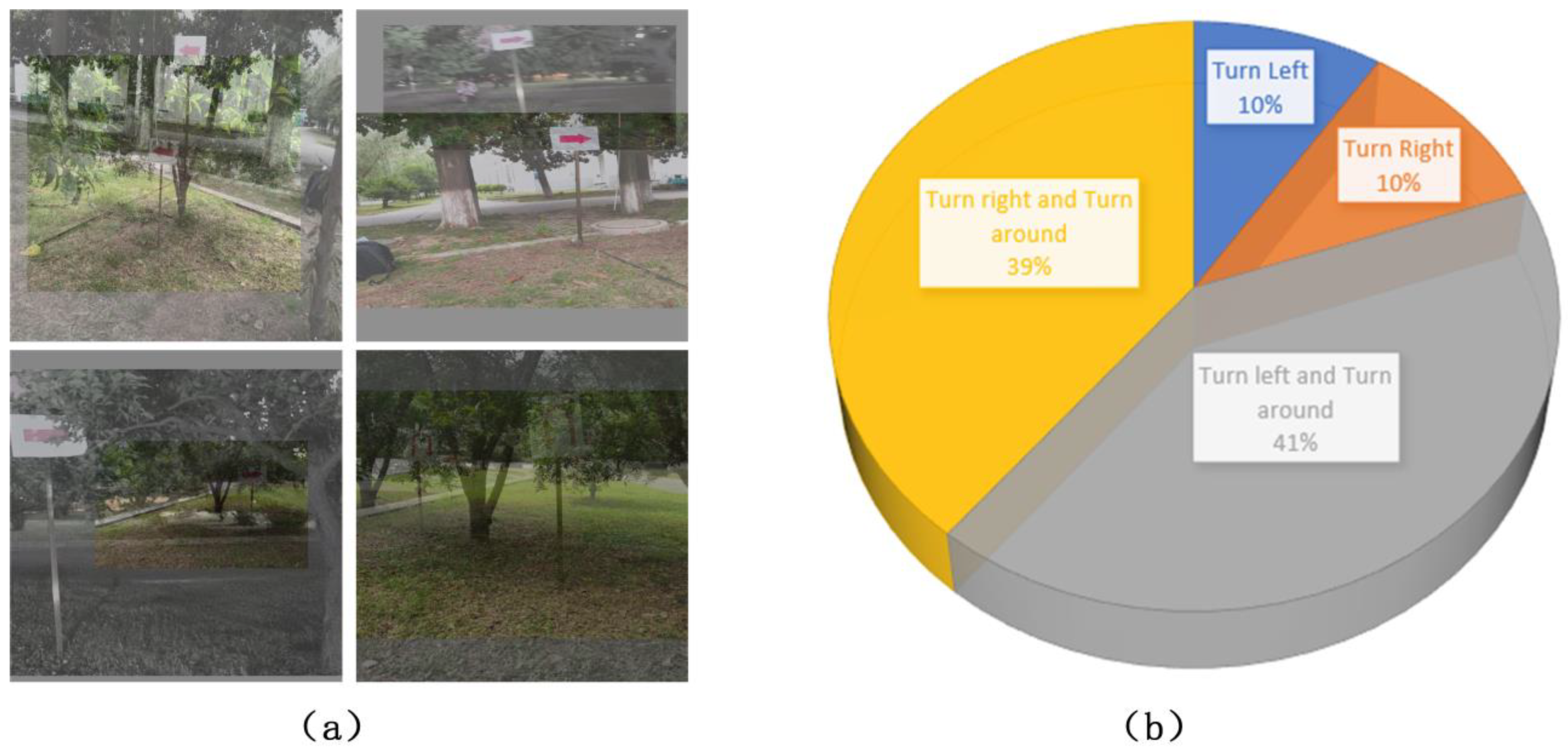
In order to enhance the richness of the experimental dataset, image data enhancement techniques were used to expand the size of the dataset, reduce the dependence of the steering mark recognition model on certain image attributes, reduce the overfitting of the training model, and enhance the stability of the model. In this study, the original 874 images captured were used for Mixup data enhancement. Mixup data enhancement reads two images at a time, and data enhancement processes such as flipping, scaling, and color gamut change were performed on the two images, respectively. Finally, the two photos were stacked together; the enhanced effect is shown in Figure 4a, expanding it to 3373 sheets. After completing data augmentation, it was divided into a training set and a validation set in a 9:1 ratio, where the training set included 3036 images, and the validation set included 337 images. The labeled files of the training set were visualized and analyzed, as shown in Figure 4b.

As can be seen from Figure 4b, in the orchard scene, the number of times the robot turns and turns around is more than the number of times it turns and turns straight, which results in the ratio of the number of “Turn Left”, “Turn Right”, “Turn left and Turn around”, and ”Turn right and Turn around” samples to be about 1:1:4:4, and the number of samples is unbalanced, which led to the lower accuracy rate of the “Turn Left” and “Turn Right” samples during model training. Aiming to resolve the above problems, this paper proposes adding a multi-classification Focal Loss function to the YOLOv7 model, which is applied to the target confidence loss and classification loss in order to improve the model’s focus on the unbalanced samples and ultimately designs the steering marker detection network model that meets the demand for real-time and accurate detection in complex orchard environments.

2.2. Improved YOLOv7 Algorithm

2.2.1. YOLOv7 Algorithm

The YOLOv7 model was proposed in 2022 by Wang et al. [19] to better realize real-time target detection and study algorithms that are more adapted to edge devices and the cloud; the model was based on YOLOv4, YOLOv5, etc. The detection effect of the YOLOv7 model on the dataset shows that its accuracy is far beyond that of the other models in the YOLO family, but its computational speed still needs to be strengthened.

The YOLOv7 network structure mainly includes an Input layer, a Backbone layer, and a Head layer [20]. The main function of the Input layer is to preprocess the input images to the Backbone layer. The Backbone layer, also known as the feature extraction layer, is composed of 51 layers (Layer0~50) of different convolutional combination modules; its main function is to extract target information features of different sizes and finally obtain three effective feature layers with sizes of 80 × 80 × 512, 40 × 40 × 1024, and 20 × 20 × 1024, respectively, located on the 24th, 37th, and 50th floors, respectively. The Head layer mainly generates boundary boxes and predicts and classifies by combining features given by the Backbone layer, including the SPPCPS layer, several Conv layers, the MPConv layer, and the REP layer. The Head layer outputs feature maps of different sizes in the 75th, 88th, and 101st layers and outputs the prediction results after the reparameterization of the structural (REP) layer.

2.2.2. Mosaic Data Enhancement Method

YOLOv7 uses the Mosaic data enhancement method, as shown in Figure 5. The idea behind the method is to randomly crop four images and then splice them into one image as training data. The advantage of doing so is that the background of the image is enriched, and the four images are spliced together. Batch Normalization (BN) will calculate the data of the four images at the same time, which is equivalent to an increase in the Batch size, so that the mean and variance of the BN layer is closer to the distribution of the overall dataset, which improves the efficiency of the model.

2.2.3. Cosine Annealing

YOLOv7 utilizes cosine annealing decay to reduce the learning rate so that the network is as close as possible to the global minimum of the Loss value so that it can converge to the optimal solution, and as it gradually approaches the global minimum of the Loss value, the learning rate should also become smaller. The calculation method is shown in Equation (1):

$${\eta }_t={\eta }_{\min }^i+\frac{1}{2}\left({\eta }_{\max }^i-{\eta }_{\min }^i\right)\left(1+\cos \left(\frac{T_{cur}}{T_i}\pi \right)\right)$$

(1)

where ${\eta }_{\mathrm{t}}$ represents the current learning rate; ${\eta }_{\min }^i$ and ${\eta }_{\max }^i$ represent the maximum and minimum values of the learning rate, respectively; i is the value of the index run; $T_{cur}$ is the current iteration number; $T_i$ is the total number of iterations in the current training environment.

In this paper, we use the gradient descent algorithm to optimize the objective function; as it gets closer to the global minimum of the Loss value, the learning rate should become smaller to make the model as close as possible to this point, and Cosine annealing can be used to reduce the learning rate through the cosine function. The cosine function decreases slowly as x increases, then accelerates, and then decreases slowly again. This descending pattern works with the learning rate to produce good results in a very efficient computational manner.

2.2.4. Depthwise Separable Convolution

In order to satisfy the real-time detection of steering markers when the orchard management robot is working, it is necessary to consider the memory and computing power limitations of the robot-embedded device. Under the premise of ensuring good detection accuracy, the modeling algorithm and size are compressed to improve the detection speed of the device. In this paper, DSC is introduced to replace part of the 3 × 3 ordinary convolutional layers in the structure of the backbone feature extraction network and the reinforcement feature extraction network of the YOLOv7 model. The difference between DSC and ordinary 3D convolution is that DSC divides the convolution operation into two steps to reduce the amount of convolution computation [21,22]. Assuming that the input steering marker image is of size D_X × D_Y × M (height × width × channels), in YOLOv7, if a convolution kernel of size D_K × D_K × 1 is used for convolution, each convolution produces M D_X × D_Y, and then N convolution kernels of size 1 × 1 × C are used for convolution to obtain the output feature maps of size D_H × D_W × N (height × width × channels). Figure 6 shows the structure of ordinary convolution and DSC.

The computational effort of ordinary convolution is shown in Equation (2):

$$Q_C=D_K{D}_{K}MN{D}_{W}H$$

(2)

The computational effort of DSC is shown in Equation (3):

$$Q_D=D_K{D}_{K}M{D}_W{D}_H+MN{D}_W{D}_H$$

(3)

The ratio of computational effort for deep separable convolution to normal convolution is shown in Equation (4):

$$\frac{Q_D}{Q_C}=\frac{D_K{D}_{K}M{D}_W{D}_H+MN{D}_W{D}_H}{D_K{D}_{K}MN{D}_W{D}_H}=\frac{1}{N}+\frac{1}{D_K^2}$$

(4)

As can be seen from Equation (4), the improved YOLOv7 model is used to extract steering marker features; when N is 4 and D_K is 3, the DSC floating-point operation is reduced by about a third, and the computation will be greatly reduced.

2.2.5. Focal Loss Function

The loss function of YOLOv7 is used to update the loss of gradient and is summed by three parts: coordinate loss L_ciou, target confidence loss L_obj, and classification loss L_cls. It is shown in Equation (5).

$$L_{loss}=L_{\mathrm{ciou}}+L_{\mathrm{obj}}+L_{\mathrm{cls}}$$

(5)

Here, the target confidence loss and classification loss use the binary cross-entropy loss with logarithm. In order to solve the problem of sample imbalance, Lin et al. [23] first improved the cross-entropy function in the classification process and proposed a Focal Loss that could dynamically adjust weights for binary classification. For this paper, steering labeled images were categorized into four; in order to balance the sample proportion, this paper derives a loss function based on Focal Loss for multiclassification dynamic adjustment of weights.

The samples are labeled in Onehot form, and the Focal Loss has Softmax as the final activation function. For example, the 4 categories of Turn Left, Turn Right, Turn left and Turn around, and Turn right and Turn around are labeled y₁ (1,0,0,0), y₂ (0,1,0,0), y₃ (0,0,1,0), and y₄ (0,0,0,1), respectively. The Softmax output is (P₁,P₂,P₃,P₄),P₁,P₂,P₃,P₄ and corresponds to the probabilities of the 4 categories, and the sum of P1,P2,P3,P4 is 1. With multi-classification focal loss (L_MCFL) function and Softmax as the activation function, the formula derivation process is as follows:

$$L_{MCFL}=-{\displaystyle \sum _{\mathrm{i}=1}^4{y}_i\lg p_i}$$

(6)

$$L_{MCFL}=-{\displaystyle \sum _{\mathrm{i}=1}^4{\left(1-p_i\right)}^{\gamma }}{\mathrm{y}}_i\lg p_i$$

(7)

$$L_{MCFL}=-{\displaystyle \sum _{\mathrm{i}=1}^4{\alpha }_{\mathrm{i}}{\left(1-p_i\right)}^{\gamma }{\mathrm{y}}_i}\lg p_i$$

(8)

$$L_{MCFL}=-{\alpha }_{\mathrm{i}}{\left(1-P_i\right)}^{\gamma }{y}_i\lg P_i$$

(9)

Equation (6) represents the cross-entropy loss function for multiple classes, which aims to decrease the proportion of easily classifiable samples; Equation (7) is added to ${\left(1-P_i\right)}^{\gamma }$ to enable attenuation. In order to adjust the proportion of positive and negative samples, Equation (8) is used to adjust the weight of the sample. Because the label is in the form of Onehot, the value in the sample label is only 1 in the corresponding position, and the rest are all 0. Finally, we get the dynamically adjusted weight loss function (Equation (9)) with Softmax as the activation function for multiclassification, in which γ is the attenuation parameter, and the optimal value can be obtained through experimental comparison, and ${\alpha }_i$ is the weight parameter of the sample of the category, and the γ and the ${\alpha }_i$ interact with each other; the γ plays a bigger role than the ${\alpha }_i$.

2.2.6. CBAM Attention Mechanism

In the orchard, the presence of factors such as lighting, occlusion, and background elements like fruit trees, fruits, and leaves causes confusion between interference information and steering marker features in the images, leading to decreased recognition accuracy and false detection. In order to further solve the interference problem of environmental information for steering marker feature extraction in complex environments, this paper introduces the attention mechanism module in the YOLOv7 backbone network.

The role of the attention mechanism module is to allow the convolutional neural network to adaptively pay attention to important features. Generally, it can be divided into a channel attention mechanism and spatial attention mechanism. The CBAM convolutional attention mechanism module was proposed by Woo et al. [24]; it is a good combination of a channel attention mechanism and spatial attention mechanism module which can achieve improved results, and its structure is shown in Figure 7.

The first half of the CBAM structure is the CAM channel attention mechanism module, whose structure is shown in Figure 8. The CAM performs global average pooling and global maximum pooling on the input featuremap, respectively, to obtain a new featuremap to be sent to the shared fully connected layer for processing before obtaining the weight coefficients Mc through the σ function, which are multiplied with the new featuremap to finally obtain the output featuremap.

The second half of the CBAM is the SAM spatial attention mechanism module, whose structure is shown in Figure 9. The SAM takes the maximum and the average of the channels for each feature point for the input feature layer that comes in. After that, these two results are stacked one by one, and the number of channels is adjusted using a convolution with a channel number of 1, and then a sigmoid is taken, at which time the weights of each feature point of the input feature layer are obtained Ms. After obtaining this weight, it is multiplied by the original input feature layer to obtain the final feature map, completing the spatial attention operation.

2.2.7. DFC-YOLOv7 Network Model

For the original YOLOv7 model, this improvement introduces DSC in the Backbone’s 0–4 layers, SPPCSPC, and MP structures to replace the 3 × 3 ordinary convolution. At the same time, the CBAM attention mechanism is added to the three effective feature layer positions of the Backbone output, namely the 24th, 37th, and 50th layers. The network structure of the improved YOLOv7 model (DFC-YOLOv7) is shown in Figure 10.

2.3. Steering Start Point Attitude Information Acquisition

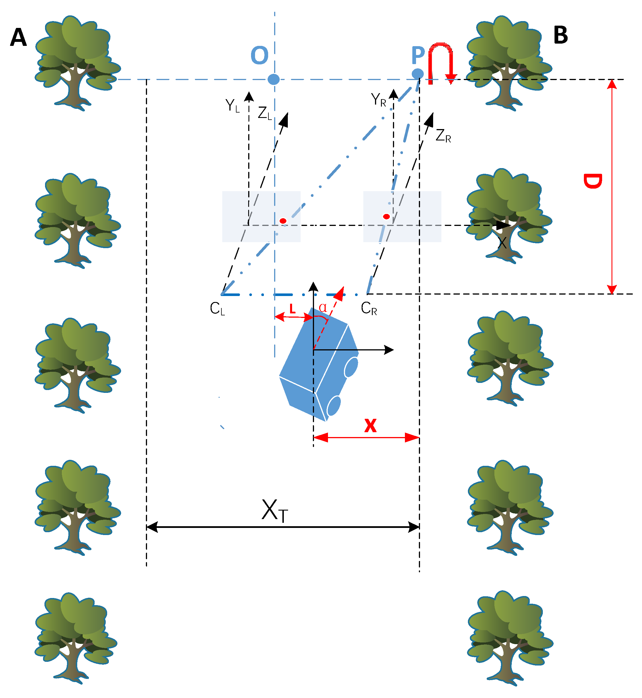
The principle of binocular vision depth perception is based on the human visual system, which uses the disparity between images observed by the left and right cameras to determine the distance of objects [25,26,27]. The process of recognizing steering markers by the orchard management robot in the orchard is shown in Figure 11. The robot starts to identify the steering markers when it approaches the end of the row and uses the parallax method to obtain the depth D and lateral distance X of the steering markers.

Due to the integration of the IMU (Inertial Measurement Unit) in the binocular camera, the attitude of the orchard management robot is adjusted before entering the inter-row operation. The longitudinal axis of the robot is aligned parallel to the centerline of the tree row. At this point, the IMU value is recorded as the baseline value k₁. During inter-row operation, the robot continuously collects IMU values, and the newly obtained value is denoted as k₂. The difference between k₂ and k₁ represents the heading angle α. In the diagram, the midpoint O of the line connecting the end trees A and B is considered as the steering start point for the robot. X_T represents the inter-row distance, L represents the lateral distance between the robot and the steering start point, and α represents the heading angle of the robot. When the robot reaches the end of the row, where D = 0, |L| ≤ 10 cm, and |α| ≤ 15°, it indicates that the robot is close to the steering start point. At this stage, the turning or U-turn can be initiated by calling the steering control function.

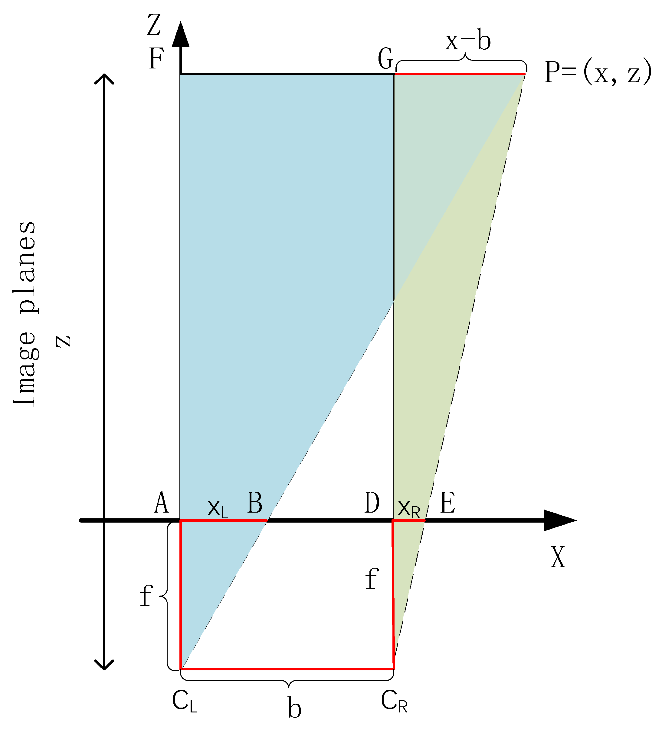
A bird’s-eye view of the binocular camera setup is shown in Figure 12, where the cameras are treated as pinhole cameras (horizontally placed), and the centers of the apertures of the two cameras are aligned on the x-axis. The distance between them is called the baseline (denoted as b) of the binocular camera. C_L and C_R represent the centers of the left and right apertures, respectively, the rectangle represents the image plane, and f represents the focal length. Consider a spatial point P, which has an image in each of the left-eye and right-eye cameras, denoted P_L, P_R. These 2 imaging positions differ due to the presence of the camera baseline. Ideally, since the left and right cameras deviate in position only on the x-axis, the image of point P also differs only on the x-axis P [28]. X_L and X_R are the left and right coordinates of the imaging plane, respectively.

According to the similarity principle between ΔABC_L and ΔFPC_L or ΔDEC_R and ΔGPC_R,

$$\frac{z}{f}=\frac{x}{x_L}\mathrm{or}\frac{z}{f}=\frac{x-\mathrm{b}}{x_R}$$

(10)

After converting Equation (10),

$$z=\frac{fb}{x_L-{\mathrm{x}}_R}=\frac{fb}{d}$$

(11)

$$d=x_L-x_R$$

(12)

Through Equations (10)–(12), the x and z coordinates of the target point can be calculated after obtaining the parallax d with the known baseline and focal length. The x coordinate is then the lateral distance of the steering mark (X), and the z coordinate is the depth of the steering mark (D). Finally, the lateral distance L between the robot and the steering start point can be obtained by Equations (13) and (14), which are calculated as follows:

When the steering start point is at the left front of the robot,

$$L=\frac{X_T}{2}-X$$

(13)

When the steering start point is at the right front of the robot,

$$L=X-\frac{X_T}{2}$$

(14)

The tool SDK accompanying the ZED2i binocular camera is used to obtain the pixel position information of the target area in combination with the OPENCV library and API. When the binocular camera acquires the image, the position of the steering marker in the image is obtained through the target detection algorithm; the depth and lateral distance of the pixel from the camera is obtained through the formula, and it is converted into the position information of the robot’s steering start point. Whether the robot reaches the steering start point or not is judged according to the information of the depth distance (D), the lateral distance (L), and the heading angle (α) between the robot and the steering start point.

3. Results and Analysis

3.1. Test Environment and Parameter Setting

The specific configuration of the deep learning environment for this study is shown in

Table 1. Training and test environment configuration table.

Configuration	Parameter
Operating System	Windows10
CPU	Intel Core i5-12400F CPU 4.4 GHz
GPU	GeForce RTX 1080Ti 11 G
Running Memory	16 G
Accelerate Environment	CUDA11.0 CuDNN7.6.5
Pytorch	1.7.1

.

For DFC-YOLOv7 network training, the parameters were set as follows: the number of samples for iterative training Batch size was 8, the number of iterations was set to 200 each time, the initial learning rate was 0.001, the momentum factor was 0.95, and, every 20 trainings, a training weight was saved, and the learning rate was reduced by a factor of 10. In the initial model training, using the “yolov7.pth”pre-training weights file, each subsequent training used the optimal weights generated from the previous training as the weights for this trial.

3.2. Evaluation Metrics for the Steering Mark Detection Test

In this study, average precision (AP), mean average precision (mAP), and single image detection speed were used as evaluation indexes. AP is related to the P (Precision) and R (Recall) of the model, and the formulas for calculating P, R, AP, and mAP are shown in Equations (15)–(18).

$$P=\frac{\mathrm{TP}}{\mathrm{TP}+\mathrm{FP}}\times 100\%$$

(15)

$$R=\frac{\mathrm{TP}}{\mathrm{TP}+\mathrm{FN}}\times 100\%$$

(16)

$$AP={\displaystyle \int {}_0^{1}P\left(R\right)\mathrm{d}R}$$

(17)

$$mAP=\frac{{\displaystyle \int {}_0^{1}P\left(R\right)\mathrm{d}}R}{N}$$

(18)

where TP is the number of correct model detections, FP is the number of model detection errors and target classification errors, FN is the number of model misses, and N is the number of categories. In this paper, the threshold was set to 0.5, and only when the IOU between the prediction box and the ground truth box exceeds 0.5, the prediction box was considered as a positive sample, otherwise it was a negative sample.

3.3. Steering Marker Positioning Test Evaluation Method

In this experiment, a steering marker localization test was conducted in an outdoor environment using a ZED2i binocular camera to verify the accuracy and stability of the localization method of the orchard management robot. Before the start of the experiment, in order to assess the accuracy of the ranging results, the depth of the steering mark from the camera (Z direction) as well as the lateral distance (X direction) were first measured using a laser rangefinder, which was taken as the true distance value.

After that, the ranging program is started to locate the steering mark, obtain the depth and lateral distance prediction of the steering mark position, and compare the prediction and the real value for analysis. The target distance information output from the positioning program was recorded. A total of nine ranging tests are conducted, and the error mean E_D is utilized as an evaluation index of positioning accuracy; the calculation formula is shown below:

$$E_D=\frac{{\displaystyle \sum _{i=1}^n\left|D_{\mathrm{d}i}-D_i\right|}}{n}$$

(19)

where D_di is the different measurements for the same position in each group of tests, and D_i is the true value of the distance for each group of tests. n is the number of groups.

3.4. Steering Marker Detection Model Training Results

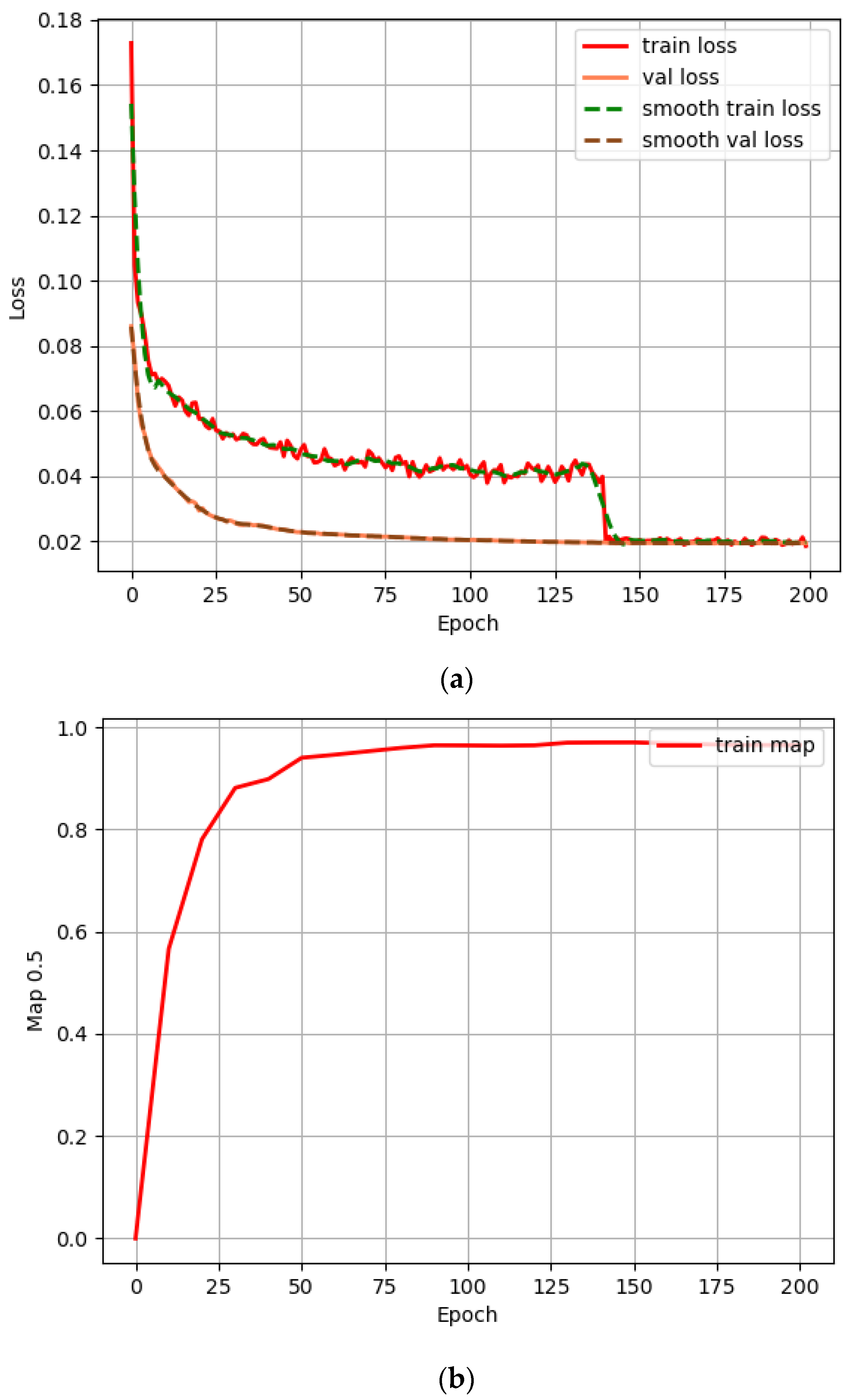
The DFC-YOLOv7 model was used for training and validation on the steering la-beling dataset. The loss function results generated from the training and validation sets during the last training are shown in Figure 13a.

As can be seen in Figure 13a, the DFC-YOLOv7 network model decreases the validation set loss value (val loss) and the training set loss value (train loss) with the increase in the number of iterations, and the mAP increases, as can be seen in Figure 13b. After 140 iterations, the training set loss value, the validation set loss value, and the mAP leveled off and the model converged. Due to the prior preprocessing of the dataset, the model tends to converge after fewer iterations, and the detection effect meets expectation.

3.5. Impact of Focal Loss Function on Multi-Class Task Models

In order to determine the effect of the attenuation parameter γ on the model when calculating the loss function, we drew the following conclusions in the yolo_train.py file by changing the parameter value of loss gamma in the dataset configuration file: (1) Regarding the model training loss, when γ = 0.5, there is a non-convergence phenomenon (the larger the value of γ the smaller the loss). (2) Regarding the mean accuracy mAP value, the mAP value of the model is improved when 1.0 ≤ γ ≤ 2.5. Based on this, four decay parameters—γ = 0.5, 1.0, 2.0, 2.5—were set, and the performance of the improved model was compared with that before the improvement (γ = 0), and the results obtained are shown in

Table 2. Comparison of the effects of attenuation parameters γ = 0.5, 1.0, 1.5 and γ = 0 on model performance.

Attenuation Parameters γ	AP/%				mAP/%
	A	B	C	D
0	94.45	91.23	96.65	95.15	94.37
0.5	93.21	91.4	95.88	96.2	94.17
1.0	94.8	91.4	97.01	96.4	94.90
2.0	95.2	92.7	96.9	96.69	95.37
2.5	95.02	91.98	96.73	96.42	95.04

Note: γ denotes the attenuation parameter. A denotes a left turn, B denotes a right turn, C denotes Turn left and make a U-turn, and D denotes Turn right and make a U-turn.

.

As shown in Table 2, when 1 ≤ γ ≤ 2.5, the loss function is more effective in improving the performance of the model. When γ = 2.0, the improved loss function improves the mAP value by 1.0% over the pre-improvement mAP value and improves the AP value of categories A and B by 0.75% and 1.47%, respectively, and it can be seen that the loss function strengthens the samples of the two categories A and B with a small number of samples so that the phenomenon of the low recognition rate caused by the sample imbalance can be improved.

3.6. Performance Comparison of Different Attention Mechanisms

In order to verify the advantages of the CBAM attention mechanism module used in this study, the CBAM attention mechanism module was replaced with the SE (squeeze-and-excitation) attention mechanism module and the ECA (efficient channel attention) attention mechanism module at the same locations in the network for separate experiments. The experimental results are shown in

Table 3. Performance comparison of the three attention mechanism modules.

Models	AP/%				mAP/%	Time/ms
	A	B	C	D
Base	95.2	92.7	96.9	96.69	95.37	15.21
SE-Base	94.45	91.23	96.65	95.15	94.37	15.44
ECA-Base	96.1	93.2	96.5	97.2	95.75	14.39
CBAM-Base	96.8	93.8	98.7	98.1	96.85	15.47

Note: Base represents the DFC-YOLOv7 model without incorporating the attention mechanism; Time denotes the single-image detection time. A denotes a left turn, B denotes a right turn, C denotes Turn left and make a U-turn, and D denotes Turn right and make a U-turn.

.

As shown in Table 3, after adding the different attention mechanism modules, all the indicators of the model changed; overall, the newer models demonstrated improvement over the original model. Among them, the DFC-YOLOv7 model with the addition of the CBAM attention mechanism module performed the best, with the mAP value improving by 1.48% compared to the DFC-YOLOv7 model without the integration of the attention mechanism, and this value improved by 2.48% and 1.1% compared to the model with the integration of the SE and ECA, respectively. This indicates that the CBAM attention mechanism is suitable for this study. The tandem connection of the two modules in CBAM better solves the problem of SE and ECA, which only focus on the channel information. CBAM gives more attention to steering markers by connecting the channel and spatial modules in tandem, which makes the model-extracted features point to the channel information attention, which makes the features extracted by the model more directional and more superior with respect to the steering marker identification task.

3.7. Ablation Experiment

The DFC-YOLOv7 algorithm makes several improvements over the original YOLOv7 algorithm. First, depth-separable convolution is introduced into the structure of the backbone feature extraction network and the reinforcement feature extraction network to replace some of the 3 × 3 ordinary convolution operations. Second, a Focal Loss function designed for multi-classification tasks is used to further improve the performance of the model in target detection. Finally, the CBAM Convolutional Attention Mechanism module is inserted after the three feature layers output from the backbone feature extraction network to enhance the model’s attention to important features. In order to more clearly analyze the improvement effect of the DFC-YOLOv7 algorithm on the original YOLOv7 algorithm, we conducted ablation experiments and designed eight sets of experiments, the results of which are shown in

Table 4. Results of ablation experiments.

Models	AP/%				MAP/%	Time/ms
	A	B	C	D
YOLOv7	94.45	91.23	96.65	95.15	94.37	24.96
DW-YOLOv7	94.32	91.33	96.7	95.61	94.49	13.48
Focal-YOLOv7	95.2	92.7	96.9	96.69	95.37	26.87
CBAM-YOLOv7	95.3	92.65	96.88	96.32	95.28	27.95
DF-YOLOv7	95.12	92.79	96.89	96.98	95.46	15.21
DC-YOLOv7	95.6	92.34	96.89	96.28	95.28	16.84
FC-YOLOv7	96.4	93.7	98.27	97.98	96.59	29.44
DFC-YOLOv7	96.8	93.8	98.7	98.1	96.85	15.47

Note: DW-YOLOv7 only uses DSC in the YOLOv7 algorithm; Focal-YOLOv7 only introduces the Focal loss function to the YOLOv7 algorithm; CBAM-YOLOv7 only introduces the CBAM attention mechanism to the YOLOv7 algorithm; DF-YOLOv7 uses DSC and the introduction of the Focal loss function; DC-YOLOv7 incorporates the use of DSC and the introduction of the CBAM attentional mechanism into the YOLOv7 algorithm; FC-YOLOv7 incorporates the introduction of the Focal loss function and CBAM attentional mechanism into the YOLOv7 algorithm; DCF-YOLOv7 incorporates the use of DSC, the introduction of the Focal loss function, and the introduction of CBAM attention mechanism.

. The results of these experiments demonstrate the impact and performance enhancement of the DFC-YOLOv7 algorithm in terms of different improvements.

As can be seen in Table 4, the detection time of a single image is reduced by 9.75 ms compared with the original model when replacing part of the ordinary 3 × 3 convolution using depth separable convolution, proving that the number of model parameters is reduced significantly. After the introduction of the Focal loss function, the accuracy of the A and B samples with a smaller number of samples is significantly improved, shortening the gap between the accuracy of different samples. After adding the CBAM attention mechanism module, the model’s attention to the detection target increases, and the accuracies of the four samples are improved; therefore, the simultaneous integration of these three methods in the YOLOv7 model can simultaneously take into account the detection accuracy and detection speed of the model, which achieves the desired goal.

3.8. Detection of Orchard Turning Mark by Different Models

The results of the steering labeling tests of the DFC-YOLOv7 model with other models on the validation set for different signs are shown in

Table 5. Training results of different models.

Models	AP/%				MAP/%	Time/ms
	A	B	C	D
YOLOv4	91.07	94.45	93.04	93.17	92.93	26.47
YOLOv4-tiny	90.86	81.26	92.07	92.89	89.27	6.86
YOLOv5-s	94.12	84.65	97.67	93.81	92.56	11.68
YOLOv7	94.45	91.23	96.65	95.15	94.37	24.96
DFC-YOLOv7	96.8	93.8	98.7	98.1	96.85	15.47

. From Table 5, it can be seen that the mAP value of the improved model is improved by 3.92%, 7.58%, 4.29%, and 2.48% compared to YOLOv4, YOLOv4-tiny, YOLOv5-s, and YOLOv7, respectively, but it is not as good as YOLOv4-tiny in terms of detecting speed; however, YOLOv4-tiny does not perform well in terms of detecting accuracy, and it can work phenomena such as wrong detection and missed detection, which affects the normal work of the orchard management robot. Therefore, after comparison, we found that the DFC-YOLOv7 model has a better overall performance in terms of detection speed and detection accuracy, which can satisfy our expected goals and realize the fast and accurate detection of orchard turning marks for the orchard management robot.

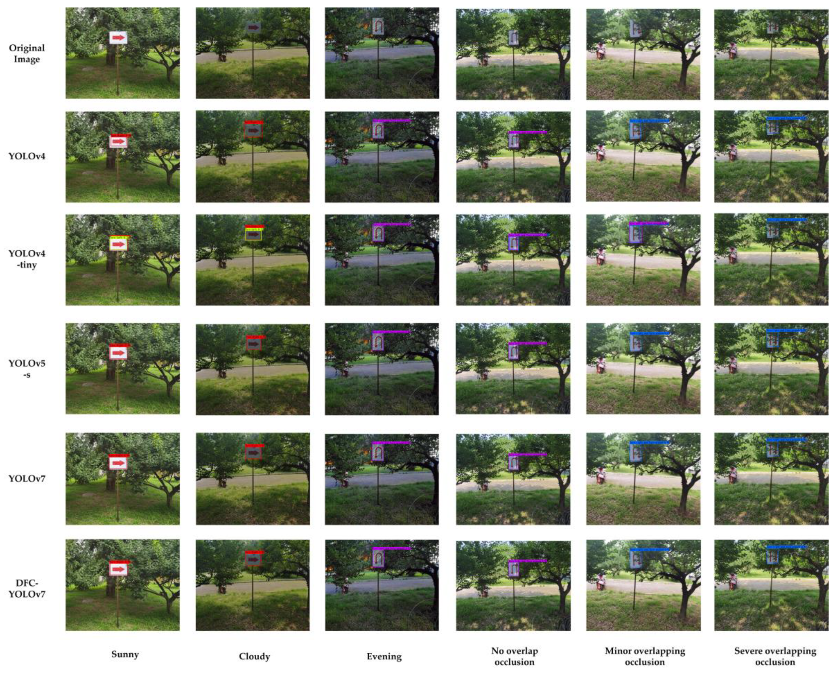
In order to test the performance of different trained models in detecting signage under different conditions, we took 300 new photos in the orchard for testing purposes, which were categorized into six scenarios, namely, sunny, cloudy, evening, no overlapping occlusion, slight overlapping occlusion, and severe overlapping occlusion, and the results of their detection are shown in Figure 14. From the figure, it can be seen that, in the cases of cloudy weather, evening weather, and severe occlusion, except for the DFC-YOLOv7 model, the correctness values of all the other models are affected, which is because, in the case of bad lighting and occlusion, the steering arrow features of the steering markers are not obvious enough; therefore, the model can not accurately extract their features. Among them, YOLOv4-tiny had a misdetection due to its low detection accuracy, recognizing the right-turning signage as both right and left, which proved that the model was unable to distinguish the steering direction of the orchard management robot. Therefore, compared with other models, the DFC-YOLOv7 model is insensitive to light changes and can provide accurate steering information for the robot when it is working around the clock, greatly avoiding misdetection and the omission of detection (problems that exist in other models).

3.9. Binocular Camera Localization Results

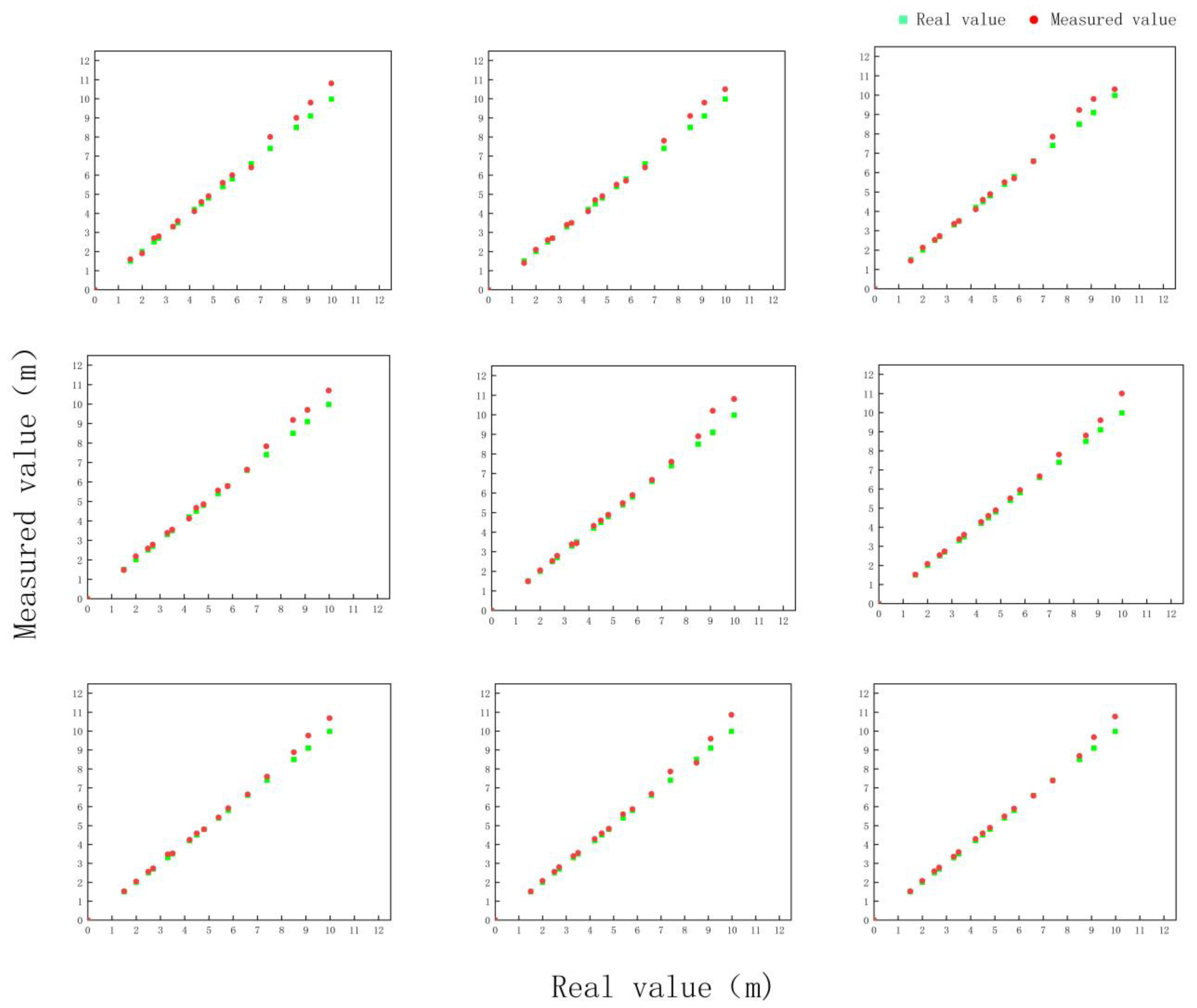
The comparison results between the distance measurement data obtained from the steering marker depth test and the true data are shown in Figure 15. The results indicate that there is a larger overlap between the measured values and the true values at close distances, while the overlap is smaller at far distances during the process of the orchard management robot approaching the steering markers. Therefore, the measured values of depth D and lateral distance X obtained by the robot when approaching the steering markers are relatively accurate.

In addition, fitting and comparing the experimental data from nine repeated tests yields Figure 16a. From this figure, it can be observed that under different test conditions, there is a larger degree of data dispersion at far distances compared to close distances. Furthermore, by calculating the maximum and minimum deviations of each dataset from the true data, as shown in Figure 16b, an average error of 0.046 m was obtained for the nine test sets when the distance was less than 5 m. Therefore, when the orchard management robot approaches the steering markers, the binocular camera can accurately measure the depth D and lateral distance X of the steering markers. These two pieces of information are then converted into the depth D and lateral distance L between the robot and the starting point of the steering, enabling the localization of the starting point. This ensures that the robot makes timely steering adjustments, reducing steering time and improving work efficiency.

4. Discussion

In this paper, we proposed an improved DFC-YOLOv7 target detection algorithm for steering labeling detection to guide an orchard management robot for autonomous steering in a complex orchard environment. Based on the original YOLOv7 model, we replaced some 3 × 3 ordinary convolutions with depth-separable convolutions and introduced the Focal loss function as well as the CBAM attention mechanism. This ensures the detection speed and improves the detection accuracy of the model. At the same time, we utilized a binocular camera to obtain the depth D, lateral distance L, and heading angle α of the orchard robot with respect to the steering start point. This information provides the initial positional information for the autonomous steering of the robot, which ensures that the robot is able to carry out the autonomous steering in time, thus improving the robot’s work efficiency.

(1) The method achieves a mAP value of 96.85% under the validation set, and the detection time of a single image reaches 15.47 ms; compared with the other models, the mAP value of the improved model is 2.48% higher than that of the original model and 3.92%, 7.58%, and 4.29% higher than the YOLOv4, YOLOv4-tiny, and YOLOv5-s models, respectively. Meanwhile, the detection time of the improved model is shortened by 9.49 ms compared with the original model, indicating that the number of parameters of the DFC-YOLOv7 model is greatly reduced, which ensures both the detection accuracy and detection speed.

(2) In order to verify the detection effect of the model in real orchards, this model and other models were tested in different scenarios. The results show that, except for the DFC-YOLOv7 model, the correctness of the other models is affected, which is due to the fact that the steering arrow feature of the steering markers is not obvious enough for the model to accurately extract its features under poor illumination and occlusion. The DFC-YOLOv7 model is insensitive to illumination changes, and it can provide accurate steering direction information to the robot’s orchard ground while the robot is working.

(3) The binocular camera is used to obtain the depth D, lateral distance L, and heading angle α of the orchard robot relative to the steering start point. When the depth distance is less than 5 m, the mean value of the error of the nine groups of tests is 0.046 m, and the degree of dispersion regarding the data is larger when the depth distance is more than 7 m. Therefore, when the orchard management robot is close to the steering start point, the binocular camera can measure the more accurate attitude information of the steering start point, and when the orchard management robot reaches the steering start point, the robot starts to steer autonomously, and this method can avoid the problem of providing untimely steering to the orchard management robot.

References

1. Liu, F.; Wang, H.; Li, L. Status quo, problems and development countermeasures of China’s facility fruit tree industry. China Fruit Tree 2021, 217, 1–4. [Google Scholar]
2. Barbara, A.; Łukasz, P.; Solomiia, K. Pioneering Metabolomic Studies on Diaporthe eres Species Complex from Fruit Trees in the South-Eastern Poland. Molecules 2023, 28, 1175. [Google Scholar]
3. Sayyad-Amin, P. A Review on Breeding Fruit Trees Against Climate Changes. Erwerbs-Obstbau 2022, 64, 697–701. [Google Scholar] [CrossRef]
4. Satyam, R.; Jens, F.; Thomas, H. Navigation and control development for a four-wheel-steered mobile orchard robot using model-based design. Comput. Electron. Agric. 2022, 202, 107410. [Google Scholar]
5. Xing, W.; Han, W.; Hong, Y. Geometry-aware fruit grasping estimation for robotic harvesting in apple orchards. Comput. Electron. Agric. 2022, 193, 106716. [Google Scholar]
6. Bell, J.; MacDonald, A.; Ahn, S. An Analysis of Automated Guided Vehicle Standards to Inform the Development of Mobile Orchard Robots. IFAC Pap. 2016, 49, 475–480. [Google Scholar] [CrossRef]
7. Zhang, S. Research on Autonomous Obstacle Avoidance Motion Planning Method for Mobile Robots in Orchard. Master’s Thesis, Jiangsu University, Zhenjiang, China, 2022. [Google Scholar]
8. Zhen, N.; Yi, D.; Qing, Y. Dynamic path planning method for headland turning of unmanned agricultural vehicles. Comput. Electron. Agric. 2023, 206, 107699. [Google Scholar]
9. Qian, R.; Zhang, B.; Yue, Y. Traffic sign detection by template matching based on multilevel chain code histogram. In Proceedings of the 12th International Conference on Fuzzy Systems and Knowledge Discovery (FSKD), Zhangjiajie, China, 15–17 August 2015; IEEE: Piscataway, NJ, USA, 2015; pp. 2400–2404. [Google Scholar]
10. Liang, M.; Yuan, M.; Hu, X. Traffic sign detection by ROI extraction and histogram features-based recognition. In Proceedings of the 2013 International Joint Conference on Neural Networks (IJCNN), Dallas, TX, USA, 4–9 August 2013; IEEE: Piscataway, NJ, USA, 2013; pp. 1–8. [Google Scholar]
11. Chen, Z.; Li, L.; Li, Z. Research on license plate recognition technology based on machine learning. Comput. Technol. Dev. 2020, 30, 13–18. [Google Scholar]
12. Jiang, L.; Chai, X.; Li, L. Positioning study of contact network column signage between rail zones. Intell. Comput. Appl. 2020, 10, 154–157+160. [Google Scholar]
13. Zhou, F.; Jin, L.; Dong, J. A review of convolutional neural network research. J. Comput. 2017, 40, 1229–1251. [Google Scholar]
14. Jordan, M.; Mitchell, T. Machine learning: Trends, perspectives, and prospects. Science 2015, 349, 255–260. [Google Scholar] [CrossRef]
15. Schmidhuber, J. Deep learning in neural networks: An overview. Neural Netw. 2015, 61, 85–117. [Google Scholar] [CrossRef]
16. Liang, W.; Ling, M.; Hao, W. Real-time vehicle identification and tracking during agricultural master-slave follow-up operation using improved YOLO v4 and binocular positioning. Proc. Inst. Mech. Eng. Part C J. Mech. Eng. Sci. 2023, 237, 1393–1404. [Google Scholar]
17. Matko, G.; Nikola, A.; Ivan, L. Detection and Classification of Printed Circuit Boards Using YOLO Algorithm. Electronics 2023, 12, 667. [Google Scholar]
18. Tai, H.; Si, Y.; Qi, M. Lightweight tomato real-time detection method based on improved YOLO and mobile deployment. Comput. Electron. Agric. 2023, 205, 107625. [Google Scholar]
19. Wang, C.; Bochkovskiy, A.; Liao, H. YOLOv7: Trainable bag-of-freebies sets new state-of-the-art for real-time object detectors. arXiv 2022, arXiv:2207.02696. [Google Scholar]
20. Zhi, J.; Jin, F.; Jie, Z. An efficient SMD-PCBA detection based on YOLOv7 network model. Eng. Appl. Artif. Intell. 2023, 124, 106492. [Google Scholar]
21. Zi, Y.; Aohua, S.; Si, Y. DSC-HRNet: A lightweight teaching pose estimation model with depthwise separable convolution and deep high-resolution representation learning in computer-aided education. Int. J. Inf. Technol. 2023, 15, 2373–2385. [Google Scholar]
22. Emin, M. Hyperspectral image classification method based on squeeze-and-excitation networks, depthwise separable convolution and multibranch feature fusion. Earth Sci. Inform. 2023, 16, 1427–1448. [Google Scholar]
23. Lin, T.; Goyal, P.; Girshick, R. Focal loss for dense object detection. In Proceedings of the IEEE International Conference on Computer Vision, Venice, Italy, 22–29 October 2017; pp. 2980–2988. [Google Scholar]
24. Woo, S.; Park, J.; Lee, J. Cbam: Convolutional block attention module. In Proceedings of the European Conference on Computer Vision (ECCV), Munich, Germany, 8–14 September 2018; pp. 3–19. [Google Scholar]
25. Auria, E.; Nairouz, F.; Uri, P. Temporal synchronization elicits enhancement of binocular vision functions. iScience 2023, 26, 105960. [Google Scholar]
26. Yiping, S.; Zheng, S.; Bao, C. A Point Cloud Data-Driven Pallet Pose Estimation Method Using an Active Binocular Vision Sensor. Sensors 2023, 23, 1217. [Google Scholar]
27. Shi, X.; Jiang, W.; Zheng, Z. Bolt loosening angle detection based on binocular vision. Meas. Sci. Technol. 2023, 34, 035401. [Google Scholar]
28. Jia, K.; Peng, S.; Zhi, J. Research on a Real-Time Monitoring Method for the Three-Dimensional Straightness of a Scraper Conveyor Based on Binocular Vision. Mathematics 2022, 10, 3545. [Google Scholar]
Figure 1. Four different signs for the four steering markers.
Electronics 12 03614 g001
Figure 2. Roadmap of the orchard management robot in action.
Electronics 12 03614 g002
Figure 3. Steering marker images for complex scenes.
Electronics 12 03614 g003
Figure 4. (a) Mixup data enhancement effect; (b) type and number of labels in the training set.
Electronics 12 03614 g004
Figure 5. Mosaic data enhancement.
Electronics 12 03614 g005
Figure 6. Two different kinds of convolutional structures.
Electronics 12 03614 g006
Figure 7. Structure diagram of CBAM. CAM denotes Channel Attention Mechanism Module; SAM denotes Spatial Attention Mechanism Module.
Electronics 12 03614 g007
Figure 8. Structure diagram of CAM. GAM represents the Global Max Pooling; GAP represents the Global Average Pooling. The shared MLP is composed of a multi-layer perceptron with one hidden layer.
Electronics 12 03614 g008
Figure 9. Structure diagram of SAM. GAM represents the Global Max Pooling; GAP represents the Global Average Pooling.
Electronics 12 03614 g009
Figure 10. DFC-YOLOv7 network structure model. CBS is Conv + BN + SILU; DBS is DSC + BN + SILU. Conv denotes ordinary convolution; DSC denotes depth separable convolution; BN denotes bulk regularization; SILU denotes activation function. E-ELAN denotes extended efficient layer aggregation networks; MP represents Maxpool (Maximum Pooling) + DBS; CBAM represents the Convolutional Block Attention Module; SPPCSPC represents Spatial Pyramid Pooling Structure; UPSample represents the upsampling; Concat and Cat represent Feature Connectivity; RepCon represents Reparameterization Convolution; the Head is the prediction head.
Electronics 12 03614 g010
Figure 11. The orchard management robot recognizes the steering marking process in the orchard. A and B represent the fruit trees at the end of the row. D is the depth distance between the robot and the marker. X is the lateral distance between the robot and the marker. O is the start point of the robot’s turn. P is the center of the marker. L represents the lateral distance between the robot and the steering start point. α represents the robot’s heading angle. Red dot represents the imaging point of the marker on the binocular camera. XT represents the distance between rows of fruit trees. CL and CR represent the centers of the left and right apertures.
Electronics 12 03614 g011
Figure 12. A bird’s-eye view of the binocular camera operation. CL and CR represent the centers of the left and right apertures. f is the focal length of the camera. XL and XR are the left and right coordinates of the imaging plane, respectively. Blue triangles and green triangles represent the imaging planes of the left and right cameras, respectively.
Electronics 12 03614 g012
Figure 13. (a) Loss curves; (b) mAP curves.
Electronics 12 03614 g013
Figure 14. Detection of steering markers by different models in different scenarios.
Electronics 12 03614 g014
Figure 15. Comparison of true and measured values of the steering mark depth test.
Electronics 12 03614 g015
Figure 16. (a) Fitting curve of measured values; (b) Error curve of true values and measured values.
Electronics 12 03614 g016