CANARY: An Adversarial Robustness Evaluation Platform for Deep Learning Models on Image Classification

Abstract

The vulnerability of deep-learning-based image classification models to erroneous conclusions in the presence of small perturbations crafted by attackers has prompted attention to the question of the models’ robustness level. However, the question of how to comprehensively and fairly measure the adversarial robustness of models with different structures and defenses as well as the performance of different attack methods has never been accurately answered. In this work, we present the design, implementation, and evaluation of Canary, a platform that aims to answer this question. Canary uses a common scoring framework that includes 4 dimensions with 26 (sub)metrics for evaluation. First, Canary generates and selects valid adversarial examples and collects metrics data through a series of tests. Then it uses a two-way evaluation strategy to guide the data organization and finally integrates all the data to give the scores for model robustness and attack effectiveness. In this process, we use Item Response Theory (IRT) for the first time to ensure that all the metrics can be fairly calculated into a score that can visually measure the capability. In order to fully demonstrate the effectiveness of Canary, we conducted large-scale testing of 15 representative models trained on the ImageNet dataset using 12 white-box attacks and 12 black-box attacks and came up with a series of in-depth and interesting findings. This further illustrates the capabilities and strengths of Canary as a benchmarking platform. Our paper provides an open-source framework for model robustness evaluation, allowing researchers to perform comprehensive and rapid evaluations of models or attack/defense algorithms, thus inspiring further improvements and greatly benefiting future work.

1. Introduction

Nowadays, deep learning is widely used in image classification tasks and plays an irreplaceable role in security-sensitive areas such as autonomous driving [1], medical diagnosis [2,3,4], software security [5], and military reconnaissance [6]. However, small perturbations crafted by attackers can disturb image classification models to produce erroneous inference results [7]. It has been pointed out that there is an “arms race” between attack [8,9,10] and defense [11,12,13]. With a large number of means of attacks and defenses being proposed, how to fully and fairly measure the adversarial robustness of models with different structures and defense methods as well as the performance, strengths, and weaknesses of different attack methods has always been a challenge for researchers.

In order to comprehensively evaluate the security of deep learning models, some research [14,15,16,17,18,19,20,21,22] has proposed evaluation metrics, method libraries, and evaluation platforms. Works such as CleverHans [14] and FoolBox [15] integrated the most common attack and defense methods, but the neglect of code quality made some of them incorrectly developed or even unworkable. DeepSec [18] first proposed a series of evaluation metrics for both attack and defense methods but needed to exhaustively validate the effectiveness of these metrics and set a baseline and rank these methods based on the metrics. RealSafe [20] abandoned these metrics and instead used two complementary robustness curves as the primary evaluation metrics, focusing on the misclassification rate of attacks under different perturbation budgets. In fact, the evaluation strategy of RealSafe did not always work for attacks that limit the reduction of the misclassification rate while optimizing perturbations (e.g., Boundary Attack) or for attacks that are difficult to precisely limit the scale of perturbations (e.g., CW [23]). AISafety [22] attempted to extend the work of both. However, it neglected the universality of the evaluation metrics, and its interpretability and neuron traversal evaluation were difficult to widely adapt to models with different structures. Furthermore, almost all work evaluated only a few models (e.g., RealSafe only evaluated ResNet [24] and Inception, while DeepSec only evaluated ResNet, and AISafety only evaluated VGG [25] and WRN [26]), which left us with a lack of knowledge on the performance of attack and defense methods on models with different structures. The evaluation frameworks proposed by these works also lacked sufficient flexibility and universality in the face of new methods, thus limiting their further role.

We note that evaluation metrics are still dominated by the misclassification rate and norm metrics, even in the latest work on adversarial methods. Researchers drew different conclusions based on different models and different parameters and claimed that their findings were in a sense the best (we have already revealed that attack methods can perform very differently on different models, see Section 5.5 for further discussion). Clearly, the results of such evaluations may be biased, and incomplete evaluations could not provide them with convincing conclusions.

In this work, hoping to facilitate future research, we develop a comprehensive, generic scoring framework of 26 (sub)metrics to evaluate the adversarial robustness of models. First, we define a valid example selection strategy that avoids iterative testing of different perturbations, allows for faster conclusions than RealSafe, and can be adapted to a wider range of attack methods. Second, we propose a two-way evaluation strategy of “Attack Effectiveness–Model Robustness”, which allows us to fully understand the performance of existing attacks on different models and the robustness of existing models in the face of different attacks. We finally propose a novel integrated capability measure based on Item Response Theory (IRT [27]) for the first time, which can adequately measure the difficulty and differentiation of metrics based on Markov Chain Monte Carlo (MCMC [28]), and can give an “Attack Effectiveness–Model Robustness” capability score for attacks and models.

We integrate a large number of classical and SOTA attacks for bi-directional evaluation, including 12 white-box attacks and 12 black-box attacks. These attacks cover the widest range of attack paths, attack means, and distance measures, including (1) gradient-based attacks, transfer-based attacks, score-based attacks, and decision-based attacks; (2) frequency-domain- and time-domain-based attacks; and (3) attacks based on $L_0,L_2,L_{\infty }$. To fully demonstrate the differences in robustness between models with different structures, we selected the 15 most representative models ranging from AlexNet [29] to ConvNeXt [30] in the evaluation. We conducted large-scale experiments with these models and methods on the ImageNet [31] dataset. Using quantitative results, we show the differences in misclassification and imperceptibility capabilities between different attack methods and further analyze the competition between them; we also show the differences in the robustness of the different structural models and, furthermore, which attack methods work better or worse against which models. We also provide a more intuitive capability score to help researchers understand the robustness of different models and the differences in the effectiveness of different attack methods more clearly.

We developed a new adversarial robustness evaluation platform, Canary, on which we have based all our evaluation experiments. The structure is shown in Figure 1. We hope to open-source the platform, share all our evaluation data, and continue to integrate more attack and defense methods. We hope that more researchers will evaluate their work in the platform in order to provide a reliable benchmark, which we believe can help fellow researchers to better understand adversarial attacks and further improve the robustness of their models.

Our contributions can be summarized as follows:

• We propose novel evaluation methods for model robustness, attack/defense effectiveness, and attack transferability and develop a scoring framework including 26 (sub)metrics. We first use IRT to calculate these metrics into scores that reflect their real capabilities, making it possible for us to compare and rank model robustness and the effectiveness of the attack method.
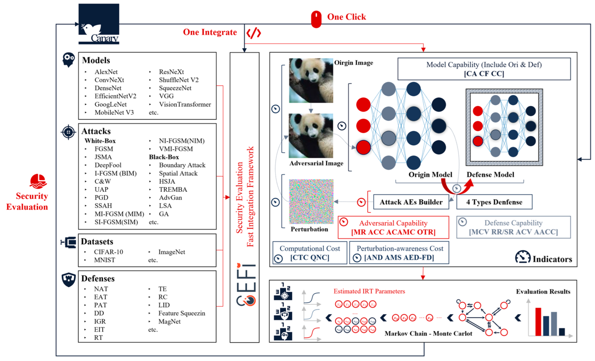
• We design and open-source an advanced evaluation platform called Canary, including 17K lines of code. The platform contains at least 30 attacks, including 15 white-box attacks and 15 black-box attacks. To our knowledge, this is one of the best platforms that can allow users to freely integrate any CNN model or any attack or defense method.
• Based on Canary and the scoring framework, we conducted the largest-scale cross-evaluation experiment of “model-attack” to date and obtained a series of interesting and insightful findings. In particular, we revealed the significantly different performances of different models under the same attack and the substantial differences of different attack methods in attacking the same model. These findings may promote the development of the adversarial learning field.
• We have collated the test results into a database and open-sourced it with a view to providing a valid baseline for other researchers, which will be the second baseline for model robustness since RobustBench.

Notations

For ease of understanding, we summarize the basic notations used in this paper in

Table 1. Base notations used in this paper.

Notations	Description
$x=\left\{x_1,\cdots ,x_n\right\}$	$x$ is the set of $n$ original images, where $x_i$ denotes the $i$th image in the set.
$y=\left\{y_1,\cdots ,y_n\right\}$	$y$ is the set of $n$ original images corresponding to ground-truth labels, where $y_i$ denotes the label of the $i$th image in the set $x$, and $y_i\in \left\{1,\cdots ,k\right\}$.
$F:x_i\to y_i^{*}$,${ y}_i^{*}\in \left\{1,\cdots ,k\right\}$	$F$ is a deep-learning-based image k-class classifier that has $F\left(x_i\right)=y_i$ when classified correctly.
$P: x_i\to \left\{P\left(1\right),\cdots ,P\left(k\right)\right\}$	$P$ is the Softmax layer of $F$, $F\left(x_i\right)=\arg \underset{j}{\mathrm{m}\mathrm{a}\mathrm{x}} P{\left(x_i\right)}_j$.
$P{\left(x_i\right)}_j$	$P{\left(x_i\right)}_j$ denotes the probability that $x_i$ is inferred to be $j$ by $F$, also known as the confidence level, where $j\in \left\{1,\cdots ,k\right\}$.
$x^a$	$x^a$ is the adversarial example, where $x$ is generated by the attack method.
$y^{adv}$	For targeted attacks only, $y^{adv}$ is the label of the specified target.

, and any notation mentioned in the table will not be subject to additional explanation.

2. Related Works

In this section, we will provide a brief overview of existing works on adversarial attacks and defenses and those on adversarial robustness evaluation.

2.1. Methods of Adversarial Attack and Defense

Formally, an adversarial example can be defined as follows: Given an original image $x$ (where $x\in {\mathbb{R}}^{w\times h\times c}$, $w$ and $h$ are the dimensions of the image and $c$ is the number of its channels) and $F$ is a classification model trained from a set of clean images, then $F\left(x\right)$ is the inference of the original image $x$. If the perturbation $\delta \left(x\right)$ required to make $x$ cross the decision boundary of $F$ can be found such that $x^a=x+\delta \left(x\right)$ and $F\left(x\right)\ne F\left(x^a\right)$, then the image $x^a$ can be an adversarial example of $F$. Carlini and Wagner argue that the optimal adversarial example generation algorithm needs to ensure the following two conditions: (1) $\delta \left(x\right)$ is as small as possible (usually $\delta \left(x\right)$ uses $l_P$-norm, $p\in \left\{1,2,\infty \right\}$ to measure), while being as imperceptible to the human eye as possible; and (2) $x^a$ should be as effective as possible to make the $F$ classification produce errors [23]. For target attacks, the confidence level in the errors should also be sufficiently high.

Considering the attacker’s knowledge of the target model, it can be classified as either (1) a white-box attack or (2) a black-box attack. For white-box attacks, the attacker has full access to the model, can obtain the model structure, and can often obtain a high misclassification rate at a small perturbation cost, which is often used to evaluate the effectiveness of defense methods or the robustness of the model under adverse conditions. The most common white-box attacks are generally based on gradients to optimize perturbations and generate adversarial examples. For black-box attacks, the attacker only has access to the input and output information of the model but not its structure, and the main implementation methods are transfer-based and query-based attacks.

Query-based attacks rely on the model inference scores, increasing the misclassification rate at the cost of high accesses. Depending on the amount of information obtained, they can be further divided into decision-based attacks, which can only obtain hard-label, and score-based attacks, which can obtain a continuous inference score (i.e., the confidence level for each classification, soft-label). We have summarized many important adversarial attack algorithms based on the above definitions and descriptions. For more details see Appendix A: Details of the main adversarial attack algorithms in our evaluations.

The defense methods can be broadly classified into three categories: adversarial training, image processing, and adversarial example detection. For adversarial training, we consider the defended model $F_D$ to have a similar structure to the original model $F_O$ but with differences in the weight hyperparameters; for image processing, we consider $F_D\left(x\right)=F_O\left(\phi \right(x\left)\right)$, where $\phi$ is the image processing method; and for adversarial example detection, there is generally no modification to the model itself.

In this paper, we evaluate the following attack methods, shown in

Table 2. Main adversarial attack algorithms in computer vision in our experiment.

Algorithm	Perturbation Measurement	Attacker’s Knowledge		Attack Approach
FGSM [32]	$L_{\infty }$	white-box		gradient
JSMA [33]	$L_0$	white-box		gradient
DeepFool [34]	$L_0,L_2,L_{\infty }$	white-box		gradient
I-FGSM (BIM) [35]	$L_{\infty }$	white-box		gradient
C&W Attack [23]	$L_0,L_2,L_{\infty }$	white-box		gradient
Projected Gradient Descent (PGD) [36]	$L_1,L_{\infty }$	white-box		gradient
MI-FGSM (MIM) [37]	$L_{\infty }$	transferable black-box		transfer, gradient
SI-FGSM (SIM) [38]	$L_{\infty }$	transferable black-box		transfer, gradient
NI-FGSM (NIM) [38]	$L_{\infty }$	transferable black-box		transfer, gradient
VMI-FGSM (VMIM) [39]	$L_{\infty }$	transferable black-box		transfer, gradient
Elastic-Net Attack (EAD) [40]	$L_1$	white-box		gradient
SSAH [41]	-	white-box		gradient
One-pixel Attack (OPA) [42]	$L_0$	black-box	query, score	Soft Label
Local Search Attack (LSA) [43]	$L_0$	black-box	query, score	Soft-Label
Boundary Attack (BA) [44]	$L_2$	black-box	query, decision	Hard-Label
Spatial Attack (SA) [45]	-	black-box	query	Hard-Label
Hop Skip Jump Attack (HSJA) [46]	$L_2,L_{\infty }$	black-box	query, decision	Hard-Label
Gen Attack (GA) [47]	$L_2,L_{\infty }$	black-box	query, score	Soft-Label
SPSA [48]	$L_{\infty }$	black-box	query, score	Soft-Label
Zeroth-Order Optimization (ZOO) [49]	$L_2$	black-box	query, score	Soft-Label
AdvGan [50]	$L_2$	black-box	query, score	Soft-Label
TREMBA [51]	-	black-box	query, score	Soft-Label

.

2.2. The Robustness Evaluation of DL Model

Many different evaluation frameworks have been proposed to evaluate DL-model security comprehensively. These efforts can be broadly classified into three categories, namely the attack/defense toolsets represented by CleverHans [14], FoolBox [15], and ART [16]; the benchmarking methods/platforms represented by RealSafe [20] (upgraded version is Ares) and DEEPSEC [18]; and the evaluation database represented by RobustBench [21].

CleverHans is the first proposed library of DL-model attack and defense methods. Similarly, FoolBox and ART provide additional attack and defense methods and support running on various DL learning frameworks. Unfortunately, CleverHans has suspended updating maintenance and support since 2021 and has significantly fewer methods than the other method libraries. Attack method libraries such as FoolBox rely on community contributions and lack the necessary checks in late version iterations, leaving the correctness of the code open to question and controversy. These studies mainly focused on building open-source libraries for adversarial attacks and defenses and did not provide a comprehensive strategy for evaluating the security of DL models.

DEEPSEC provides a unified platform for adversarial robustness analysis of DL models, containing 16 attack methods and 10 attack-effectiveness metrics, 13 defense methods, and 5 defense-effectiveness metrics. Similarly, RealSafe and AISafety [22] add additional evaluation metrics to those described in DEEPSEC and update the attack and defense methods. However, while AISafety provides a variety of interpretable, neuronal coverage-related evaluation metrics, it relies heavily on specific attack methods and models and is difficult to apply to other models. Similarly, DEEPSEC provides a variety of attack and defense methods, but adding new attack/defense methods and models is relatively difficult, which makes it difficult to adapt to the latest attack/defense methods. To our knowledge, all such platforms do not analyze the evaluation metrics for level of difficulty and differentiation, nor do they provide a widely recognized ranking of the final evaluation results. While these studies provide evaluation methods and implementations, they still need to improve in terms of universality, ease of use, and interpretation of results.

RobustBench provides a widely recognized benchmark for evaluating the robustness of DL models. RobustBench uses the AutoAttack [52] attack method to evaluate and rank the security of multiple DL models trained on CIFAR-10. However, whether RobustBench can be used as a robustness evaluation metric that can be generalized to practical applications is still questioned by researchers. The RobustBench evaluation of model robustness is only tested by a single attack method, AutoAttack, which severely weakens the credibility and applicability of the evaluation results. Lorenz et al. proposed that detecting adversarial perturbations generated by the AutoAttack method itself is relatively easy, and other attack methods are better at concealment under the same misclassification rate. Also, the resolution of the CIFAR-10 dataset is too low, making it unable to be well generalized to higher-resolution images [53].

In terms of universality, the test metrics proposed by many test platforms impose harsh requirements on the structure of the models to be tested, making it difficult to be widely used; moreover, many attack libraries contain attack or defense algorithms that are limited by various conditions, making them difficult to adapt to all deep learning models; furthermore, due to the possible inability to find pre-defined execution logic, existing test platforms and some method libraries also have serious difficulties in integrating new models or attack and defense methods.

In terms of validity, many test platforms chose adversarial evaluation metrics that later proved ineffective or outdated. For example, the Neuron Coverage series of metrics were first used in DeepGauge [54] and integrated into frameworks such as AISafety. However, experiments by Yan et al. on these frameworks demonstrated the very limited correlation between these metrics and the security and robustness of neural networks [55].

In terms of completeness, there is a lack of correlation between different test platforms and method libraries, which makes them cover only a small number of attack and defense methods as well as a lack of different cross-tests and comparative tests. To our knowledge, apart from a few database platforms, such as RobustBench, other platforms do not yet provide benchmark evaluation databases and lack the necessary baselines for measurement. Furthermore, due to the lack of corresponding strategies, the evaluation results are also mostly a simple list of metrics and do not lead to conclusions worthy of attention.

In this paper, we replicate and evaluate the following models: AlexNet [29], VGG [25], GoogLeNet [56], InceptionV3 [57], ResNet [24], DenseNet [58], SqueezeNet [59], MobileNetV3 [60], ShuffleNetV2 [61], MNASNet [62], EfficientNetV2 [63], VisionTransformer (ViT) [64], RegNet [65], SwinTransformer (SwinT) [66], and ConvNeXt [30]. All of the above 15 models have a wide range of applications.

3. Measurement Metrics and Evaluation Methods

In order to effectively measure model security and the effectiveness of the attack and defense algorithms known to date, we have developed a universal, valid, and interpretable framework for evaluating the robustness of models and the effectiveness of attack and defense algorithms, which contains a total of 26 evaluation metrics (with sub-metrics) that can be widely used. A Python framework that has implemented all the evaluation metrics is also provided for researchers to use in their studies (see Section 4). In this section, we introduce our evaluation metrics framework and evaluation methodology while describing how these metrics can be used in combination to measure model robustness and attack/defense capabilities.

3.1. Measurement Metrics

The metrics framework we have designed for evaluation can be broadly divided into four parts: Model Capability Oriented, Adversarial Effect Oriented, Adversarial Cost Oriented, and Defense Effect Oriented. In this section, we will provide a detailed explanation of the rationale for selecting the metrics and their definitions and expressions.

3.1.1. Model Capability Measurement Metrics

We know that adversarial reinforcement learning generally improves the generalization of models to make them more robust against adversarial examples, but the inferential capability of the models may be negatively affected by this. It is, therefore, necessary to consider the models’ performance when ranking their overall ability and to give higher scores to models that perform better and are safer. In addition to this, the models themselves need to be taken into account when trying to compare attack or defense methods tested on different models. We consider the following measurement metrics:

Clean Example Accuracy (Clear Accuracy, CA): The accuracy of the model for the classification of the clean dataset. CA can be expressed as:

$$\mathrm{C}\mathrm{A}=\frac{1}{n}{\mathsf{\Sigma }}_{i=1}^{n}count\left(F\left(x_i\right)=y_i\right)$$

(1)

Clean Example F1 score (Clear F1, CF): The F1 score of the model for classification of the clean dataset. Let ${TP}_i={\mathsf{\Sigma }}_{k=1}^{n}count\left(F\left(x_i\right)=y_k,y_i=y_k\right)$; ${FP}_i={\mathsf{\Sigma }}_{k=1}^{n}count\left(F\left(x_i\right)=y_k,y_i\ne y_k\right)$; ${FN}_i={\mathsf{\Sigma }}_{k=1}^{n}count\left(F\left(x_i\right)\ne y_k,y_i=y_k\right)$, and the recall can be expressed as ${Recall}_i=\frac{{TP}_i}{{TP}_i+{FN}_i}$, the precision can be expressed as ${Precision}_i=\frac{{TP}_i}{{TP}_i+{FP}_i}$, and CF can be expressed as:

$$\mathrm{C}\mathrm{F}=\frac{1}{n}{\sum }_{i=1}^n\frac{2\times {Precision}_i\times {Recall}_i}{{Precision}_i+{Recall}_i}$$

(2)

Clear Confidence (CC): The average confidence that the model classifies the clean dataset. CC can be expressed as:

$$\mathrm{C}\mathrm{C}=\frac{1}{n}{\mathsf{\Sigma }}_{i=1}^{n}P{\left(x_i\right)}_{y_i}$$

(3)

3.1.2. Attack Effectiveness Measurement Metrics

The attack effectiveness measurement metrics directly reflect the threat capability of the attack method. By comparing the confidence bias before and after the attack, it indicates the effective interference caused by the adversarial attack, while a higher misleading ability and transferability rate mean that this attack method brings more security pressure to the model.

We define $P\left(x\right)$ as the Softmax output of $f\left(x\right)$, the confidence matrix, and $F\left(x\right)$ as the Hardmax output of $f\left(x\right)$, the label. To be fair, all metrics in this subsection are considered only for examples $x_i$ that satisfy $F\left(x_i\right)=y_i$, and others will be discarded.

We define the following metrics in detail to evaluate the effectiveness of the attack:

Misclassification Ratio (MR) for adversarial examples: The proportion of images that are misclassified as any other class after the attack than before the attack. For targeted attacks, we additionally consider Targeted Attack Success (TAS) to help measure the effectiveness of targeted attacks. To avoid interference, the image label of a targeted attack must not be the same as the attack target. MR can be expressed as:

$$\mathrm{M}\mathrm{R}=\frac{1}{n}{\mathsf{\Sigma }}_{i=1}^{n}count\left(F\left(x_i^a\right)\ne y_i\right)$$

(4)

TAS can be expressed as:

$$\mathrm{T}\mathrm{A}\mathrm{S}=\frac{1}{n}{\mathsf{\Sigma }}_{\mathrm{i}=1}^{n}count\left(F\left(x_i^a\right)\ne y_i^{adv}|{y_i^{adv}\ne y}_i\right)$$

(5)

Adversarial Example Confidence Change (ACC): The confidence change in the model inference before and after the attack, which measures the degree of misclassification of the attack on the model identification results. Compared to MR, ACC is able to reveal further and measure the efforts made by the attack method to achieve the purpose of the attack. ACC consists of two sub-metrics, Average Increase in Adversarial-class Confidence (AIAC) and Average Reduction in True-class Confidence (ARTC), which reveals the extent to which the attack tricks the classifier into classifying the attacked image as an adversarial category or makes a misclassification from the true category. AIAC and ARTC can be expressed as:

$$\mathrm{A}\mathrm{I}\mathrm{A}\mathrm{C}=\frac{1}{n}{\mathsf{\Sigma }}_{\mathrm{i}=1}^n\left[P{\left(x_i\right)}_{F\left(x_i^a\right)}-P{\left(x_i^a\right)}_{F\left(x_i^a\right)}\right]$$

(6)

$$\mathrm{A}\mathrm{R}\mathrm{T}\mathrm{C}=\frac{1}{n}{\mathsf{\Sigma }}_{\mathrm{i}=1}^n\left[P{\left(x_i\right)}_{y_i}-P{\left(x_i^a\right)}_{y_i}\right]$$

(7)

Clearly, for any adversarial example, if both IAC and RTC are negative, the attack must fail; however, for examples where the attack fails, IAC or RTC is not necessarily negative.

Average Class Activation Mapping Change (ACAMC): The cosine similarity of the model’s activation mapping before and after the attack. The Grad-CAM proposed by Selvaraju et al. is able to analyze the area of interest of the model for a category [67], and based on this theory, we can analyze whether the attack makes the model focus on the wrong features or information. Specifically, the category c area of interest of the model, for example, x can be expressed as $L_x^c=ReLU\left({\sum }_k{a}_k^c{A}^k\right)$, where: $A^k$ is the data of channel k in $A$. $A$ is generally the feature layer of the last convolutional layer output; $a_k^c$ is the weight, which can be expressed as $\frac{1}{Z}{\sum }_i{\sum }_j\frac{\partial P_{\mathrm{c}}}{\partial A_{ij}^k}$, where $P_{\mathrm{c}}$ is the inference score of category $c$; $A_{ij}^k$ is the data at $ij$ in channel $k$ in $A$; and $Z$ is the area of $A$. In this paper, we focus on the following two offsets: the offset $\mathrm{A}\mathrm{C}\mathrm{A}\mathrm{M}{\mathrm{C}}_{\mathrm{A}}$ of the area corresponding to the model inference class before and after the attack, which can be expressed as:

$$\mathrm{A}\mathrm{C}\mathrm{A}\mathrm{M}{\mathrm{C}}_{\mathrm{A}}=\frac{1}{n}{\mathsf{\Sigma }}_{\mathrm{i}=1}^{n}S\left(L_{x_i}^{F\left(x_i\right)},L_{x_i^a}^{F\left(x_i^a\right)}\right)$$

(8)

and the offset $\mathrm{A}\mathrm{C}\mathrm{A}\mathrm{M}{\mathrm{C}}_{\mathrm{T}}$ of the area corresponding to the original label class before and after the attack, which can be expressed as:

$$\mathrm{A}\mathrm{C}\mathrm{A}\mathrm{M}{\mathrm{C}}_{\mathrm{T}}=\frac{1}{n}{\mathsf{\Sigma }}_{\mathrm{i}=1}^{n}S\left(L_{x_i}^{y_i},L_{x_i^a}^{y_i}\right)$$

(9)

$\mathrm{S}\left(a,\mathrm{b}\right)$ is the cosine similarity of a to b.

Observable Transfer Rate (OTR): The proportion of adversarial examples generated by an attack against a particular target model that is misclassified by other models. Since it is impossible to exhaust all models, the scale is derived only from the observable standard model under test. The OTR can be expressed as:

$$\mathrm{O}\mathrm{T}\mathrm{R}=\frac{1}{n\left(m-1\right)}{\mathsf{\Sigma }}_{\delta =1,\delta \ne \widehat{\delta }}^{m-1}{\mathsf{\Sigma }}_{\mathrm{i}=1}^{n}count\left(F_{\delta }\left(x_i^a\right)\ne y_i\left|A\right(F_{\widehat{\delta }},x_i)\to x_i^a,F_{\widehat{\delta }}\left(x_i^a\right)\ne y_i\right)$$

(10)

where m is the number of models under test, ${F_{\widehat{\delta }},F}_{\delta }\in \left\{F_1,\dots ,F_m\right\}$, and $A(F,x)\to x^a$ is the adversarial example $x^a$ generated from the original image $x$ via attack algorithm $A$ based on model $F$. OTR counts the global proportion of adversarial examples generated by attack algorithm $A$ based on a specific model $F_{\widehat{\delta }}$ that remains adversarial after transfer to other models $F_{\delta }$.

To simplify the computation, here, OTR uses the adversarial examples generated by the attack on one model and observes the transfer misclassification rate of these examples on other models. We also provide a full version of the OTR calculation, and other comprehensive test methods for adversarial example transferability testing, see Section 3.2.4.

3.1.3. Cost of Attack Measurement Metrics

The cost of an adversarial attack can be divided into two aspects: computational cost and perturbation-awareness cost, which can effectively reflect the strengths and weaknesses of different attack algorithms in achieving the same attack target.

(1) 

Computational cost

The computational cost metrics of an adversarial example directly reflect the time and computational equipment cost to perform the attack. Faster attacks with fewer model queries mean a greater threat. We consider the following measurement metrics:

Calculation Time Cost (CTC): The time an attack method takes to compute the output of an adversarial example. Since this metric is affected by the model, data processing batch, computing device, etc., we only count the time spent on attacks running a single time on the same device, the same model, or the same group of models, and assign them five levels of ranking after sorting to ensure that the conclusions are universal.

Query Number Cost (QNC): The average model query cost of an attack method calculating and generating an adversarial example. In this part, we record all queries of the model during the attack, including the Forward and Backward operations of the model, and use ${\mathrm{Q}\mathrm{N}\mathrm{C}}_{\mathrm{F}}$ and ${\mathrm{Q}\mathrm{N}\mathrm{C}}_{\mathrm{B}}$ to distinguish. The black-box attack ${\mathrm{Q}\mathrm{N}\mathrm{C}}_{\mathrm{B}}$ must be 0, otherwise, the attack will be considered a white-box attack.

(2) 

Perturbation-awareness cost

The perturbation-awareness cost metrics of an adversarial example directly reflect the quality of the adversarial example. Subject to the attack’s success, a smaller awareness cost means better attack concealment, which means that these examples are less likely to be detected and defended against in the test. The robustness of a model is evaluated based on the adversarial examples generated by the attack method from a clean dataset. Therefore, the measurement of the perceived perturbation of the adversarial examples can help us understand both the imperceptibility of the adversarial method and the security of the model. We introduce the following state-of-the-art metrics to measure the level of perturbation awareness of the adversarial example dataset by evaluating the magnitude of the difference before and after the image attack:

Average Norm Distortion (AND): The norm distance of the images before and after the attack. With full consideration of the graphical implications of the norm paradigm, AND consists of three sub-metrics: Average Maximum Distortion (AMD), Average Euclidean Distortion (AED), and Average Pixel Change Ratio (APCR). AMD is the maximum deviation of the pixel modified by the adversarial example compared with the original image, which is often used as a perturbation constraint for the attack method and can be expressed as:

$$\mathrm{A}\mathrm{M}\mathrm{D}=\frac{1}{n}{\sum }_{i=1}^n{‖x_i^a-x_i‖}_{\infty }$$

(11)

AED is the Euclidean distance between the original image and the adversarial example, which can be expressed as:

$$\mathrm{A}\mathrm{E}\mathrm{D}=\frac{1}{n}{\sum }_{i=1}^n{‖x_i^a-x_i‖}_2/\sqrt{{‖x_i‖}_0}$$

(12)

APCR is the number of pixels modified by the adversarial example compared with the original image, which can be expressed as:

$$\mathrm{A}\mathrm{P}\mathrm{C}\mathrm{R}=\frac{1}{n}{\sum }_{i=1}^n{‖x_i^a-x_i‖}_0/{‖x_i‖}_0$$

(13)

The lower values of AMD, AED, and APCR indicate that the adversarial attack produces fewer changes to the image.

Average Euclidean Distortion in Frequency Domain (AED-FD): The average Euclidean distance between the high and low-frequency components of the image before and after the attack after differentiating in the frequency domain. From a frequency domain perspective, Luo et al. showed that the high-frequency components representing noise and texture are more imperceptible than the low-frequency components containing the basic object structure, so the additional consideration of $\mathrm{A}\mathrm{E}\mathrm{D}$-$\mathrm{F}\mathrm{D}$ is not only an effective measure of how attacks from the frequency domain alter the image but also reveals the location of traditional attacks in the frequency domain, thus providing a better explanation and estimate of the imperceptibility of these attacks. Based on the discrete wavelet transform (DWT [68]), $\mathrm{A}\mathrm{E}\mathrm{D}$-${\mathrm{F}\mathrm{D}}_{\mathrm{L}}$ is defined as the AED of the reconstructed image for the low-frequency component, which can be expressed as:

$${\mathrm{F}\mathrm{D}}_{\mathrm{L}}=\frac{1}{n}{\sum }_{i=1}^n{‖{\varphi }_{ll}\left(x_i^a\right)-{\varphi }_{ll}\left(x_i\right)‖}_2$$

(14)

$AED$-${FD}_H$ is defined as the AED of the reconstructed image for the high-frequency component, which can be expressed as:

$${\mathrm{F}\mathrm{D}}_{\mathrm{H}}=\frac{1}{n}{\sum }_{i=1}^n{‖{\varphi }_{lh+hl+hh}\left(x_i^a\right)-{\varphi }_{lh+hl+hh}\left(x_i\right)‖}_2$$

(15)

where ${\varphi }_{lh+hl+hh}\left(x\right)={L^T\left(Lx{H}^T\right)H+H}^T\left(Hx{L}^T\right)L+H^T\left(Hx{H}^T\right)L$ and ${\varphi }_{ll}\left(x\right)=L^T\left(Lx{L}^T\right)L$, with $L$ and $H$ being the low-pass and high-pass filters of the orthogonal wavelet, respectively. Smaller $\mathrm{A}\mathrm{E}\mathrm{D}$-${\mathrm{F}\mathrm{D}}_{\mathrm{L}}$ means that the perturbation is less likely to be perceived by humans.

Average Metrics Similarity (AMS): The extent to which features such as color, structure, texture, etc., are shifted before and after the attack. Attacks on different structures of the image have different effects on image distortion, e.g., key disturbed pixels will be particularly visible in flat areas, which cannot be adequately measured by AND. An Image Quality Assessment (IQA) of the image before and after the attack can measure the degradation of the original image from a perspective more in line with human visual awareness. In IQA-related studies, metrics such as Structural Similarity (SSIM [69]) and Peak Signal to Noise Ratio (PSNR [70]) can measure image similarity based on low-dimensional features such as image structure information and pixel statistics; while Zhang et al. pointed out that human judgments of image similarity rely on higher-order image structure and context. To comprehensively measure the feature similarity of the adversarial examples, AMS consists of two sub-metrics, Average Deep Metrics Similarity (ADMS) and Average Low-level Metrics Similarity (ALMS).

We define ALMS as the Multiple Scales Gradient Magnitude Similarity Deviation (MS-GMSD [71]) of all successfully attacked adversarial examples. Xue et al. considered image gradient information as an important low-level feature, and their proposed GMSD [72] used only image gradient as a feature and used the standard deviation instead of the mean value of SSIM. Based on this, Zhang et al. introduced a masking degree term in the similarity index and introduced multi-scale to better evaluate luminance distortion, showing optimal performance in similarity measurement based on low-level features. ALMS can be expressed as:

$$\mathrm{A}\mathrm{L}\mathrm{M}\mathrm{S}=\frac{1}{n}\sum _{i=1}^{n}G\left(x_i^a,x_i\right)$$

(16)

where $G\left(x,y\right)=\sqrt{\sum _{i=1}^n{\omega }_j{\sigma }_j{\left(x,y\right)}^2}$, ${\sigma }_j\left(x,y\right)$ is the GMSD score on the jth scale, and ${\omega }_j$ is the weight of different scales. The lower value of ALMS indicates that the adversarial attack is less likely to be perceived by humans, and on the contrary, the higher the value is, the less imperceptible the attack is.

We define ADMS as the Deep Image Structure and Texture Similarity (DISTS [73]) of all successfully attacked adversarial examples. Ding et al. found that the full-reference IQA models represented by SSIM, GMSD, and LPIPS [74] are too sensitive to the point-to-point deviation between identical texture images [75]. However, for a human observer, two examples of the same texture are almost identical even if there are significant differences in the pixel arrangement of the features, and their proposed DISTS can measure image similarity more accurately than the above methods. Like LPIPS, DISTS also extracts image features based on the VGG model, calculates the similarity between texture and structure of the feature mapping, and balances it with a set of learnable weights, thus effectively combining sensitivity to structural distortion and tolerance to texture resampling. ADMS can be expressed as:

$$\mathrm{A}\mathrm{D}\mathrm{M}\mathrm{S}=\frac{1}{n}\sum _{i=1}^{n}D\left(x_i^a,x_i\right)$$

(17)

where $D\left(x,y\right)=1-{\sum }_{i=0}^m{\sum }_{j=1}^{n_i}(a_{ij}l\left({\tilde{x}}_j^{\left(i\right)},{\tilde{y}}_j^{\left(i\right)}\right)+{\beta }_{ij}s\left({\tilde{x}}_j^{\left(i\right)},{\tilde{y}}_j^{\left(i\right)}\right))$, $l\left({\tilde{x}}_j^{\left(i\right)},{\tilde{y}}_j^{\left(i\right)}\right)$ is the texture similarity measurement, which can be expressed as $\frac{2{\mu }_{{\tilde{x}}_j}^{\left(i\right)}{\mu }_{{\tilde{y}}_j}^{\left(i\right)}+c_1}{{\left({\mu }_{{\tilde{x}}_j}^{\left(i\right)}\right)}^2+{\left({\mu }_{{\tilde{y}}_j}^{\left(i\right)}\right)}^2+c_1}$. $s\left({\tilde{x}}_j^{\left(i\right)},{\tilde{y}}_j^{\left(i\right)}\right)$ is the structural similarity measurement, which can be expressed as $\frac{2{\sigma }_{{\tilde{x}}_j{\tilde{y}}_j}^{\left(i\right)}+c_2}{{\left({\sigma }_{{\tilde{x}}_j}^{\left(i\right)}\right)}^2+{\left({\sigma }_{{\tilde{y}}_j}^{\left(i\right)}\right)}^2+c_2}$. $\{a_{ij},{\beta }_{ij}\}$ are learnable weights and satisfy ${\sum }_{i=0}^m{\sum }_{j=1}^{n_i}(a_{ij}+{\beta }_{ij})=1$. A lower value of ADMS means that the adversarial attack is less likely to be perceived by humans, and on the contrary, the higher the value is, the less imperceptible the attack is.

3.1.4. Effectiveness of Defense Measurement Metrics

Defense effectiveness measurement metrics directly reflect the resistance of the defense method and its negative impact on the model. A good defense solution ensures security without unduly sacrificing model capabilities. We measure the effectiveness of defense by comparing the model capability measurement metrics and the adversarial attack effectiveness metrics before and after defense to reflect the security enhancement and performance loss of the model before and after the implementation of the defense. We use $X_F$ to denote the value of a given metric $X$ on model $F$.

In general, for the measurement of adversarial training, we regenerate adversarial examples based on $F_D$, which is denoted as $x_i^{aD}$ to distinguish it from the adversarial example $x_i^a$ generated based on $F_O$; for the measurement of adversarial example detection for image processing defenses, we do not regenerate adversarial examples.

We define the following metrics in detail to evaluate the effectiveness of both types of defenses for adversarial training and image processing:

Model Capability Variance (MCV): The loss of inference capability of a model before and after the defense. Considering model capability measurement metrics, MCV consists of three sub-metrics, Accuracy Variance (AV), F1-Score Variance (FV), and Mean Confidence Variance (CV), which can be generically expressed as $X_{Def}-X_{Ori}$(X ∈ {CA,CF,CC}).

Rectify/Sacrifice Ratio (RR/SR): The change of the model’s inference capability before and after defense. To further evaluate how defense affects the model’s inference result, we define RR as the proportion of test data classified incorrectly before defense but correctly after defense, and SR as the proportion of test data classified correctly before defense but incorrectly after defense [18]. RR can be expressed as:

$$\mathrm{R}\mathrm{R}=\frac{1}{n}{\mathsf{\Sigma }}_{i=1}^{n}count\left(F_O\left(x_i\right)\ne y_i,F_D\left(x_i\right)=y_i\right)$$

(18)

and SR can be expressed as:

$$\mathrm{S}\mathrm{R}=\frac{1}{n}{\mathsf{\Sigma }}_{i=1}^{n}count\left(F_O\left(x_i\right)=y_i,F_D\left(x_i\right)\ne y_i\right)$$

(19)

Attack Capability Variance (ACV): The difference in misclassification rate and perturbation perception of an attack on the model before and after defense. Considering the attack effectiveness measurement metrics, ACV consists of three sub-metrics, MR Variance (MRV), AND Variance (ANDV), and AMS Variance (AMSV), which can be generically expressed as $X_{Def}-X_{Ori}$(X ∈ {MR, AMD, AED, APCR, ADMS, ALMS}).

Average Adversarial Confidence Change (AACC): The amount of change in the confidence of the adversarial example generated by the model before and after defense, which is used to measure the degree of impact of the defense on the attack. The AACC consists of two sub-metrics, Average Reduction in Adversarial-class Confidence (ARAC) and Average Increase in True-class Confidence (AITC), revealing the extent to which the defense mitigates the attack’s deception of the classifier, which means the attacked picture is classified as an adversarial class or deviates from the true class. ARAC and AITC can be expressed as:

$$\mathrm{A}\mathrm{R}\mathrm{A}\mathrm{C}=\frac{1}{n}{\mathsf{\Sigma }}_{\mathrm{i}=1}^n\left[P_O{\left(x_i^a\right)}_{F_O\left(x_i^a\right)}-P_D{\left(x_i^{aD}\right)}_{F_D\left(x_i^{aD}\right)}\right]$$

(20)

$$\mathrm{A}\mathrm{I}\mathrm{T}\mathrm{C}=\frac{1}{n}{\mathsf{\Sigma }}_{\mathrm{i}=1}^n\left[P_O{\left(x_i^a\right)}_{y_i}-P_D{\left(x_i^{aD}\right)}_{y_i}\right]$$

(21)

3.2. Evaluation Methods

3.2.1. Evaluation Example Selection

In order to calculate the multi-class evaluation metrics mentioned in Section 3.1 to evaluate the security of the model and the effectiveness of the attack and defense methods, we will generate multiple adversarial examples on the target model using the selected attack methods and use the model to infer the mentioned adversarial examples. Apart from early single-step attacks, methods for generating adversarial examples can be broadly classified into two categories:

Perturbation restriction: restricting the perturbation and iterating to obtain the best misclassification rate under the current perturbation, as in method A in Figure 2a;

Misclassification rate restriction: restricting the attack misclassification rate and iterating to obtain the optimal perturbation under the current misclassification rate, as in method B in Figure 2a.

The evaluation example selection scheme for these two types of algorithms is as follows:

• When restricting the perturbations of the evaluation examples, inappropriate perturbation restrictions may prevent the attack method from achieving its full performance. As in Figure 2b,c, the data point $\tilde{D}$ to be determined is measured under a randomly selected perturbation, and we cannot determine whether it is an appropriate evaluation example based on this point alone. As in Figure 2b, when we add perturbations, there are two possibilities at this point:

  (1)

  The new data point is $D_1^t$. Since $D_1^t$ has a significantly higher misclassification rate compared to $\tilde{D}$, it can be argued that the perturbation restriction prevents the misclassification rate from increasing, and using $\tilde{D}$ for the evaluation would compromise the fairness of the evaluation. Therefore, the pending point is updated to $D_1^t$ and the perturbation test needs to continue to be added.

  (2)

  The new data point is $D_2^t$. As there is no significant change in the misclassification rate of $D_2^t$ compared to $\tilde{D}$, it can be argued that $\tilde{D}$ has reached its limit, and the significant increase in the perturbation budget has degraded the example quality, and using $D_2^t$ would compromise the fairness of the evaluation. Therefore, the point to be determined remains $\tilde{D}$ unchanged.

  Similarly, as in Figure 2c, when we reduce the perturbation, the pending point is updated from $\tilde{D}$ to $D_3^t$ if the new data point is $D_3^t$; if the new data point is $D_4^t$, then the pending point remains $\tilde{D}$ unchanged.
  After adding a perturbation, if the pending point has not changed, then we reduce the perturbation until it does not change anymore, and the reached point is the appropriate evaluation example point; if the pending point changes, then we continue to increase until it does not change anymore, and the reached point is the appropriate evaluation example point.
• In limiting the misclassification rate of the evaluation examples, we note that some of the attack methods limit the failure of examples, i.e., reduce the adversarial perturbation budget while always ensuring that the examples can attack successfully, thus we default to no upper limit on the misclassification rate of the attacks, and the final iteration completed is the appropriate evaluation example point.

3.2.2. Evaluation Data Collection

We will use multiple attack methods to generate multiple adversarial examples on multiple target models and will use the target model to infer these adversarial examples. The red blocks of data shown in Figure 3 are the evaluation data obtained through this process. To measure the transferability of the attack algorithm, we can also use other models that do not match the target model to infer the above adversarial examples, and the resulting evaluation data is marked with grey blocks. After applying the above method to the K attack methods on M models, we can form a data matrix of $K\times M\times M$, denoted as ${\mathsf{\Delta }}_{K{M}^2}$.

3.2.3. Two-Way “Attack Effectiveness–Model Robustness” Evaluation Strategy

Clearly, the multiple types of evaluation metrics mentioned in Section 3.1 measure both the attack method’s capability and the model’s robustness. For models, the more robust the model, the lower the attack effectiveness metrics such as MR, AIAC, and ARTC, and the higher the attack perturbation perception cost metrics such as AND and AMS should be when attacked by the same method; for attack methods, the better the performance of the attack method, the higher the attack effectiveness metrics and the lower the attack perturbation perception cost metrics should be when attacking the same model.

For ${\mathsf{\Delta }}_{K{M}^2}$, if the transferability evaluation is not considered, only all the red data blocks marked in Figure 3 can be taken for evaluation, and the data matrix is then denoted as ${\mathsf{\Delta }}_{KM}$. As shown in Figure 4a, when considering model robustness evaluation, we squeeze the data of ${\mathsf{\Delta }}_{KM}$ along the recursive direction of $K$, thus combining the evaluation results of multiple attack methods against the same model to obtain the data sequence ${\mathsf{\Delta }}_{\tilde{M}}$, i.e., the data blocks labeled green. This process allows us to measure model robustness at the same threat strength by avoiding the potential bias caused by a single attack method to the maximum extent. Similarly, when considering the effectiveness of the attack method, we squeeze along the progression of $M$ to obtain the data sequence ${\mathsf{\Delta }}_{\overline{K}}$, i.e., the data blocks labeled yellow. By performing a ranking analysis on ${\mathsf{\Delta }}_{\tilde{M}}$, we achieve the measurement of the robustness of the $M$ models. By performing a ranking analysis on ${\mathsf{\Delta }}_{\overline{K}}$, we achieve the measurement of the effectiveness of the $K$ attack methods.

Based on this, we only need to establish a benchmark ${\mathsf{\Delta }}_{K{M}^2}$ that makes it as inclusive as possible of models and attack methods that are currently widely used in academia and can effectively give their relative ranking when measuring the effectiveness of new attacks or the robustness of models, thus revealing whether these attacks or models have achieved SOTA, and through which provide a widely accepted standard for adversarial robustness evaluation and the effectiveness of adversarial methods. As shown in Figure 4b, due to the independence of the data blocks from each other, researchers do not need to complete all the testing tasks initially but only need to exclude incomplete items to obtain a quick ranking, which saves researchers’ time and allows them to devote their efforts to other areas rather than repeatedly testing known data.

3.2.4. Transferability Evaluation

Adversarial examples can generate attacks on models with different structures and parameters, i.e., an attacker can use an adversarial example generated on an alternative model to attack an unknown target model. For ${\mathsf{\Delta }}_{K{M}^2}$, considering transferability evaluation, all the grey data blocks marked in Figure 3 are taken for evaluation, at which point the data matrix is noted as ${\mathsf{\Delta }}_{K\stackrel{⃡}{M^2}}={\mathsf{\Delta }}_{K{M}^2}-{\mathsf{\Delta }}_{KM}$.

As shown in Figure 5a, for one of the $K$ attack methods, we squeeze ${\mathsf{\Delta }}_{\stackrel{⃡}{M^2}}$ to obtain the matrix of observable transferrable metrics ${\mathsf{\Delta }}_{\stackrel{⃡}{M}}^B$ for different alternative models if squeezed along the transfer test model direction and ${\mathsf{\Delta }}_{\stackrel{⃡}{M}}^T$ for different transfer test models if squeezed along the generation model direction. ${\mathsf{\Delta }}_{\stackrel{⃡}{M}}^B$ can reveal on which model the method generates a better adversarial example with and ${\mathsf{\Delta }}_{\stackrel{⃡}{M}}^T$ can reveal which models are more vulnerable to the transfer attack of the method. Squeezing ${\mathsf{\Delta }}_{\stackrel{⃡}{M}}^B$ or ${\mathsf{\Delta }}_{\stackrel{⃡}{M}}^T$ again yields an observable metric of transferability for the attack method.

In ${\mathsf{\Delta }}_{\stackrel{⃡}{M^2}}$, the transferability is based on the observations of all models except itself, which means that the data size will increase rapidly as the number of models evaluated increases. In order to quickly measure the transferability of an attack method, we design a simple evaluation model of attack transferability, as shown in Figure 5b. In this model, the transferability of an attack method will be observed by a specified test model, denoted as ${\mathsf{\Delta }}_{\stackrel{⃡}{M}}^{B^{\prime }}$. Using ${\mathsf{\Delta }}_{\stackrel{⃡}{M}}^{B^{\prime }}$ instead of ${\mathsf{\Delta }}_{\stackrel{⃡}{M}}^B$, the simple metric of transferability for the method is obtained. The simple mode will reduce the comprehensiveness and credibility of the evaluation due to the choice of model, but it still gives a general indication of the difference in transferability of different attack methods.

Considering $M$ models subject to $K$ attack methods, calculate ${\mathsf{\Delta }}_{\stackrel{⃡}{M}}^T$ for each attack method separately and combine them into ${\mathsf{\Delta }}_{\stackrel{⃡}{KM}}^T$, where for a given model, ${\mathsf{\Delta }}_{\stackrel{⃡}{K}}^T$ reveals which transfer attack it is more susceptible to. By squeezing ${\mathsf{\Delta }}_{\stackrel{⃡}{K}}^T$, we obtain a threat metric for the model’s transfer attack. To quickly measure this metric, we devise a simple model transfer attack threat evaluation mode as shown in Figure 5c. All models except itself will observe the transfer misclassification rate of an attack method in this model, but only the adversarial examples generated based on a particular model, denoted as ${\mathsf{\Delta }}_{\stackrel{⃡}{M}}^{T^{\prime }}$. Using ${\mathsf{\Delta }}_{\stackrel{⃡}{M}}^{T^{\prime }}$ instead of ${\mathsf{\Delta }}_{\stackrel{⃡}{M}}^T$ gives the model’s simple transfer attack threat metric. Unlike the use of ${\mathsf{\Delta }}_{\stackrel{⃡}{M}}^T$, the calculation of ${\mathsf{\Delta }}_{\stackrel{⃡}{M}}^{T^{\prime }}$ results in the selected transfer example generating model ${\mathsf{\Delta }}_{\stackrel{⃡}{K}}^T$ being zero, and, therefore, the simple mode results in the transferability of a given model not being tested. In addition, empirically, there is significant variation in the transferability of adversarial attacks, and if the majority of attacks in $K$ have poor transferability, this will also have an impact on the differentiation of the metric, so it is recommended that only attacks with good transferability are used for this evaluation.

3.3. Evaluation Results Ranking

We consider the model, the attack, and the defense methods all as subjects. A good measure should, as far as possible, serve to differentiate between subjects when it is meaningful in its own right. This is an issue that has not been rigorously considered in other studies. At the same time, the question of how to rank test takers who have completed the test has yet to be addressed. The simplest and most easily understood approach would be to simply add up the participants’ scores on each item to obtain a total score and then rank them according to the total score. However, this approach ignores the differences in difficulty and differentiation between test items, making the results less rigorous.

We might consider the testing of models, attacks, and defenses as an examination of the students. The statistical model of Item Response Theory (IRT) is often used by researchers to analyze test scores or questionnaire data, assuming that the subject has a measurable “latent trait” (generally referred to as a latent ability in tests). If we use $\theta$ to represent this, then as a subject’s level of ability changes, the expected score on an item, $Score\left({\theta }_i\right)$, changes accordingly. This mathematical model of the relationship between potential ability levels and item response outcomes is known as the Item Characteristic Function (ICF) and is represented graphically as the Item Characteristic Curve (ICC) [27].

IRT is based on several assumptions:

• Unidimensionality Assumption: This assumption posits that various test items in the evaluation collectively measure a single latent trait encompassed within all test items. The subject’s performance on the assessment can be explained solely by one underlying trait.
• Local Independence Assumption: This assumption posits that the subjects’ responses to the test items are influenced solely by their individual ability levels and specific properties, without affecting other subjects or their reactions to other test items. In other words, the ability factor in the item response model is the sole factor influencing the subject’s responses to the test items.
• Monotonicity Assumption: This assumption posits that the expected scores of the subjects on the test items are expected to increase monotonically with their ability levels.

It is generally believed that the unidimensionality assumption and the local independence assumption are equivalent, with local independence being a necessary outcome of the unidimensionality assumption [27].

Based on IRT theory, we can learn that there are two main factors that influence their test scores on items: the first aspect is the level of ability of the subjects themselves; the second aspect is the measurement properties of the test items, such as item difficulty, item discrimination, and guessability. We may let the ${\theta }_i$ parameter denote the ability of the $i$th subject, the $a_j$ parameter denote the discrimination of the $j$th test item, the ${\beta }_j$ parameter denote the difficulty of the $j$th test item, the $c_j$ parameter denote the guessing parameter of the $j$th test item, and the event $X_{ij}$ denote that subject $i$ got test item $j$ correctly (means a full score on test item $j$). On the $j$th test, item parameters are $a_j$, ${\beta }_j$, $c_j$, and the ability of the $i$th subject is ${\theta }_i$, the probability of subject $i$ doing test item $j$ correctly (score expectation on $j$) is:

$$P\left({\theta }_i;a_j,{\beta }_j,c_j\right)=c_j+\left(1-c_j\right)\frac{e^{D{a}_j\left({\theta }_i-{\beta }_j\right)}}{1+e^{D{a}_j\left({\theta }_i-{\beta }_j\right)}}$$

(22)

where $D$ is a constant. When $D$ takes a value of 1.702, the difference in the probability density of this function between the normal shoulder type curve is less than 0.01, so $D$ generally takes a value of 1.702.

We wish to estimate the parameters in the formula, i.e., the discrimination, difficulty, and guessability of each test metric in a measurement sense, based on a set of actual data from the subjects (i.e., data from the model or method’s evaluation), while measuring each subject’s latent ability. Based on Bayes’ theorem, there is $p\left(\left.\mathsf{\Theta }\right|X\right)\propto p\left(\left.X\right|\mathsf{\Theta }\right)p\left(\mathsf{\Theta }\right)$, where $\mathsf{\Theta }$ is the parameter to be estimated, $X$ is the actual data, and the expectation of the posterior distribution, $p\left(\left.\mathsf{\Theta }\right|X\right)$, is exactly the value of the parameter we wish to estimate. In the Logistic model, the prior distribution of the parameters $p\left(\mathsf{\Theta }\right)$ is generally: $\theta ~N\left(\mathrm{0,1}\right)$, $Log\left(a\right)~N\left(\mathrm{0,1}\right)$, $b~N\left(\mathrm{0,1}\right)$, $c~B\left(\mathrm{5,17}\right)$. We may consider the final score as the probability expectation of getting a full or zero score on this test item in order for it to satisfy the binomial distribution. Since each example is independent, by Bernoulli’s theorem, we easily know that $P\left(\left.X\right|\mathsf{\Theta }\right)=\prod _1^{n}P{\left(\mathsf{\Theta }\right)}^{Score}{\left(1-P\left(\mathsf{\Theta }\right)\right)}^{1-Score}$. At this point, $p\left(\left.\mathsf{\Theta }\right|X\right)$ can be determined by the prior distribution of all parameters and the likelihood function of the subjects’ responses. We can take the M-H (Metropolis-Hastings) algorithm under Gibbs sampling based on the Markov Chain Monte Carlo (MCMC) method to generate a Markov chain with a smooth distribution of exactly $P\left(\left.X\right|\mathsf{\Theta }\right)$, and then draw example points on the chain and use their means as estimates of the parameter $\mathsf{\Theta }$. Since the parameter $\mathsf{\Theta }$ consists of four covariates together, the subject parameter ${\theta }_i$ and the item parameters $a_j,{\beta }_j,c_j$, ${\theta }_i$ is only related to the subject and $a_j,{\beta }_j,c_j$ are only related to the test item, we may assume that ${\theta }_i$ is known to estimate $a_j,{\beta }_j,c_j$, and then assume that $a_j,{\beta }_j,c_j$ are known to estimate ${\theta }_i$, and keep repeating this process until the final result converges. The specific algorithm is formulated as Algorithm 1.

Algorithm 1. MCMC-based parameter estimation algorithm for the IRT model

Input: Number of subjects N, Number of test items m, Subject score matrix $X_{i=1\to N,j=1\to m}$, Markov Chain length L and stability period M 1:  for k $\in L$do 2:     At the kth moment, sampling ${\theta }_i^k~N\left({\theta }_i^{k-1},C_{\theta }^2\right)$ for each subject (i = 1,2,…,N) 3:     Sampling from uniform distribution $u~Uniform\left[\mathrm{0,1}\right]$ 4:     if $u\le \alpha \left({\theta }_i^{k-1},{\theta }_i^k\right)$1 then 5:        Accept to transfer, ${\theta }_i^k={\theta }_i^k$ 6:     else 7:        Reject to transfer, ${\theta }_i^k={\theta }_i^{k-1}$ 8:     Sampling of each item parameter (j=1,2,…,m): $$a_j~N\left(a_j^{k-1},C_a^2\right),{\beta }_j~N\left({\beta }_j^{k-1},C_{\beta }^2\right),c_j~N\left(c_j^{k-1},C_c^2\right)$$ 9:     Sampling from uniform distribution $u~Uniform\left[\mathrm{0,1}\right]$ 10:    if $u\le \alpha \left(\left({a_j^{k-1},{\beta }_j^{k-1},c_j^{k-1}),(a}_j^k,{\beta }_j^k,c_j^k\right)\right)$1 then 11:       Accept to transfer, $\left(a_j^k,{\beta }_j^k,c_j^k\right)=\left(a_j^k,{\beta }_j^k,c_j^k\right)$ 12:    else 13:       Reject to transfer, $\left(a_j^k,{\beta }_j^k,c_j^k\right)=\left(a_j^{k-1},{\beta }_j^{k-1},c_j^{k-1}\right)$ 14:    Discarding the burn-in period data, we obtain: $${\theta }_i=\frac{1}{M}\sum _{L-M\le k<L}^k{\theta }_i^k$$ $$\left(a_j,{\beta }_j,c_j\right)=\frac{1}{M}\sum _{L-M\le k<L}^k\left(a_j^k,{\beta }_j^k,c_j^k\right)$$ Output: ${\theta }_{i=1\to N};a_{j=1\to m},{\beta }_{j=1\to m},c_{j=1\to m}$

1 This is the transfer condition for the Markov Chain in the algorithm for estimating IRT parameter values using the MCMC method.

In the MCMC algorithm, $\alpha \left(i,j\right)$ is generally referred to as the acceptance rate, with a value between [0,1]. Specifically, the equation for $\alpha \left(i,j\right)$ in Algorithm 1 is:

$$\alpha \left({\theta }_i^{k-1},{\theta }_i^k\right)=\min \left\{\frac{p\left(X_{i,j=1\to m}|{\theta }_i^k,a_j^{k-1},{\beta }_j^{k-1}\right)p\left({\theta }_i^k\right)}{p\left(X_{i,j=1\to m}|{\theta }_i^{k-1},a_j^{k-1},{\beta }_j^{k-1}\right)p\left({\theta }_i^{k-1}\right)},1\right\}$$

(23)

$$\alpha \left(\left({a_j^{k-1},{\beta }_j^{k-1},c_j^{k-1}),(a}_j^k,{\beta }_j^k,c_j^k\right)\right)=\min \left\{\frac{p\left(X_{i=1\to N,j}|{\theta }_i^k,a_j^k,{\beta }_j^k\right)p\left(a_j^k\right)p\left({\beta }_j^k\right)p\left(c_j^k\right)}{p\left(X_{i=1\to N,j}|{\theta }_i^k,a_j^{k-1},{\beta }_j^{k-1}\right)p\left(a_j^{k-1}\right)p\left({\beta }_j^{k-1}\right)p\left(c_j^{k-1}\right)},1\right\}$$

(24)

With the above algorithm, we obtain the subjects’ ability $\mathsf{\Theta }$, which we use as a score that allows us to rank model robustness as well as attack- and defense-method effectiveness, thus giving a ranking and relative position for each model, attack, or defense method, which can significantly reveal differences in ability between models or methods and can provide future research with a view to enable better improvements. In the actual calculation process, we will first use IRT to calculate $\mathsf{\Theta }$ for a large category (Section 3.1.1, Section 3.1.2, Section 3.1.3 and Section 3.1.4) based on all the metrics under that category and then use IRT to calculate the final result based on $\mathsf{\Theta }$ for the relevant large category. The first layer of computation will avoid the problem of bias due to inconsistency in the number of metrics in the broad categories.

Since some of the metrics listed in Section 3.1 take values that cannot simply be used as IRT scores, we normalize them to [0,1] for evaluation by using the “max-min” normalization method. This ensures that the values are not concentrated in a small interval, which would otherwise bias the IRT calculation.

4. Open-Source Platform

We are committed to providing an open, fair, and comprehensive set of metrics and want to build a platform that fully implements these metrics. The platform should make it extremely easy to introduce new attack/defense algorithms and DL models while ensuring that these algorithms can be tightly integrated with the models to produce model robustness scores and attack/defense algorithm effectiveness scores. At the same time, we want to build a large dataset that is closely related to the platform, including the results of all SOTA attack/defense algorithms on the most widely used models. This platform is named Canary, and an overview of the platform is detailed in Figure 1. The Canary platform is now available on GitHub (https://github.com/NeoSunJZ/Canary_Master, accessed on 1 August 2023).

The Canary platform consists of a web visualization interface, a data server, and the Security Evaluation Fast Integration (SEFI) framework. Researchers can construct attacks or defenses in the web interface or from the command line and visualize the query results with analysis reports at the end of execution, while SEFI executes the relevant commands defined by the web interface or by the researcher. For more about the platform, see Appendix B: Open-source platform structure and metrics calculation process. Basically, SEFI consists of four core components:

• Component Modifiers. Component modifiers can modify four types of components: attack methods, defense methods, models, and datasets. The component modifiers allow researchers to easily test and evaluate their implementations of attacks, defenses, or models using SEFI. A large library of pre-built components, Canary Lib, is also available for researchers.
• Security Testing Module. The security testing module consists of five sub-modules: Attack Unit, Model Inference Unit, Adv Disturbance-Aware Tester, Image Processing Unit, and Model Training Unit. The combination of these test modules will provide the necessary data to support the security evaluation.
• Security Evaluation Module. The security evaluation module consists of three sub-modules: attack evaluation, model-baseline evaluation, and defense evaluation:

  (1)

  Attack Evaluation: This module contains the Attack Cost Evaluator (Adv Example Disturbance-aware and Cost Evaluator) and the Attack Deflection Capability Evaluator. In this module, we implement the calculation of 17 numerical metrics for adversarial attacks (see Section 3.1.2 and Section 3.1.3 for details). The attack evaluation allows the user to evaluate how well the generated adversarial examples transfer the inference results of the target model, the quality of the examples themselves, and how well these adversarial examples transfer against non-target models.

  (2)

  Model-baseline Evaluation: This module contains the Model Inference Capability Analyzer. In this module, we implement three common baseline metrics of model inference capability (see Section 3.1.1 for details). The model-baseline evaluation allows the user to evaluate the model’s performance to be tested and to make better trade-offs between model quality and robustness.

  (3)

  Defense Evaluation: This module contains the Defense Capability Analyzer. In this module, we have implemented four (classes of) common baseline metrics of model inferential capabilities (see Section 3.1.4 for more details; due to the nature of defense evaluation, most of the relevant sub-metrics are presented in the form of pre- and post-defense differences, so we will not repeat them here). The defense evaluation allows the user to evaluate the effectiveness of the defense method to be tested.

• System Module. The system modules include the SQLite access module, the disk file access module, the web service module, the exception detection module, the interruption recovery module, and so on. These modules are mainly used to access test data, interact with experimental data and progress to the visualization interface, provide error information when an error occurs, and resume the experimental task from the point of interruption.

The private VUE-based GUI of Canary and SpringBoot-based Basic Information Data Server is now available on GitHub (GUI: https://github.com/NeoSunJZ/Canary_View, accessed on 1 August 2023; Data Sever: https://github.com/NeoSunJZ/Canary_Server, accessed on 1 August 2023).

In order to provide a benchmark for testing and evaluation, we have additionally provided a library of presets and a benchmark database:

• A library of pre-built components. The in-built library is integrated using component modifiers. The presets library contains three types of components that have been pre-implemented:

  (1)

  Attack methods. We have integrated 30 adversarial attack methods in the presets library, including 15 white-box attacks and 15 black-box attacks. These attack methods have been selected, considering attack specificity, attack paths, and perturbation characteristics to make the coverage as comprehensive as possible.

  (2)

  Defense methods. We have integrated 10 adversarial defenses in the pre-built library, including 4 image processing defenses, 4 adversarial training, and 2 adversarial example identification defenses. The selection of these methods takes into account the path of defense, the target of the defense, and the cost of the defense so that the coverage is as comprehensive as possible.

  (3)

  Models. We integrated 18 artificial intelligence models in the pre-built library and provided them with pre-training parameters based on ImageNet, CIFAR-10/100 datasets.

  In selecting these pre-built components, we focused on the importance of discussion and relevant contributions in the open-source community and finally selected those algorithms, models, and datasets that are being widely discussed and used.
• In-built benchmarking database. We have conducted a comprehensive cross-test of 15 models and 20 attack methods and constructed the results into an open benchmark database. For details, please refer to Section 5 of this paper.

Currently, some similar frameworks or toolkits are already in use. A detailed comparison of our framework with mainstream adversarial attack and defense tools is described in

Table 3. A detailed comparison of our framework with adversarial attack and defense tools. Legend ‘×’ indicates that the item is not applicable to this tool.

Tool	Type	Publication Time	Researcher	Support Framework 3	Test Dataset 3	Attack Algorithm 3	Defense Algorithm 3	Number of Evaluation Metrics 3	In-built Model 3	Filed
CleverHans [14]	Method Toolkit	2016	Pennsylvania State University	3	×	16	1	×	×	Image Classification
Foolbox [15]	Method Toolkit	2017	University of Tübingen	3	×	>30	1	3	×	Image Classification
ART [16]	Method Toolkit	2018	IBM Research Ireland	10	×	28 1	>20 1	6	×	Image Classification Target Detection Target Tracking Speech Recognition
AdverTorch [17]	Evolution Framework	2019	Borealis AI	1	×	21	7	×	×	Image Classification
DEEPSEC [18]	Evolution Framework	2019	Zhejiang University	1	2	16	13	14	4	Image Classification
AdvBox [19]	Method Toolkit	2020	Baidu Inc.	7	×	10	6	×	×	Image Classification Target Detection
Ares [20]	Evolution Framework	2020	Tsinghua University	1	2	19	10	2	15	Image Classification
RobustBench [21]	Evolution Framework	2021	University of Tübingen	×	3	1	×	×	120+ 2	Image Classification
AISafety [22]	Evolution Framework	2023	Beijing University of Aeronautics and Astronautics	1	2	20	5	23	3	Image Classification
Canary (Ourselves)	Evolution Framework	2023	Beijing Institute of Technology	1	4	>30	10	26	18	Image Classification

¹ We only counted algorithms belonging to image classification. ² This is a baseline platform that allows researchers to self-share their evaluation data. ³ This information is counted in August 2023, most of the tools (including ourselves) are still adding new or removing old attack and defense algorithms, the actual supported frameworks, number of embedded algorithms, etc. are based on the latest situation.

.

5. Evaluations

In this section, we first test the performance of a range of attack methods, then evaluate the models’ security and explore the best defense options. Specifically, we have conducted a comprehensive cross-test of 15 models and 20 attack methods, generating about 250,000 adversarial examples and the white-box attack data matrix ${\mathsf{\Delta }}_{\left(8\right)\left(15\right)}^{\mathrm{w}}$, the black-box attack data matrix ${\mathsf{\Delta }}_{\left(8\right)\left(15\right)}^{\mathrm{b}}$, and the transfer attack data matrix ${\mathsf{\Delta }}_{(4\times 2)\left(15\right)}^{\mathrm{w}\mathrm{t}}$.

Note that all experimental code has been integrated into Canary’s in-built libraries, and specific experimental parameters are given in the Canary documentation, which you can find on GitHub. All experiments were performed on an Nvidia RTX 3090 GPU, and the results database has been open-sourced, which you can find in Canary’s in-built pre-test dataset.

5.1. Experimental Setup

We used the most popular 1000 classification dataset, ImageNet, which more closely resembles a real-life image classification task compared to MNIST and CIFAR-10. To fully evaluate the effectiveness of all methods, we used 15 of the most widely used models to date, encompassing a wide range of model structures from simple to complex. We used the best pre-trained weight data provided by PyTorch [76] Torchvision, and the models all achieved near SOTA accuracy on the ImageNet dataset.

The experimental images were segmented using standard training/test segmentation and rescaled in ImageNet to 224 × 224 × 3. We converted the range of image pixels from [0,255] to the input domain required by the model (in this experiment, the model input domain was [0,1]) and entered the attack method, then cropped the resulting perturbed image to the input domain and restored it to [0,255]. We note that although such a conversion is almost equivalent, this process will inevitably lead to subtle effects due to the floating point arithmetic used for the pixels. In this experiment, the magnitude of the effect on a single pixel is about 1 × 10⁻⁵. For very few special attack methods, this can cause a reduction in the misclassification rate of the attack. Similarly, if we truncate all fractional parts to store these images as image files, the impact is more severe. In our experiments, we store all generated perturbed images separately as image and floating-point array files and evaluate them based on the array files only.

Our evaluation method is as follows. First, we take 1000 images from the test set of the ImageNet dataset for the white-box attack and 600 images for the black-box attack. When counting, we only count the images that can be correctly classified on the corresponding model. Then, for each attack method, we generate 1000 (white-box attack) or 600 (black-box attack) adversarial examples on the 15 models using the extracted images. Next, using the security evaluation and security testing modules of the Canary platform, we monitor the adversarial example generation process, cross-test these adversarial examples on the 15 models, and obtain all the information needed to calculate the metrics. Finally, we calculate all the test metrics and estimate the capability of the attack algorithm using the MCMC method and further get the IRT-score.

Our parameter configuration principles are as follows: For all integrated attack methods, we prioritized the relevant code open-sourced by the authors or available on CleverHans and Foolbox, and for attack methods for which the original code was completely unavailable, we reproduced it as described in the authors’ paper. In our evaluation, we gave priority to the hyperparameters suggested by the method authors in their paper or the open-source code.

We followed the requirements of Section 3.2.1 regarding the selection of evaluation examples, adjusting some of the parameters so that the resulting adversarial examples are suitable for evaluation. Subject to these requirements, we set the limit to 1/255 (smaller perturbation) or 16/255 (larger perturbation) for all methods that use ${\mathrm{L}}_{\infty }$ to limit the size of the perturbation; for black-box methods, we limit the maximum query budget to 10,000 per image. For targeted attacks, the target class for each target is chosen among the labels other than the original labels chosen randomly and evenly.

5.2. Evaluation of Adversarial Attack Effectiveness

We use the correlation method in Section 3.2 to squeeze the data matrix ${\mathsf{\Delta }}_{\left(8\right)\left(15\right)}^{\mathrm{w}}$, ${\mathsf{\Delta }}_{\left(8\right)\left(15\right)}^{\mathrm{b}}$, and ${\mathsf{\Delta }}_{(4\times 2)\left(15\right)}^{\mathrm{w}\mathrm{t}}$ along the model direction, making it possible to ignore the model factors and transform to the data series ${\mathsf{\Delta }}_{\overline{\left(8\right)}}^{\mathrm{w}}$, ${\mathsf{\Delta }}_{\overline{\left(8\right)}}^{\mathrm{b}}$, and ${\mathsf{\Delta }}_{\overline{(4\times 2)}}^{\mathrm{w}\mathrm{t}}$.

Our evaluation results for the attack are displayed in two tables, where the Effects Part is shown in

Table 4. Effectiveness evaluation results of all adversarial attacks on 15 models.

Attack			Attack Effects
Attack Type	Attacks		MR	ACC		ACAMC		OTR 1
				AIAC	ARTC	ACAMCA	ACAMCT	Simple	Full
White Box	FGSM		79.1%	21.4%	64.3%	0.895	0.900	32.47%	-
	JSMA		75.3%	23.1%	45.1%	0.811	0.955	6.86%	-
	DeepFool		99.9%	38.3%	49.7%	0.893	0.985	0.61%	-
	I-FGSM		96.9%	80.6%	74.6%	0.841	0.871	3.22%	-
	C&W Attack		98.4%	33.6%	43.7%	0.884	0.987	0.61%	-
	PGD		96.4%	78.8%	74.4%	0.843	0.880	3.23%	-
	EAD		99.4%	45.5%	59.4%	0.904	0.956	5.98%	-
	SSAH		78.4%	20.1%	62.2%	0.930	0.841	1.74%	-
Black Box (Transferable Attack)	MI-FGSM	ϵ = 1	95.6%	70.5%	74.2%	0.886	0.841	3.84%	-
		ϵ = 16	100.0%	96.0%	75.8%	0.829	0.612	-	39.1%
	VMI-FGSM	ϵ = 1	93.8%	62.4%	73.4%	0.890	0.850	4.53%	-
		ϵ = 16	99.9%	95.3%	75.8%	0.838	0.605	-	62.1%
	NI-FGSM	ϵ = 1	97.2%	82.3%	74.6%	0.872	0.839	3.39%	-
		ϵ = 16	100.0%	96.4%	75.8%	0.828	0.597	-	33.2%
	SI-FGSM	ϵ = 1	95.2%	71.0%	73.8%	0.886	0.835	4.36%	-
		ϵ = 16	100.0%	96.4%	75.8%	0.826	0.596	-	38.3%
Black Box	AdvGan		94.8%	50.6%	69.5%	0.808	0.896	26.92%	-
	LSA		55.1%	6.8%	35.2%	0.931	0.963	22.63%	-
	BA		73.1%	12.1%	44.3%	0.907	0.978	1.15%	-
	SA		42.6%	12.3%	21.5%	0.958	0.975	12.05%	-
	SPSA		58.5%	20.2%	44.9%	0.937	0.959	10.05%	-
	HSJA		51.2%	−18.3%	55.4%	0.916	0.946	32.05%	-
	GA		22.0%	−20.1%	35.8%	0.956	0.975	4.50%	-
	TREMBA		61.8%	32.5%	32.7%	0.932	0.976	3.63%	-

¹ Legend ‘-’ indicates that mutually exclusive metrics have been calculated.

, and the Cost Part is shown in

Table 5. Cost evaluation results of all adversarial attacks on 15 models.

Attack			Calculate Cost			Disturbance-Aware Cost
Attack Type	Attacks		CTC 1	QNC 1		AND			AED-FD		AMS
				QNCF	QNCB	APCR	AED (10−2)	AMD (10−1)	FDL (10−2)	FDH (10−2)	ADMS (10−1)	ALMS (10−1)
White Box	FGSM		Very Fast	1	1	98.3%	3.528	0.627	6.840	0.831	2.611	0.994
	JSMA		Slow	~1300	~1300	0.7%	1.434	7.890	3.174	1.387	0.872	0.499
	DeepFool		Very Fast	~100	~100	32.3%	0.091	0.089	0.241	0.055	0.041	0.007
	I-FGSM		Very Fast	~100	~100	76.2%	0.186	0.039	0.443	0.097	0.139	0.015
	C&W Attack		Very Slow	-	-	11.0%	0.033	0.116	0.137	0.035	0.020	0.003
	PGD		Very Fast	~100	~100	77.0%	0.188	0.039	0.441	0.098	0.134	0.015
	EAD		Slow	~10,000	~5000	9.3%	0.930	1.972	2.667	1.345	0.448	0.150
	SSAH		Fast	-	-	68.9%	0.351	0.289	0.869	0.027	0.268	0.016
Black Box (Transferable  Attack)	MI-FGSM	ϵ = 1	Fast	~100	~100	85.1%	0.203	0.039	0.477	0.103	0.166	0.017
		ϵ = 16				99.0%	2.996	0.627	5.953	0.873	2.213	0.877
	VMI-FGSM	ϵ = 1	Slow	~2000	~2000	84.3%	0.202	0.039	0.477	0.103	0.185	0.017
		ϵ = 16				97.4%	2.992	0.628	5.990	0.903	2.369	0.980
	NI-FGSM	ϵ = 1	Very Fast	~100	~100	77.0%	0.188	0.039	0.448	0.099	0.146	0.016
		ϵ = 16				99.4%	2.165	0.627	4.638	0.660	1.861	0.617
	SI-FGSM	ϵ = 1	Fast	~300	~300	80.2%	0.194	0.039	0.465	0.103	0.176	0.016
		ϵ = 16				99.4%	2.262	0.627	4.736	0.709	1.946	0.681
Black Box	AdvGan		-	-	-	93.0%	2.462	2.868	5.814	0.938	2.778	0.589
	LSA		Normal	~200	0	5.3%	5.310	9.125	9.384	3.527	1.963	1.404
	BA		Normal	~10,000	0	81.3%	1.117	0.815	1.756	0.188	0.597	0.129
	SA		Very Fast	~120	0	96.0%	17.058	9.591	16.919	25.327	2.458	3.058
	SPSA		Slow	~200	0	97.3%	2.617	0.688	4.475	0.746	1.756	0.419
	HSJA		Very Fast	~200	0	93.0%	8.865	1.891	13.031	1.420	3.526	1.387
	GA		Normal	~10,000	0	95.6%	2.244	0.629	3.840	0.452	1.589	0.311
	TREMBA		-	-	-	97.2%	0.846	0.157	2.009	0.287	0.894	0.151

¹ Legend ‘-’ indicates that the metric is not applicable to this algorithm.

.

5.2.1. Evaluation of Attack Effectiveness

We quantified and analyzed the effectiveness of the attacks on the adversarial examples in terms of ACC, MR, OTR, and ACAMC.

For the ACC metric, AIAC and ARTC reflect the reduction in the confidence of the attack method on the true label and the increase in the confidence of the adversarial label, respectively. We argue that the confidence bias metric can reveal how the attack works: examples with higher ARTC are less likely to be inferred by the model to the true category, i.e., “hide themselves”; examples with higher AIAC are more effective in inducing the model to converge to a particular label, i.e., “misleading enhancement”. Considering the ACC metric, for most of the attack methods, the ARTC is significantly higher than or stays the same as AIAC, which means that when the misclassification rate or perturbation budget reaches a critical state, the perturbation optimization goal is to “hide themselves”; after reaching a critical value (e.g., setting the perturbation budget of methods such as MI-FGSM to ϵ = 16), the goal of perturbation optimization changes to “misleading enhancement” as the ARTC is already approaching its peak with the perturbation budget continues to increase. In addition, we found that most of the attacks derived from FGSM exhibit an excellent ability to “hide themselves”, which may be one of the reasons why FGSM-like methods are more transferable at higher perturbation budgets.

Considering the MR metric, the misclassification rate of black-box attacks is about 51.6%, while the misclassification rate of white-box attacks is about 93.5%, significantly higher than that of black-box attacks, and iterative attacks always outperform non-iterative attacks. We found that for the 15 models of the ImageNet dataset, the MR of most of the white-box attacks can achieve approximately 100%, while the MR of black-box attacks achieves close to 60%. Combined with the confidence bias metric, the ARTC is only slightly lower for most black-box attacks than for white-box attacks, but the AIAC is significantly lower than for white-box attacks, suggesting that the lack of access to model gradient data hinders black-box attacks in terms of “misleading enhancement” and is one of the bottlenecks that limit their misclassification rate.

For the ACAMC metric, ACAMC_A and ACAMC_T reflect the deviation of the model’s attention to the inferred and true labels before and after the attack from the perspective of model interpretability. Considering the ACAMC metric, none of the attack methods tested have an ACAMC_A below 0.8, indicating that although the attack effectively deviated from the label results, it did not produce a substantial deviation of their attention regions, i.e., the attack would have caused the model to misperceive within similar attention regions. The black-box ACAMC metric is significantly higher than the white-box attack, i.e., the black-box attack is more difficult to alter the model’s attention area, further demonstrating the dilemma of the black-box attack in terms of “misleading enhancement”. Similar to the findings revealed by the ACC metric, the ACAMC_T also shows that further increases in the perturbation budget can lead to a larger transfer in the attention area of the true class, thus enhancing misleadingness.

For the OTR metric, we performed a full test for the methods used primarily for transferrable attacks, giving their full results for cross-testing on all models. Simple results are given for all methods other than these based on the DenseNet model test. Considered in conjunction with the OTR and AND metrics, an increase in the perturbation magnitude AMD leads to higher transferability, and examples such as VMI-FGSM and black-box attacks using partially simulated gradients to implement the attack also suggest that enriching the diversity of gradients to avoid the attack “over-fitting” to a particular attacked model can generate adversarial examples with higher transferability.

5.2.2. Evaluation of Computational Cost

To evaluate the computational cost of the attacks, we tested the running time CTC and the number of model queries QNC that the attack methods used to generate an adversarial example on average over the 15 models. It would be unfair to compare their running times directly due to various complex factors (e.g., code implementation, support for batch computing or not, and different computing devices). We, therefore, only give empirically based five-level grading results in our evaluation, and we note that CW, JSMA, EAD, VMI-FGSM, and SPSA are significantly slower than other attacks. In particular, we have dropped the evaluation of the black-box methods ZOO and One-pixel in this paper because they are too slow to compute.

For the model query quantity QNC, we restrict the upper limit of QNC for the black-box model to 10,000, but no lower limit; meanwhile, the QNC_B for the black-box model must be 0. In fact, for white-box iterative attacks, QNC is closely related to the configuration of the number of iterations of the attack method. For fairness, QNC will be taken as the minimum value after the misclassification rate of the attack method reaches its limit, and the lower limit of iterations of the attack method is 100, but no upper limit. For the black-box methods, we note that the BA and GA queries are significantly higher than other attacks. For the white-box methods, we note that both JSMA and EAD require more rounds to reach the limit; when the number of iterations is 100, in order to enhance their transferability, VMI-FGSM, and SI-FGSM have higher query numbers compared to MI-FGSM, etc.

In addition, we cannot give average runtime data and model query number data for all attacks that require prior training, regardless of whether they are adversarial patches or generative models. In the case of AdvGan, once the generator has been trained, it can generate adversarial examples in a very short time, and the number of adversarial examples generated will determine the dilution of the training time, so we cannot use CTC as a simple measurement for such methods. Also, AdvGan does not call the original model during the attack, so neither the CTC nor the QNC part is available.

5.2.3. Evaluation of Perturbation-Awareness Cost

We quantified and analyzed the perturbation-awareness cost of the adversarial examples in terms of AND, AED-FD, and AMS. Collectively, the perturbation-awareness cost of the black-box model is significantly higher than that of the white-box attack. For the same attack method, a higher perturbation-awareness cost will lead to a higher MR before the MR reaches its limit, which does not necessarily hold for different attack methods.

The work of Carlini et al. states that a successful attack needs to satisfy: a. the gap between the adversarial example and the corresponding clean example should be as small as possible; b. the adversarial example should make the model misclassify with as high a confidence level as possible [23]. The experimental results show a competitive relationship between the effectiveness of the attack and the perturbation imperceptibility of the same attack method. In perturbation-limited attacks, such as I-FGSM and its derivative methods, the misclassification loss is often included in the loss function used to optimize the perturbation, while the perturbation magnitude is limited using gradient projection, gradient truncation, etc. The perturbation always limits the misclassification rate from increasing further until the misclassification rate reaches the limit of the method. In misclassification rate first attacks, such as BA, HJSA, etc., they further optimize the perturbation by discarding failed examples to limit the misclassification rate. After the perturbation has been reduced to the method limit, the misclassification rate always limits further reductions of the perturbation. This limitation is precisely caused by competition, i.e., there is a limit bound consisting of both misclassification rate and perturbation perception, which is the best that the method can achieve. In addition to the above attacks, some of the attacks represented by CW and EAD incorporate both the misclassification rate and the perturbation limit into the optimization objective. CW, for example, makes use of a dichotomous lookup weight parameter c to measure the ratio of the two effects at the cost of a significant sacrifice in computational speed, but when we gradually increase the trade-off constant k from 0, the perturbation-awareness cost metrics of CW both increase significantly, suggesting that a competitive relationship between the two still exists. Furthermore, we found that in perturbation-limited attacks, the perturbation imperceptibility was not further optimized after the misclassification rate reached its limit but always fully reached the perturbation-limited value and that poor perturbation limits would seriously affect the conclusions of this class of methods in terms of perturbation-awareness cost evaluation.

The AMS class metrics are based on norm definitions since existing attacks often use norms to measure and constrain perturbation magnitude. We note that their choice of metric norm has better metric performance than other norms. For example, infinite norm-based attacks perform better in the AMD metric but perform more mediocrely in the AED and APCR.

AMS-like metrics are more sensitive to human perception than AND-like metrics. In general, AMS-like metrics have a similar trend to AED and AMD, which means that attacks based on L2 norm or infinite norm restrictions produce more visually imperceptible adversarial examples than those produced by other attacks. In addition, the AMS also depends on the characteristics of the attack method itself, e.g., the SSAH method based on frequency domain attacks does not achieve a worse AMS, although its AMD, AED, and APCR are all significantly larger than those of algorithms such as FGSM. We find that relatively balanced AMD metrics, i.e., attack methods with low and balanced AMD, AED, and APCR, have a lower AMS. Similar to the AND metrics, the AMS includes metrics with inconsistent performance between ADMS and ALMS: ADMS is more concerned with changes in the textural nature of the picture, as in the case of HSJA, AdvGan, and FGSM in Figure 6, where perturbations produce more severe texture problems, and their ADMS ranking is worse than other methods, while ALMS is more concerned with changes in the gradient of the picture, such as significant unsmooth noise, as shown below for LSA, HSJA, and FGSM, which produce significantly higher noise pixel variability than other methods.

In particular, attack methods that involve fundamental transformation of the image, such as SA, which relies on rotating and translating the picture rather than adding perturbations to achieve the attack, although they do not differ significantly from the original image in terms of content, are easily perceived and identified because they significantly twist the picture, and the perturbation-awareness cost, in this case, cannot be simply measured by the AND or AMS metrics.

5.3. Evaluation of Transferability

To reveal which models are more vulnerable to transfer attack threats and which models based on which generated adversarial examples have more transferability, we generate adversarial examples based on 15 models using the 4 methods MI-FGSM, VMI-FGSM, NI-FGSM, and SI-FGSM under ϵ = 16 and perform a full transfer test in the above models to generate the transfer matrix ${\mathsf{\Delta }}_{\left(4\right)\stackrel{⃡}{{\left(15\right)}^2}}$.

The performances of the selected models on the four methods mentioned above are shown in

Table 6. Transferability evaluation results of 4 attacks on 15 models. We excluded all data generated on a certain model and tested on this model, i.e., the blank squares in the heat map of the transferability matrix.

Attacks		Observable Transfer
		MR	ACC
			AIAC	ARTC
MI-FGSM	Hot Map
	Average	39.113%	5.310%	34.187%
NI-FGSM	Hot Map
	Average	33.175%	2.190%	30.077%
SI-FGSM	Hot Map
	Average	38.256%	4.320%	34.247%
VMI-FGSM	Hot Map
	Average	62.132%	17.287%	51.870%

.

In terms of attack methods, VMI-FGSM (VMIM) achieves significantly better transfer rates, while SI-FGSM (SIM) and NI-FGSM (NIM) do not achieve better results than MI-FGSM (MIM). This is because the improvement of SIM and NIM over MIM is that a higher misclassification rate can be achieved with fewer iterations, whereas the number of rounds and perturbations we have chosen makes the number of iterations of these methods the same, and all have reached the upper limit, in which case there is no significant advantage for SIM and NIM. In terms of the confidence bias metric, the ARTC for all attacks is significantly higher than the AIAC, i.e., the transfer attack relies heavily on “hiding themselves” rather than “misleading enhancement”. Also, the stronger the transfer attack, the better the “hide themselves” effect.

In terms of models, the adversarial examples based on ResNet, DenseNet, and ConvNeXt have stronger transferability, while those based on EfficientNetV2 and ShuffleNetV2 generally have poor transferability. Meanwhile, ViT and SwinTransformer show stronger resistance to transfer-based attacks, but it seems that the adversarial examples generated by MIM or VMIM based on the ConvNeXt alternative model can effectively erode SwinTransformer. VGG, SqueezeNet, and MNASNet are more vulnerable to transfer-based attacks than other models. As we can find in Section 5.4, this does not correlate with the misclassification rate of non-transfer attacks for these models.

5.4. Evaluation of Model Robustness

We use the method related in Section 3.2 to squeeze the data matrix ${\mathsf{\Delta }}_{(8+4)\left(15\right)}^{\mathrm{w}}$, ${\mathsf{\Delta }}_{\left(8\right)\left(15\right)}^{\mathrm{b}}$ along the direction of the attack. So that it ignores the attack method itself and transforms into a data sequence ${\mathsf{\Delta }}_{\widetilde{\left(15\right)}}^{\mathrm{w}}$, ${\mathsf{\Delta }}_{\widetilde{\left(15\right)}}^{\mathrm{b}}$.

Our evaluation results for the model are displayed in two tables, where the Capabilities Part is shown in

Table 7. Model capabilities results of all models.

Model	Model Capability
	CA	CF	CC
AlexNet	53.6%	0.413	44.3%
VGG	72.4%	0.612	65.1%
GoogLeNet	68.5%	0.567	54.3%
InceptionV3	79.1%	0.694	68.4%
ResNet	74.4%	0.643	67.2%
DenseNet	78.8%	0.692	73.4%
SqueezeNet	54.8%	0.441	43.3%
MobileNetV3	71.7%	0.611	66.6%
ShuffleNetV2	74.2%	0.636	38.2%
MNASNet	77.0%	0.672	29.9%
EfficientNetV2	87.0%	0.813	63.2%
VisionTransformer	73.9%	0.627	60.0%
RegNet	81.2%	0.723	76.6%
SwinTransformer	84.0%	0.766	72.2%
ConvNeXt	85.0%	0.781	57.6%

and the Under Attack Effectiveness Part is shown in

Table 8. Model under attack effectiveness results of all models.

Model		Attack Effects					Disturbance-Aware Cost
		MR	ACC		ACAMC		AND			AED-FD		AMS
			AIAC	ARTC	ACAMCA	ACAMCT	APCR	AED (10−2)	AMD (10−1)	FDL (10−2)	FDH (10−2)	ADMS (10−1)	ALMS (10−1)
White	AlexNet	96.5%	50.3%	65.9%	0.925	0.950	65.1%	0.815	1.221	1.805	0.432	0.620	0.204
	VGG	98.2%	70.4%	76.1%	0.886	0.938	59.5%	0.700	1.016	1.574	0.302	0.725	0.147
	GoogLeNet	96.1%	45.3%	65.2%	0.933	0.942	60.8%	0.749	1.148	1.675	0.328	0.614	0.218
	InceptionV3	90.3%	53.8%	73.5%	0.923	0.920	59.7%	1.063	1.300	2.370	0.530	0.678	0.270
	ResNet	96.5%	66.7%	74.4%	0.924	0.963	60.3%	0.767	1.160	1.684	0.360	0.687	0.198
	DenseNet	96.1%	71.4%	77.2%	0.933	0.970	61.3%	0.777	1.178	1.708	0.392	0.725	0.219
	SqueezeNet	98.4%	57.3%	64.7%	0.931	0.969	60.3%	0.743	1.253	1.611	0.330	0.609	0.176
	MobileNetV3	97.0%	69.1%	77.7%	0.880	0.852	62.3%	0.752	1.022	1.757	0.306	0.716	0.200
	ShuffleNetV2	94.5%	34.1%	42.7%	0.807	0.862	56.2%	0.681	1.035	1.557	0.264	0.486	0.137
	MNASNet	91.2%	31.3%	31.7%	0.801	0.882	57.4%	0.700	0.971	1.574	0.346	0.643	0.150
	EfficientNetV2	82.1%	48.4%	57.3%	0.766	0.884	58.9%	0.921	1.114	2.287	0.784	0.527	0.211
	ViT	86.8%	40.5%	61.7%	0.754	0.837	66.6%	0.978	1.296	2.326	0.822	0.703	0.278
	RegNet	95.4%	70.5%	78.5%	0.889	0.953	59.8%	0.745	1.080	1.568	0.314	0.682	0.160
	SwinT	91.9%	63.8%	68.7%	0.877	0.880	55.8%	0.847	1.297	1.743	0.399	0.654	0.188
	ConvNeXt	91.6%	49.6%	55.7%	0.575	0.898	61.7%	0.812	1.156	1.792	0.582	0.579	0.168
Black	AlexNet	67.8%	13.6%	49.8%	0.938	0.961	81.1%	4.922	3.130	6.636	4.715	1.760	0.899
	VGG	63.6%	15.2%	52.6%	0.910	0.962	79.0%	4.900	3.130	6.573	4.385	1.729	0.888
	GoogLeNet	55.7%	−0.5%	42.8%	0.971	0.989	82.1%	5.561	3.271	7.456	4.868	1.893	0.996
	InceptionV3	39.1%	−6.3%	43.0%	0.968	0.984	78.9%	6.770	3.995	8.996	5.294	1.910	1.186
	ResNet	49.9%	5.0%	40.0%	0.967	0.986	80.8%	5.251	3.205	7.037	4.635	1.812	0.959
	DenseNet	53.2%	12.4%	43.9%	0.975	0.989	81.2%	5.632	3.289	7.534	4.802	1.920	1.018
	SqueezeNet	74.9%	14.4%	50.4%	0.954	0.977	79.2%	4.471	3.010	5.973	4.497	1.575	0.810
	MobileNetV3	53.5%	8.6%	46.8%	0.912	0.952	81.5%	5.199	3.209	7.236	4.337	1.816	0.975
	ShuffleNetV2	50.5%	−1.4%	26.6%	0.937	0.977	80.4%	5.240	3.223	7.158	4.387	1.804	0.955
	MNASNet	49.0%	−1.4%	19.7%	0.949	0.978	80.4%	5.196	3.191	7.033	4.646	1.787	0.961
	EfficientNetV2	32.9%	−0.6%	25.2%	0.943	0.976	78.6%	6.597	4.069	8.604	4.702	1.761	1.138
	ViT	50.7%	6.3%	35.5%	0.817	0.872	80.8%	5.974	3.365	8.091	4.737	1.966	1.087
	RegNet	50.9%	12.4%	44.0%	0.934	0.978	80.7%	5.392	3.230	7.214	4.710	1.900	0.977
	SwinT	44.1%	8.1%	33.0%	0.972	0.987	81.1%	5.995	3.426	8.243	4.453	2.022	1.064
	ConvNeXt	37.8%	1.6%	25.0%	0.868	0.950	81.0%	6.116	3.422	8.327	4.637	2.006	1.075

.

5.4.1. Evaluation of Model Capabilities

The capabilities of the tested models are demonstrated in Table 7.

5.4.2. Evaluation of Under-Attack Effectiveness

We quantified and analyzed the model’s effectiveness under attack in terms of both the under-attack effect and the perturbation budget. The results are as Table 8.

Considering the MR, the average misclassification rate of the white-box attacks is 93.5%, while that of the black-box attacks is 51.6%. For white-box attacks, models such as SwinTransformer, ConvNeXt, MNASNet, InceptionV3, ViT, and EfficientNetV2 performed relatively well, with an average MR of 89%; other models performed poorly, with an average MR of 97%. In terms of black-box attacks, SqueezeNet, AlexNet, and VGG models performed the worst with an average MR of 69%; SwinTransformer, InceptionV3, ConvNeXt, and EfficientNetV2 models performed the best with an average MR of 39%; other models performed more similarly with an average MR of 52%.

Considering the structure and performance of the models themselves, we found that the robustness of the models generally improves further as the depth, width, and resolution of the model network increase. AlexNet, which consists of a simple overlay of five large kernel convolutional layers, is less robust. To achieve lightweight, SqueezeNet significantly reduces the size of its convolutional layers, and although it uses Fire to maintain a similar misclassification rate with AlexNet, there is a significant dip in robustness, with the highest MR obtained in both white-box and black-box attacks; VGG also uses several smaller convolutional kernels instead of the large convolutional kernels in AlexNet, but VGG increases the network depth to ensure the learning of more complex patterns, so the robustness is hardly significantly different from AlexNet. ResNet greatly increases the number of network layers by stacking residual networks, and DenseNet further reduces the number of parameters and enhances feature reuse, allowing for more complex feature pattern extraction and thus better robustness than models such as AlexNet, EfficientNet; on the other hand, scales depth, width, and resolution uniformly through a fixed set of scaling factors, significantly improving its robustness and obtaining the lowest MR in both white-box and black-box attacks. Similarly, GoogLeNet further balances network depth and width as it evolves to InceptionV3, which also results in better robustness.

Further, we note that the model’s ability to perceive image information from a more global and diverse perspective will help improve its robustness. For example, Vit divides the input image into multiple 16 × 16 patches and then projects them as fixed-length vectors, thus modeling the long-range dependency in the image using the self-attentive mechanism in Transformer. Similar to ViT, SwimTransformer uses a self-attentive mechanism based on moving windows, while ConvNeXt changes the parameters of the Stem layer convolution kernel of ResNet to rasterize the image in the manner of Transformer, dividing the image into patches before processing. All three models adopt a similar approach to segmenting images, obtaining different information about the input image, and building a comprehensive perception. This approach, while improving model performance, also increases the difficulty of correctly classifying against adversarial perturbation, and such models consequently exhibit lower MR than other models. For example, ConvNeXt shows better robustness than ResNet, and the Inception family of models uses convolutional kernels of different sizes to extract image features and obtain diverse information, showing better robustness than their contemporaries.

The higher consistency of the misclassification rate ranking under black- and white-box attacks suggests that the more robust models can resist both attacks. We also found that the misclassification rate ranking showed an inverse relationship with the model accuracy. This may be due to the researchers’ enhanced feature learning capability and global sensing capability to improve the model inference capability, resulting in improved model robustness as well.

5.4.3. IRT-Based Comprehensive Evaluation

We used IRT to synthesize the tested models’ robustness evaluation results to obtain the scores, which are shown in

Table 9. CA, MR, and IRT results of all models on 20-attacks.

Model	CA ↑ Rank 1	MR ↓		IRT ↑
		White Rank 1	Black Rank 1	White		Black
				Score (Θ)	Rank 1	Score (Θ)	Rank 1
SqueezeNet	2	1	1	0.07	2	0	1
MobileNet V3	4	3	5	0	1	0.35	4
VGG	5	2	3	0.08	3	0.2	3
AlexNet	1	4	2	0.18	5	0.1	2
ShuffleNet V2	7	9	9	0.16	4	0.47	6
MNASNet	9	12	11	0.38	7	0.52	7
ResNet	8	5	10	0.38	7	0.55	8
ConvNeXt	14	11	14	0.31	6	0.76	12
GoogLeNet	3	6	4	0.4	9	0.57	9
ViT	6	14	8	0.76	13	0.36	5
RegNet	12	8	7	0.47	10	0.6	10
DenseNet	10	7	6	0.67	12	0.66	11
SwinT	13	10	12	0.59	11	0.91	13
Inception V3	11	13	13	0.99	14	1	15
EfficientNet V2	15	15	15	1	15	0.93	14

¹ “↑” indicate that the smaller the item’s value, the smaller the rank, and “↓” indicate that the larger the item’s value, the smaller the rank. The smaller the rank, the worse the adversarial robustness.

. When evaluating model robustness using IRT, we first calculate the Model Capability ${\mathsf{\Theta }}_1$, Attack Effects ${\mathsf{\Theta }}_2$, and Disturbance-aware Cost ${\mathsf{\Theta }}_3$, respectively, and then use ${\mathsf{\Theta }}_1$, ${\mathsf{\Theta }}_2$, and ${\mathsf{\Theta }}_3$ to calculate the comprehensive results.

5.4.4. Black- and White-Box Attack Differences

Considering the ACC, the ARTC is always higher than the AIAC, regardless of whether the attack is carried out using a black-box or white-box approach, i.e., the contribution of a significant reduction in the confidence in the true classification of the model to the success of the attack is higher than the contribution of a significant increase in the confidence in the adversarial classification, which is particularly evident in the black-box attack. Furthermore, for the same model, the white-box attack achieves significantly better results than the black-box attack, both in terms of confidence and attention bias, due to the direct access to the gradient. In terms of perturbability, the white-box attack can achieve smaller perturbations, and the perturbations are primarily concentrated in the low-frequency domain, making the white-box attack’s perturbations more difficult to perceive by the human eye. In comparison, the perturbations of the black-box attack are about seven times larger than those of the white-box, and there is no significant difference in the ratio of high-frequency to low-frequency perturbations, which reflects the lack of effective planning of the perturbations of the black-box attack and makes them more easily detected by the human eye.

5.5. Attack vs. Model

To reveal which attacks the models are more vulnerable to and which models the attacks are more sensitive and effective against, we counted 3 attacks with the best MR and 3 attacks with the worst MR in each of the 15 models, respectively, and the results are shown in Figure 7.

We note an interesting phenomenon that the researchers proposing these methods seem to prefer to use those models in their articles with the best performance of their attacks for testing. For example, it can be seen through our experiments that SSAH has the best misclassification rate for ResNet, RegNet, and VGG, and coincidentally, the authors also developed experiments based on ResNet and observed its transferability based on ResNet and VGG; TREMBA has the best misclassification rate for VGG, SqueezeNet, and MobileNet, and the authors of the paper also happened to include VGG and MobileNet. In addition, another thing worth exploring is that the misclassification rates reported by the authors are often higher than our measurements (even significantly higher, but never lower). We believe that this could be caused by differences in test models and dataset selection or could be related to parameter configuration. However, it is undeniable that researchers prefer to choose models or datasets that have a lower attack difficulty and a higher attack misclassification rate to prove that their attacks are effective and better.

6. Discussion

After conducting extensive experiments with these models and attack methods using our comprehensive evaluation framework, we will explore the differences from other works and the value, limitations, and future of our work.

Additional Related Work. Attack methods for image classification are constantly being innovated, and various evaluation metrics and methods exist. Although the adversarial attack and defense library [14,15,17,19] covers a variety of attack and defense algorithms, the consistency of the experimental conditions and metrics in conducting adversarial robustness evaluation cannot be guaranteed, which makes it difficult to compare the adversarial robustness from model to model and before and after the model defense. We built Canary, a model robustness evaluation framework, to comprehensively integrate various attack and defense algorithms, datasets, and evaluation metrics, and to analyze the model’s ability to defend against adversarial attacks and the effectiveness of the attacks at multiple levels and fine-grains, following a consistent evaluation strategy in a standardized environment.

Firstly, in terms of metric selection, we considered universality as the first priority of metrics and effectiveness as the second priority. Thus, we propose a set of generic, quantifiable, and comprehensive adversarial robustness evaluation metrics, including 26 (sub)metrics. This means that when considering a set of valid metrics, we will first select the ones with more remarkable universality. To ensure the metrics’ universality, we primarily rely on the Softmax Output of the model to measure the effectiveness of the attack to make it broadly applicable; for interpretability evaluation, we use the most widely applicable Grad-CAM as part of the construction of the evaluation metrics; and for image quality evaluation, we cover the three main paradigms that are widely used by attacking methods. Unlike previous work [18,20,22], this allows our evaluation metrics to be measured without relying on any particular attack method or model and will enable researchers to use the Canary evaluation framework to integrate customized new models and attack methods with just a few Python decorators, without having to make any extensive modifications to them.

When designing the metrics, we also focused on the validity of the metrics. Previous research [18,22] used methods such as SSIM [69] to measure the visual difference between the adversarial examples and the original images. However, their performance was not good, so we chose the newest and best-performing IQA methods, MS-GMSD [71] and DISTS [73], as a replacement; the confidence level of the adversarial examples is regarded as an essential metric to measure the effectiveness of the adversarial examples. However, we found that the confidence level of the adversarial examples generated by the same attack method on different models and the confidence level of the original images are inconsistent and cannot be compared, so we chose the confidence change to evaluate it better. In addition, we also considered the performance of the adversarial perturbation in the frequency domain with different norm distances to further enhance the comprehensiveness of the evaluation. Given that the experiments of Yan et al. [55] on the DeepGauge framework [54] demonstrated a minimal correlation between Neuron Coverage metrics [54] and neural network safety and robustness and that some of the Neuron Coverage metrics impose constraints on the model structure, we dropped all the metrics in question.

Secondly, we noted that many evaluation methods/frameworks, as represented by the work [18], simply provide a table consisting of multiple metrics upon completion of the evaluation, which often leaves researchers with only rough and vague judgments of strengths and weaknesses. Therefore, after proper processing, we used the IRT algorithm to compute these metrics into scores that reflect the score of the effectiveness of the attack and defense methods or model robustness, making it possible for us to compare and rank model robustness and the effectiveness of the attack method. To our knowledge, this is the first application of IRT in the field of AI robustness evaluation.

Finally, in terms of the evaluation subject and evaluation scale, considering that related work [18,20,22] focused on the evaluation of the effectiveness of attack methods (using the same structural model to evaluate several different attack/defense methods), and related work [21] focused on the evaluation of the robustness of the model (using one attack method to test multiple structural models), we believe that these works do not fully reveal the model robustness and the effectiveness of attack methods and may introduce biases. Therefore, we conducted the largest experimental study to date on the effectiveness and transferability of 10 white-box attacks, 8 query black-box attacks, 4 transferable black-box attacks, and the robustness of 15 models (a total of $15\times \left(14\times 1000+8\times 600\right)$ adversarial examples were generated and tested, within approximately 1960 man-hours), which, in contrast to the above work, allows us to focus on the large differences in the performance of each of the 22 attacks on 15 different models (rather than just on different training datasets of the same model). At the same time, our open access to this part of the data (the baseline) allows researchers to perform comprehensive evaluations by simply integrating and testing their own models or attack methods to understand the performance ranking of the model or method, thus providing strong support for their work.

Limitations and Future Work. Firstly, although we tried to cover as many attacks and models as possible, we were still unable to exhaust and replicate everything, which may lead to some new conclusions and observations. Therefore, we have open-sourced Canary Lib, containing all our chosen testing methods and models. We encourage researchers to test their attacks, defenses, and models based on Canary and to upload their results to the platform to provide benchmarks and help more people.

Secondly, we defined an optimal parameter setting for each attack in the evaluation. Specifically, we prioritized the validity of the evaluation example, and to ensure validity, we kept the exclusivity parameters in the attack the same or similar to the original paper and standardized generic parameters (such as perturbation budget) to ensure fairness of comparison. If the computing power is sufficient, researchers can also use Canary to try more combinations of parameters to find the best parameters for a given attack. We have yet to focus on comparing model defense methods in the current development. Researchers can also integrate and try multiple defense scenarios based on Canary to compare the performance of the models before and after the defense.

Thirdly, adding or removing any metrics from the list of metrics will eventually lead to a change in the computation of IRT. In the actual experiments, we adopted a two-layer computation method to maintain its robustness, i.e., removing or adding a small number of metrics in the broad categories will not disrupt the evaluation results. However, further investigation into the robustness of the IRT algorithm may still be necessary, and researchers can conduct other studies from a quantitative perspective or mathematical principles.

Finally, in the experimental part, we tried to analyze the reasons for the differences in model robustness. However, we still have not entirely determined the internal mechanism, especially since specific attack methods seem to have very different effectiveness and transferability on various models, which leaves plenty of room for future theoretical research work on the existence mechanism of adversarial examples, and the vulnerability and interpretability of deep learning models, etc.

Application of Work. We believe that this work has the potential to play a significant role in the design and training of artificial intelligence models. It assists researchers in accurately evaluating the strengths and weaknesses of model robustness, thus promoting fundamental improvements in model design and training methods. This work can also help people understand the actual robustness of models to avoid using low-robustness models in security-sensitive domains. In addition, the designers of attack or defense methods can use this platform to measure whether their proposed methods are truly effective and to what extent they are effective, thereby advancing the development of this field.

7. Conclusions

In this work, we establish a framework for evaluating model robustness and effectiveness of attack/defense methods that includes 26 metrics that consider model capabilities, attack effects, attack costs, and defense costs. We also give a complete evaluation scheme as well as a specific method IRT to calculate the ability scores of models or attack/defense methods based on the metrics results for ranking. In addition, we provide an open-source model robustness evaluation platform, Canary, which can support users to freely integrate any CNN model and attack/defense method and evaluate them comprehensively. To fully demonstrate the effectiveness of our framework, we conducted large-scale experiments using 8 white-box attacks, 8 query black-box attacks, and 4 transfer black-box attacks on 15 models trained by the ImageNet dataset using an open-source platform. The experimental results reveal the very different behaviors of different models when subjected to the same attack, the huge difference between different attack methods when attacking the same model as well as other very interesting conclusions. Finally, we present a discussion that comprehensively contrasts our work with other related work and explores limitations, future work, and applications. The work aims to provide a comprehensive evaluation framework and method that can rigorously evaluate the robustness of the model. We hope that our paper and the Canary platform will help other researchers better understand adversarial attacks and model robustness as well as further improve them.

References

1. Hu, Y.; Yang, J.; Chen, L.; Li, K.; Sima, C.; Zhu, X.; Chai, S.; Du, S.; Lin, T.; Wang, W. Planning-oriented autonomous driving. In Proceedings of the IEEE/CVF Conference on Computer Vision and Pattern Recognition, Vancouver, BC, Canada, 18–22 June 2023; pp. 17853–17862. [Google Scholar]
2. Liu, Y.; Yang, J.; Gu, X.; Guo, Y.; Yang, G.-Z. EgoHMR: Egocentric Human Mesh Recovery via Hierarchical Latent Diffusion Model. In Proceedings of the 2023 IEEE International Conference on Robotics and Automation (ICRA), ExCel, London, UK, 29 May–2 June 2023; pp. 9807–9813. [Google Scholar]
3. Shin, H.; Kim, H.; Kim, S.; Jun, Y.; Eo, T.; Hwang, D. SDC-UDA: Volumetric Unsupervised Domain Adaptation Framework for Slice-Direction Continuous Cross-Modality Medical Image Segmentation. In Proceedings of the IEEE/CVF Conference on Computer Vision and Pattern Recognition, Vancouver, BC, Canada, 18–22 June 2023; pp. 7412–7421. [Google Scholar]
4. Liu, F.; Wu, X.; Ge, S.; Fan, W.; Zou, Y. Exploring and distilling posterior and prior knowledge for radiology report generation. In Proceedings of the IEEE/CVF Conference on Computer Vision and Pattern Recognition, Nashville, TN, USA, 19–25 June 2021; pp. 13753–13762. [Google Scholar]
5. Jaszcz, A.; Połap, D. AIMM: Artificial intelligence merged methods for flood DDoS attacks detection. J. King Saud Univ.-Comput. Inf. Sci. 2022, 34, 8090–8101. [Google Scholar] [CrossRef]
6. Du, B.; Huang, Y.; Chen, J.; Huang, D. Adaptive Sparse Convolutional Networks with Global Context Enhancement for Faster Object Detection on Drone Images. In Proceedings of the IEEE/CVF Conference on Computer Vision and Pattern Recognition, Vancouver, BC, Canada, 18–22 June 2023; pp. 13435–13444. [Google Scholar]
7. Szegedy, C.; Zaremba, W.; Sutskever, I.; Bruna, J.; Erhan, D.; Goodfellow, I.J.; Fergus, R. Intriguing properties of neural networks. In Proceedings of the 2nd International Conference on Learning Representations, ICLR 2014, Banff, AB, Canada, 14–16 April 2014. [Google Scholar]
8. Huang, H.; Chen, Z.; Chen, H.; Wang, Y.; Zhang, K. T-sea: Transfer-based self-ensemble attack on object detection. In Proceedings of the IEEE/CVF Conference on Computer Vision and Pattern Recognition, Vancouver, BC, Canada, 18–22 June 2023; pp. 20514–20523. [Google Scholar]
9. Wei, Z.; Chen, J.; Wu, Z.; Jiang, Y.-G. Enhancing the Self-Universality for Transferable Targeted Attacks. In Proceedings of the IEEE/CVF Conference on Computer Vision and Pattern Recognition, Vancouver, BC, Canada, 18–22 June 2023; pp. 12281–12290. [Google Scholar]
10. Wang, X.; Zhang, Z.; Tong, K.; Gong, D.; He, K.; Li, Z.; Liu, W. Triangle attack: A query-efficient decision-based adversarial attack. In Proceedings of the European Conference on Computer Vision, Tel Aviv, Israel, 23–28 October 2022; pp. 156–174. [Google Scholar]
11. Frosio, I.; Kautz, J. The Best Defense is a Good Offense: Adversarial Augmentation against Adversarial Attacks. In Proceedings of the IEEE/CVF Conference on Computer Vision and Pattern Recognition, Vancouver, BC, Canada, 18–22 June 2023; pp. 4067–4076. [Google Scholar]
12. Addepalli, S.; Jain, S.; Sriramanan, G.; Venkatesh Babu, R. Scaling adversarial training to large perturbation bounds. In Proceedings of the European Conference on Computer Vision, Tel Aviv, Israel, 23–28 October 2022; pp. 301–316. [Google Scholar]
13. Połap, D.; Jaszcz, A.; Wawrzyniak, N.; Zaniewicz, G. Bilinear pooling with poisoning detection module for automatic side scan sonar data analysis. IEEE Access 2023, 11, 72477–72484. [Google Scholar] [CrossRef]
14. Papernot, N.; Faghri, F.; Carlini, N.; Goodfellow, I.; Feinman, R.; Kurakin, A.; Xie, C.; Sharma, Y.; Brown, T.; Roy, A. Technical report on the cleverhans v2. 1.0 adversarial examples library. arXiv 2016, arXiv:1610.00768. [Google Scholar]
15. Rauber, J.; Brendel, W.; Bethge, M. Foolbox: A python toolbox to benchmark the robustness of machine learning models. arXiv 2017, arXiv:1707.04131. [Google Scholar]
16. Nicolae, M.-I.; Sinn, M.; Tran, M.N.; Buesser, B.; Rawat, A.; Wistuba, M.; Zantedeschi, V.; Baracaldo, N.; Chen, B.; Ludwig, H. Adversarial Robustness Toolbox v1. 0.0. arXiv 2018, arXiv:1807.01069. [Google Scholar]
17. Ding, G.W.; Wang, L.; Jin, X. AdverTorch v0. 1: An adversarial robustness toolbox based on pytorch. arXiv 2019, arXiv:1902.07623. [Google Scholar]
18. Ling, X.; Ji, S.; Zou, J.; Wang, J.; Wu, C.; Li, B.; Wang, T. Deepsec: A uniform platform for security analysis of deep learning model. In Proceedings of the 2019 IEEE Symposium on Security and Privacy (SP), San Francisco, CA, USA, 20–22 May 2019; pp. 673–690. [Google Scholar]
19. Goodman, D.; Xin, H.; Yang, W.; Yuesheng, W.; Junfeng, X.; Huan, Z. Advbox: A toolbox to generate adversarial examples that fool neural networks. arXiv 2020, arXiv:2001.05574. [Google Scholar]
20. Dong, Y.; Fu, Q.-A.; Yang, X.; Pang, T.; Su, H.; Xiao, Z.; Zhu, J. Benchmarking adversarial robustness on image classification. In Proceedings of the IEEE/CVF Conference on Computer Vision and Pattern Recognition, Seattle, WA, USA, 13–19 June 2020; pp. 321–331. [Google Scholar]
21. Croce, F.; Andriushchenko, M.; Sehwag, V.; Debenedetti, E.; Flammarion, N.; Chiang, M.; Mittal, P.; Hein, M. Robustbench: A standardized adversarial robustness benchmark. arXiv 2020, arXiv:2010.09670. [Google Scholar]
22. Guo, J.; Bao, W.; Wang, J.; Ma, Y.; Gao, X.; Xiao, G.; Liu, A.; Dong, J.; Liu, X.; Wu, W. A comprehensive evaluation framework for deep model robustness. Pattern Recognit. 2023, 137, 109308. [Google Scholar] [CrossRef]
23. Carlini, N.; Wagner, D. Towards evaluating the robustness of neural networks. In Proceedings of the 2017 IEEE Symposium on Security and Privacy (SP), San Jose, CA, USA, 22–24 May 2017; pp. 39–57. [Google Scholar]
24. He, K.; Zhang, X.; Ren, S.; Sun, J. Deep residual learning for image recognition. In Proceedings of the IEEE Conference on Computer Vision and Pattern Recognition, Las Vegas, USA, NV, 27–30 June 2016; pp. 770–778. [Google Scholar]
25. Simonyan, K.; Zisserman, A. Very deep convolutional networks for large-scale image recognition. arXiv 2014, arXiv:1409.1556. [Google Scholar]
26. Zagoruyko, S.; Komodakis, N. Wide Residual Networks. In Proceedings of the British Machine Vision Conference 2016, BMVC 2016, York, UK, 19–22 September 2016. [Google Scholar]
27. Embretson, S.E.; Reise, S.P. Item Response Theory; Psychology Press: Vermont, UK, 2013. [Google Scholar]
28. Geyer, C.J. Practical markov chain monte carlo. Stat. Sci. 1992, 7, 473–483. [Google Scholar] [CrossRef]
29. Krizhevsky, A.; Sutskever, I.; Hinton, G.E. Imagenet classification with deep convolutional neural networks. Commun. ACM 2017, 60, 84–90. [Google Scholar] [CrossRef]
30. Liu, Z.; Mao, H.; Wu, C.-Y.; Feichtenhofer, C.; Darrell, T.; Xie, S. A convnet for the 2020s. In Proceedings of the IEEE/CVF Conference on Computer Vision and Pattern Recognition, New Orleans, LA, USA, 18–24 June 2022; pp. 11976–11986. [Google Scholar]
31. Deng, J.; Dong, W.; Socher, R.; Li, L.-J.; Li, K.; Fei-Fei, L. Imagenet: A large-scale hierarchical image database. In Proceedings of the 2009 IEEE Conference on Computer Vision and Pattern Recognition, Miami, FL, USA, 20–25 June 2009; pp. 248–255. [Google Scholar]
32. Goodfellow, I.J.; Shlens, J.; Szegedy, C. Explaining and Harnessing Adversarial Examples. In Proceedings of the 3rd International Conference on Learning Representations, ICLR 2015, San Diego, CA, USA, 7–9 May 2015. [Google Scholar]
33. Papernot, N.; McDaniel, P.; Jha, S.; Fredrikson, M.; Celik, Z.B.; Swami, A. The limitations of deep learning in adversarial settings. In Proceedings of the 2016 IEEE European Symposium on Security and Privacy (EuroS&P), Congress Center Saar, Saarbrücken, Germany, 21–24 March 2016; pp. 372–387. [Google Scholar]
34. Moosavi-Dezfooli, S.-M.; Fawzi, A.; Frossard, P. Deepfool: A simple and accurate method to fool deep neural networks. In Proceedings of the IEEE Conference on Computer Vision and Pattern Recognition, CVPR 2016, Las Vegas, NV, USA, 27–30 June 2016; pp. 2574–2582. [Google Scholar]
35. Kurakin, A.; Goodfellow, I.J.; Bengio, S. Adversarial examples in the physical world. In Artificial Intelligence Safety and Security; Chapman and Hall/CRC: Boca Raton, FL, USA, 2018; pp. 99–112. [Google Scholar]
36. Madry, A.; Makelov, A.; Schmidt, L.; Tsipras, D.; Vladu, A. Towards Deep Learning Models Resistant to Adversarial Attacks. In Proceedings of the 6th International Conference on Learning Representations, ICLR 2018, Vancouver, BC, Canada, 30 April–3 May 2018. [Google Scholar]
37. Dong, Y.; Liao, F.; Pang, T.; Su, H.; Zhu, J.; Hu, X.; Li, J. Boosting adversarial attacks with momentum. In Proceedings of the IEEE Conference on Computer Vision and Pattern Recognition, CVPR 2018, Salt Lake City, UT, USA, 18–23 June 2018; pp. 9185–9193. [Google Scholar]
38. Lin, J.; Song, C.; He, K.; Wang, L.; Hopcroft, J.E. Nesterov Accelerated Gradient and Scale Invariance for Adversarial Attacks. In Proceedings of the 8th International Conference on Learning Representations, ICLR 2020, Addis Ababa, Ethiopia, 26–30 April 2020. [Google Scholar]
39. Wang, X.; He, K. Enhancing the transferability of adversarial attacks through variance tuning. In Proceedings of the IEEE/CVF Conference on Computer Vision and Pattern Recognition, CVPR 2021, Nashville, TN, USA, 20–25 June 2021; pp. 1924–1933. [Google Scholar]
40. Chen, P.-Y.; Sharma, Y.; Zhang, H.; Yi, J.; Hsieh, C.-J. Ead: Elastic-net attacks to deep neural networks via adversarial examples. In Proceedings of the AAAI Conference on Artificial Intelligence, AAAI 2018, New Orleans, LA, USA, 2–7 February 2018. [Google Scholar]
41. Luo, C.; Lin, Q.; Xie, W.; Wu, B.; Xie, J.; Shen, L. Frequency-driven imperceptible adversarial attack on semantic similarity. In Proceedings of the IEEE/CVF Conference on Computer Vision and Pattern Recognition, CVPR 2022, New Orleans, LA, USA, 18–24 June 2022; pp. 15315–15324. [Google Scholar]
42. Su, J.; Vargas, D.V.; Sakurai, K. One pixel attack for fooling deep neural networks. IEEE Trans. Evol. Comput. 2019, 23, 828–841. [Google Scholar] [CrossRef]
43. Narodytska, N.; Kasiviswanathan, S.P. Simple black-box adversarial perturbations for deep networks. arXiv 2016, arXiv:1612.06299. [Google Scholar]
44. Brendel, W.; Rauber, J.; Bethge, M. Decision-Based Adversarial Attacks: Reliable Attacks Against Black-Box Machine Learning Models. In Proceedings of the 6th International Conference on Learning Representations, ICLR 2018, Vancouver, BC, Canada, 30 April–3 May 2018. [Google Scholar]
45. Bhagoji, A.N.; He, W.; Li, B.; Song, D. Exploring the space of black-box attacks on deep neural networks. arXiv 2017, arXiv:1712.09491. [Google Scholar]
46. Chen, J.; Jordan, M.I.; Wainwright, M.J. Hopskipjumpattack: A query-efficient decision-based attack. In Proceedings of the 2020 IEEE Symposium on Security and Privacy (SP), San Francisco, CA, USA, 18–21 May 2020; pp. 1277–1294. [Google Scholar]
47. Alzantot, M.; Sharma, Y.; Chakraborty, S.; Zhang, H.; Hsieh, C.-J.; Srivastava, M.B. Genattack: Practical black-box attacks with gradient-free optimization. In Proceedings of the Genetic and Evolutionary Computation Conference, CECCO 2019, Prague, Czech Republic, 13–17 July 2019; pp. 1111–1119. [Google Scholar]
48. Uesato, J.; O’donoghue, B.; Kohli, P.; Oord, A. Adversarial risk and the dangers of evaluating against weak attacks. In Proceedings of the International Conference on Machine Learning, ICML 2018, Jinan, China, 26–28 May 2018; pp. 5025–5034. [Google Scholar]
49. Chen, P.-Y.; Zhang, H.; Sharma, Y.; Yi, J.; Hsieh, C.-J. Zoo: Zeroth order optimization based black-box attacks to deep neural networks without training substitute models. In Proceedings of the 10th ACM Workshop on Artificial Intelligence and Security, AISec 2017, Dallas, TX, USA, 3 November 2017; pp. 15–26. [Google Scholar]
50. Xiao, C.; Li, B.; Zhu, J.-Y.; He, W.; Liu, M.; Song, D. Generating Adversarial Examples with Adversarial Networks. In Proceedings of the Twenty-Seventh International Joint Conference on Artificial Intelligence, IJCAI 2018, Stockholm, Sweden, 13–19 July 2018; pp. 3905–3911. [Google Scholar]
51. Huang, Z.; Zhang, T. Black-Box Adversarial Attack with Transferable Model-based Embedding. In Proceedings of the 8th International Conference on Learning Representations, ICLR 2020, Addis Ababa, Ethiopia, 26–30 April 2020. [Google Scholar]
52. Croce, F.; Hein, M. Reliable evaluation of adversarial robustness with an ensemble of diverse parameter-free attacks. In Proceedings of the International Conference on Machine Learning, ICML 2020, Virtual Event, 13–18 July 2020; pp. 2206–2216. [Google Scholar]
53. Lorenz, P.; Strassel, D.; Keuper, M.; Keuper, J. Is robustbench/autoattack a suitable benchmark for adversarial robustness? arXiv 2021, arXiv:2112.01601. [Google Scholar]
54. Ma, L.; Juefei-Xu, F.; Zhang, F.; Sun, J.; Xue, M.; Li, B.; Chen, C.; Su, T.; Li, L.; Liu, Y. Deepgauge: Multi-granularity testing criteria for deep learning systems. In Proceedings of the 33rd ACM/IEEE International Conference on Automated Software Engineering, ASE 2018, Montpellier, France, 3–7 September 2018; pp. 120–131. [Google Scholar]
55. Yan, S.; Tao, G.; Liu, X.; Zhai, J.; Ma, S.; Xu, L.; Zhang, X. Correlations between deep neural network model coverage criteria and model quality. In Proceedings of the 28th ACM Joint Meeting on European Software Engineering Conference and Symposium on the Foundations of Software Engineering, ESEC/FSE 2020, Virtual Event, 8–13 November 2020; pp. 775–787. [Google Scholar]
56. Szegedy, C.; Liu, W.; Jia, Y.; Sermanet, P.; Reed, S.; Anguelov, D.; Erhan, D.; Vanhoucke, V.; Rabinovich, A. Going deeper with convolutions. In Proceedings of the IEEE Conference on Computer Vision and Pattern Recognition, CVPR 2015, Boston, MA, USA, 7–12 June 2015; pp. 1–9. [Google Scholar]
57. Szegedy, C.; Vanhoucke, V.; Ioffe, S.; Shlens, J.; Wojna, Z. Rethinking the inception architecture for computer vision. In Proceedings of the IEEE Conference on Computer Vision and Pattern Recognition, CVPR 2016, Las Vegas, NV, USA, 27–30 June 2016; pp. 2818–2826. [Google Scholar]
58. Huang, G.; Liu, Z.; Van Der Maaten, L.; Weinberger, K.Q. Densely connected convolutional networks. In Proceedings of the IEEE Conference on Computer Vision and Pattern Recognition, CVPR 2017, Honolulu, HI, USA, 21–26 July 2017; pp. 4700–4708. [Google Scholar]
59. Iandola, F.N.; Han, S.; Moskewicz, M.W.; Ashraf, K.; Dally, W.J.; Keutzer, K. SqueezeNet: AlexNet-level accuracy with 50x fewer parameters and< 0.5 MB model size. arXiv 2016, arXiv:1602.07360. [Google Scholar]
60. Howard, A.; Sandler, M.; Chu, G.; Chen, L.-C.; Chen, B.; Tan, M.; Wang, W.; Zhu, Y.; Pang, R.; Vasudevan, V. Searching for mobilenetv3. In Proceedings of the IEEE/CVF International Conference on Computer Vision, ICCV 2019, Seoul, Republic of Korea, 27 October–2 November 2019; pp. 1314–1324. [Google Scholar]
61. Ma, N.; Zhang, X.; Zheng, H.-T.; Sun, J. Shufflenet v2: Practical guidelines for efficient cnn architecture design. In Proceedings of the European Conference on Computer Vision (ECCV), Munich, Germany, 8–14 September 2018; pp. 116–131. [Google Scholar]
62. Tan, M.; Chen, B.; Pang, R.; Vasudevan, V.; Sandler, M.; Howard, A.; Le, Q.V. Mnasnet: Platform-aware neural architecture search for mobile. In Proceedings of the IEEE/CVF Conference on Computer Vision and Pattern Recognition, CVPR 2019, Long Beach, CA, USA, 15–20 June 2019; pp. 2820–2828. [Google Scholar]
63. Tan, M.; Le, Q. Efficientnetv2: Smaller models and faster training. In Proceedings of the International Conference on Machine Learning, ICML, Virtual Event, 18–24 July 2021; pp. 10096–10106. [Google Scholar]
64. Dosovitskiy, A.; Beyer, L.; Kolesnikov, A.; Weissenborn, D.; Zhai, X.; Unterthiner, T.; Dehghani, M.; Minderer, M.; Heigold, G.; Gelly, S. An image is worth 16x16 words: Transformers for image recognition at scale. arXiv 2020, arXiv:2010.11929. [Google Scholar]
65. Radosavovic, I.; Kosaraju, R.P.; Girshick, R.; He, K.; Dollár, P. Designing network design spaces. In Proceedings of the IEEE/CVF Conference on Computer Vision and Pattern Recognition, CVPR 2020, Seattle, WA, USA, 13–19 June 2020; pp. 10428–10436. [Google Scholar]
66. Liu, Z.; Lin, Y.; Cao, Y.; Hu, H.; Wei, Y.; Zhang, Z.; Lin, S.; Guo, B. Swin transformer: Hierarchical vision transformer using shifted windows. In Proceedings of the IEEE/CVF International Conference on Computer Vision, ICCV, Montreal, QC, Canada, 11–17 October 2021; pp. 10012–10022. [Google Scholar]
67. Selvaraju, R.R.; Cogswell, M.; Das, A.; Vedantam, R.; Parikh, D.; Batra, D. Grad-cam: Visual explanations from deep networks via gradient-based localization. In Proceedings of the IEEE international Conference on Computer Vision, ICCV 2017, Venice, Italy, 22–29 October 2017; pp. 618–626. [Google Scholar]
68. Shensa, M.J. The discrete wavelet transform: Wedding the a trous and Mallat algorithms. IEEE Trans. Signal Process. 1992, 40, 2464–2482. [Google Scholar] [CrossRef]
69. Wang, Z.; Bovik, A.C.; Sheikh, H.R.; Simoncelli, E.P. Image quality assessment: From error visibility to structural similarity. IEEE Trans. Image Process. 2004, 13, 600–612. [Google Scholar] [CrossRef]
70. Huynh-Thu, Q.; Ghanbari, M. Scope of validity of PSNR in image/video quality assessment. Electron. Lett. 2008, 44, 800–801. [Google Scholar] [CrossRef]
71. Zhang, B.; Sander, P.V.; Bermak, A. Gradient magnitude similarity deviation on multiple scales for color image quality assessment. In Proceedings of the 2017 IEEE International Conference on Acoustics, Speech and Signal Processing (ICASSP), ICASSP 2017, New Orleans, LA, USA, 5–9 March 2017; pp. 1253–1257. [Google Scholar]
72. Xue, W.; Zhang, L.; Mou, X.; Bovik, A.C. Gradient magnitude similarity deviation: A highly efficient perceptual image quality index. IEEE Trans. Image Process. 2013, 23, 684–695. [Google Scholar] [CrossRef]
73. Ding, K.; Ma, K.; Wang, S.; Simoncelli, E.P. Image quality assessment: Unifying structure and texture similarity. IEEE Trans. Pattern Anal. Mach. Intell. 2020, 44, 2567–2581. [Google Scholar] [CrossRef] [PubMed]
74. Zhang, R.; Isola, P.; Efros, A.A.; Shechtman, E.; Wang, O. The unreasonable effectiveness of deep features as a perceptual metric. In Proceedings of the IEEE Conference on Computer Vision and Pattern Recognition, CVPR 2018, Salt Lake City, UT, USA, 18–22 June 2018; pp. 586–595. [Google Scholar]
75. Ding, K.; Ma, K.; Wang, S.; Simoncelli, E.P. Comparison of full-reference image quality models for optimization of image processing systems. Int. J. Comput. Vis. 2021, 129, 1258–1281. [Google Scholar] [CrossRef] [PubMed]
76. Paszke, A.; Gross, S.; Chintala, S.; Chanan, G.; Yang, E.; DeVito, Z.; Lin, Z.; Desmaison, A.; Antiga, L.; Lerer, A. Automatic differentiation in pytorch. In Proceedings of the Thirty-First Conference on Neural Information Processing Systems, NeurIPS 2017, Long Beach, CA, USA, 4–9 December 2017. [Google Scholar]
77. Dong, Y.; Pang, T.; Su, H.; Zhu, J. Evading defenses to transferable adversarial examples by translation-invariant attacks. In Proceedings of the IEEE/CVF Conference on Computer Vision and Pattern Recognition, CVPR 2019, Long Beach, CA, USA, 16–20 June 2019; pp. 4312–4321. [Google Scholar]
78. Moosavi-Dezfooli, S.-M.; Fawzi, A.; Fawzi, O.; Frossard, P. Universal adversarial perturbations. In Proceedings of the IEEE Conference on Computer Vision and Pattern Recognition, CVPR 2017, Honolulu, HI, USA, 21–26 July 2017; pp. 1765–1773. [Google Scholar]
79. Jandial, S.; Mangla, P.; Varshney, S.; Balasubramanian, V. Advgan++: Harnessing latent layers for adversary generation. In Proceedings of the IEEE/CVF International Conference on Computer Vision Workshops, ICCVW 2019, Seoul, Republic of Korea, 27 October–2 November 2019. [Google Scholar]
80. Xie, C.; Zhang, Z.; Zhou, Y.; Bai, S.; Wang, J.; Ren, Z.; Yuille, A.L. Improving transferability of adversarial examples with input diversity. In Proceedings of the IEEE/CVF Conference on Computer Vision and Pattern Recognition, CVPR 2019, Long Beach, CA, USA, 16–20 June 2019; pp. 2730–2739. [Google Scholar]
81. Wang, Z.; Guo, H.; Zhang, Z.; Liu, W.; Qin, Z.; Ren, K. Feature importance-aware transferable adversarial attacks. In Proceedings of the IEEE/CVF International Conference on Computer Vision, ICCV 2021, Montreal, QC, Canada, 10–17 October 2021; pp. 7639–7648. [Google Scholar]
Figure 1. With 26 evaluation metrics, our comprehensive evaluation framework, Canary, is tested on 15 models against 12 white-box attacks and 12 black-box attacks. We measure the performance of the adversarial examples generated by the attack methods in terms of bias of label, confidence, activation mapping, and imperceptibility of perturbation and evaluate the robustness of the models in an adversarial setting.
Electronics 12 03665 g001
Figure 2. (a) The attack represented by A is to limit the perturbation to rise by iterations to reach the maximum MR under a certain perturbation limit; the attack represented by B is to limit the MR to fall by iterations to reach the minimum perturbation under a certain MR limit. For A: (b) finds appropriate example points by gradually raising the perturbation limit. If the MR changes significantly after the perturbation limit is raised, the current point is dropped, and the point that is increased after the perturbation is taken as the new point; otherwise, the current point is not changed; (c) finds the appropriate example point by gradually decreasing the perturbation. If the MR changes significantly after the perturbation is decreased, the current point is not changed; otherwise, the current point is dropped, and the point decreased after the perturbation is taken as the current point. For B: the appropriate example points can be found automatically.
Electronics 12 03665 g002
Figure 3. Schematic diagram of the evaluation data matrix, where the model includes A, B, …, M and the attack-method include I, II, …, K. Gray blocks indicate transfer tests (the generated base model is different from the test model), and red blocks indicate non-transfer tests (the generated base model is the same as the test model).
Electronics 12 03665 g003
Figure 4. (a) Two-way evaluation strategy. The model includes A, B, …, M and the attack-method include I, II, …, K. After collecting the data, taking the mean value of the data along the attack-method axis, we will get the difference in model robustness independent of the attack method; taking the mean value of the data along the model axis, we will get the difference of attack-method effectiveness independent of the model. (b) Fast test mode. After establishing the baseline, if the new attack method IV is added, IV can quickly draw conclusions without completing the full model evaluation, although this may introduce errors, and the more experiments IV completes, the smaller the errors will be.
Electronics 12 03665 g004
Figure 5. Complete transferability evaluation: e.g., (a) the results are averaged over all the transferability results, which are the transferability evaluation results. Simple transferability evaluation: e.g., (b) using the adversarial examples generated by a certain attack on all models to test on a certain model, and taking the mean value of the results as the transferability simple test evaluation result of the attack; e.g., (c) using the adversarial examples generated by a certain attack on a certain model to test on all models, counting all attacks, and taking the mean value of all transferability attack results on a certain test model as the transfer vulnerability evaluation result of the model.
Electronics 12 03665 g005
Figure 6. ALMS and ADMS values and rankings of the adversarial example generated by 6 methods based on the AlexNet model.
Electronics 12 03665 g006
Figure 7. Performance of different attacks on different models. Legend ☆ indicates poor performance. Legend ★ indicates good performance, and numbers indicate ranking. Legend ‘-’ indicates that due to the features of the algorithm, the test was not run on the model. Superscript (T) means that the evaluation using this method is based on Transfer.
Electronics 12 03665 g007