
Nonlinear Multi-Object Differential Game Simulation Model in LabVIEW


Faculty of Electrical Engineering, Gdynia Maritime University, 81-225 Gdynia, Poland
Electronics 2023, 12(18), 3848; https://doi.org/10.3390/electronics12183848
Submission received: 6 August 2023
/
Revised: 31 August 2023
/
Accepted: 6 September 2023
/
Published: 11 September 2023
(This article belongs to the Special Issue Advanced Nonlinear and Learning-Based Control Techniques for Complex Dynamical Systems)
Abstract
:This article presents the synthesis of a nonlinear multi-object differential game model in relation to the process of safe ship control in collision situations at sea. Nonlinear dynamic equations of a target ship and linear kinematic equations of passing ships were used to formulate the game state equations. The model of such a differential game was developed using LabVIEW 2022 version software. This was then subjected to simulation tests using the example of a navigational situation in which the target ship passed three encountered ships at a safe distance under the conditions of non-cooperation of ships, their cooperation, and optimal non-game control. The results of the computer simulation are presented in the form of ship trajectories and time courses of individual game control variables. The distinguishing feature of the model built in LabVIEW software is the ability to conduct research in online mode, where the user has the opportunity to track the impact of changes in the model parameters on the course of the differential game simulation on an ongoing basis. Further refinements of the simulation model should concern the larger number of ships and test the sensitivity of the game control quality to inaccuracies in the measured state variables and to changes in the parameters of the ship’s dynamics.
1. Introduction
In real process control engineering, there are advanced controls such as optimal, robust, adaptive, and game controls in addition to direct continuous, pulse, and relay controllers. Game control, unlike other types of control, applies to two or more objects that are in conflict with each other or to one object affected by disturbances with an unknown probability distribution. Thus, research in the field of game control systems from the last five years concerns the classical game control of two players or multi-players and the differential game control of two players or multi-agents.
1.1. State of Knowledge
In the field of classic two-player game control, the following works deserve to be emphasized.
Marden and Shamma in [1] argued that the most relevant types of games are zero-sum games, group games with a common task, and distributed games pursuing the same goal.
Sani et al. in [2] proposed the application of a predictive control model (MPC) to the pursuit–evasion game model; thus, the dynamics of the opponent did not play a role in the game.
Gong et al. in [3] believed that in the Internet of Things (IoT), it is possible to create a game model in which the control quality index has a linear square function; dynamic programming can be used to solve it.
In the field of classic multi-player game control, interesting approaches are presented in the following works.
Guo et al. in [4] developed pursuit and evasion rules for multi-player model games in the 3D space, taking into account obstacle avoidance and speed limits.
Lisowski in [5] used a multi-stage positional game model to determine the safe trajectory of a ship when passing other ships.
Differential game controls of two players are presented in the following works.
Isaacs in [6] applied the principles of differential game theory, variation calculus, and control theory to present methods to solve conflict situations in relation to military tasks, pursuit and evasion, as well as shooting and maneuvering games and athletic competitions.
A mathematical analysis of a zero-sum differential game model using optimal control in the presence of disturbances of an object described by a nonlinear model in the form of a mathematical pendulum was presented by Mikulski and Kropiowska in [7].
Another interesting application of the differential game model concerning robots working in contact with people was presented by Yanan et al. in [8], demonstrating that the combination of an observer and a differential game theory controller can result in a stable interaction between the two parties. The interactive robot controller was able to understand the human control strategy and optimally react to its movements.
Gajarsky et al. in [9] applied a differential two-person game model to the first-order (FO) logic of graphs.
Sani et al. in [10] presented an online optimization using a trade-off between the game and prediction; thus, the defender was able to intercept the attacker.
Gammoudi and Zidani in [11] investigated a two-person zero-sum differential game model with state constraints where the controls of the two players were coupled to dynamics, state constraints, and cost functions. The model used the example of an aircraft landing process in the presence of wind disturbance.
Many studies have facilitated significant developments in the application of differential multi-agent game controls.
Mylvaganam et al. in [12] demonstrated the military application of a differential game model to prevent collisions of autonomous unmanned objects in a multi-agent cooperative control process.
A differential game model analysis of the pursuit and evasion process with first-order object dynamics was conducted by Turetsky et al. in [13].
An interesting example of a differential game model—a fisheries model with a supervisor–several agents structure—was presented by Ougolnitsky and Usov in [14], taking into account closed-loop strategies of the objects.
Gong et al. in [15] solved the networked multi-agent pursuit–evasion game control task using the online adaptive dynamic programming method.
Li and Hu in [16] presented the application of a differential game model to solve the task of controlling the formation of a multi-agent system with finite and infinite horizons.
Another application of the differential game model was proposed by Engwerda in [17], who designed equilibrium control policies with linear feedback in an uncertain economic process.
Cappello and Mylvaganam in [18] designed distributed controllers for a multi-agent system (MAS) using a distributed non-cooperative differential game model on the example of a distributed secondary-voltage microgrid controller.
Wang et al. in [19] proposed a new form of a fuzzy multi-agent differential game model-learning algorithm based on suboptimal knowledge and fuzzy actor–critic learning (SK-FACL).
Latest technological advancements and frameworks that deal with collision avoidance and generally routing optimization in the maritime sector are presented by Kaklis et al. in [20] and Gkerekos et al. in [21].
To summarize, an analysis of the literature demonstrates that to effectively solve the problem of the best mapping of the real processes of controlling many dynamic objects, a multi-object differential game model should be used.
1.2. Study Objectives
An analysis of the literature demonstrates that the best solution for the task of game control dynamic processes in multi-object situations is a model of the real control process. The most accurate is a differential game model. For the synthesis of algorithms of game control in real time, simpler models of positional games and matrix games are best suited.
The aim of this research was to synthesize a differential game simulation model of a marine-based multi-object safe control.
The scientific goal was to develop a differential game model using LabVIEW software as a simulator.
Experimental analyses using differential game simulators of a ship were conducted to compare its operation in the conditions of the cooperation, non-cooperation, and non-game control of objects.
This paper’s innovation lies in mapping the real complex process of preventing ship collisions at sea using a differential game model of many control objects, implemented in convenient LabVIEW software.
1.3. Article Content
First, the synthesis of the state equations of the mathematical model of a differential game containing nonlinear dynamic equations of a target object and linear kinematic equations of other objects is presented. The subsequent sections describe the differential game simulator of the ship using LabVIEW software. The simulation studies present safe ship trajectories under game cooperative control, game non-cooperative control, and non-game control using navigational scenarios. The analysis of the research results and the scope of further research are included in the conclusions.
2. Differential Game Mathematical Model
2.1. Game Control Process
The movement of ship 0 in a group of passed ships j depends on the kinematic and dynamic properties of the ships; the control quantities; disturbances from waves, wind, and sea currents; the legal rules of maneuvering contained in the International Regulations for Preventing Collisions at Sea COLREGs; and the subjectivity of the navigator in assessing the situation, which is the cause of approximately 85% of collisions at sea.
Taking into consideration the form of the quality index, the problems of optimal control of the maritime objects may be split into three groups, for which the cost of the process course is a univocal control function, depends on the way of control and also on a certain random event of a known statistical description, and is defined by a choice of the control method and by a certain indefinite factor of an unknown statistical description. The last group of the problems refers to game control systems, the synthesis of which is performed by using methods of the games theory.
Three classes of the control problems may be discriminated, which may offer possibilities to use the games theory both for the description and synthesis of the optimal control:
- Control of the object with no information available on the disturbances operating on such an object. In this case, we have only the state equations of the object and a set of acceptable steering actions. Such a control should be then determined as to ensure the minimal functional, under a condition that the disturbance tends to its maximum; in this case, the differential game should be solved with a min max optimum condition.
- Synthesis of the multi-layer hierarchical systems. One of the essential hierarchical languages for the steering systems of various nature and methods of determining optimal control is the theory of games including common interests and the right to the first turn.
- Control of the object encountering a greater number of the moving objects of different quality index and final goals. An example, in this case, may be a process of ship control in collision situations when encountering a greater number of the moving or non-moving objects (vessels, underwater obstructions, shore line, etc.), which is a differential game with many participants.
In order to ensure safe navigation, ships are required to comply with the legal requirements contained in the COLREGs. However, these regulations apply only to two vessels in good visibility conditions; in the case of limited visibility, the regulations only give recommendations of a general nature and cannot cover all the necessary conditions of the actual process. Thus, the actual process of carrying out exercises by ships takes place in conditions of uncertainty and conflict, accompanied by imprecise cooperation between ships in the light of legal provisions. Therefore, it is reasonable—for the operational purposes of the ship—to present this process and to develop and test safe control methods.
In ships, applying the principles of game theory, it is a must to consider at the same time the strategies of encountered objects, and the dynamics of the properties of ships as objects of control are a good reason to use a differential game model for the description of processes [22].
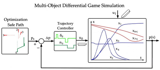
All these elements are best covered by a mathematical model of such a control process in the form of a differential game. Thus, the game control of ship 0 is along the set optimal safe trajectory ps(X, Y) running in the control system, as shown in Figure 1.
A mathematical model of such a process is necessary, both for the synthesis of a safe trajectory optimization algorithm and for the synthesis of a simulation model in the form of a differential game simulator for ships.
The algorithms of the positional game and the matrix game [23] are used to calculate the safe ship trajectory.
At the same time, in terms of interacting ships as players, three possible steering hypotheses are established: cooperative—in accordance with COLREGs, non-cooperative—in the case of an incorrect subjective assessment of the situation by the navigator, non-game—assuming that other ships are not maneuvering.
The game model is adapted to cooperate with the standard ARPA anti-collision system, which allows to track up to 20 ships; the data of the next new ships can be successively entered into the model. The positional and matrix game algorithms allow to determine the own ship safe trajectory in a dozen or so seconds in relation to 300 other ships encountered.
2.2. Ship Kinematics and Dynamics as Control Objects
The mutual movement of ships is shown in Figure 2; it is described by appropriate equations of kinematics and dynamics resulting from the hydrodynamic principles of the conservation of momentum and twist.
Applying the principle of the conservation of the momentum of the force components along the x- and y-axes, the first two general equations of the motion of ship 0 are obtained:
The third equation of the motion of ship 0 is obtained from the principle of the conservation of the turn:
In these equations, m0x is the mass of vessel 0 and accompanying water in the x-direction; m0y is the mass of vessel 0 and accompanying water in the direction of the y-axis; F0x is the geometric sum of the projections of the hydrodynamic and external forces on the x-axis; F0y is the geometrical sum of the projections of the hydrodynamic and external forces on the y-axis; J is the moment of inertia of the mass of ship 0 and accompanying water on the vertical axis of ship 0 passing through its center of gravity; and M0z is the geometric sum of the moments of hydrodynamic and external forces on the vertical axis passing through the center of gravity of ship 0.
The components of the speed of ship 0 are as follows:
To obtain the detailed equations of the ship dynamics, the components of the hydrodynamic and external forces and moments should be developed in detail. This results in the following nonlinear Pierszyc model of ship 0 dynamics [24]:
where L is the length of ship 0; Ps is the propeller thrust force; H0 is the pitch of the propeller adjuster; n0 is the rotational speed of the propeller; and q, h, r, s, and z are the coefficients of the dynamic equations of ship 0.
The non-linear dynamics of the ship as a controlled object results from the non-linear equations of the ship’s motion (4), which means that the state variables do not change in time proportionally to the control quantities. This is particularly visible when performing the anti-collision maneuver required by the COLREGs regulations, a larger change of own ship’s course noticeable by another vessel.
Equation (4) describes the nonlinear dynamics of the control of ship 0 by means of changes to the rudder angle δ0, rotational speed n0, and pitch H0 of the propulsion-adjusting screw of ship 0. Speed losses occurring during the course of change maneuvers are also obtained.
In contrast, the mathematical model of the motion of ship j uses the following kinematic equations:
Having prepared the models of the motion dynamics of ship 0 and motion kinematics of ship j, the motion of ships using state differential equations can be described.
2.3. State Equations
The properties of the control process of ships can be described by the following equation of state:
where xi,0 is the state vector of ship 0; xi,j is the state vector of ship j; ui,0 is the control vector of ship 0; and ui,j is the control vector of ship j.
Taking into account the equations of ship 0 dynamics (4) and j ship kinematics (5), the process state equations take the following form:
where x1,0 = ψ is the course of ship 0; is the angular speed of ship 0; is the drift angle of ship 0; x4,0 = V0 is the speed of ship 0; = is the x-coordinate of the distance from ship 0 to ship j; is the y-coordinate of the distance from ship 0 to ship j; = is the bearing angle of ship 0 relative to ship j; is the distance of ship 0 to ship j; is the rudder angle of ship 0; is the propeller rotational speed of ship 0; is the propeller pitch of ship 0; is the course of ship j; and is the speed of ship j.
The coefficients ai and bi contained in state Equations (1)–(8) determine the dynamics of a specific ship, depending on its deadweight, draft, length, and mass. For the purposes of this research and to conduct a simulation study of the differential game model, the values of the coefficients for a container ship with a carrying capacity of 20,000 DWT were adopted. These are presented in Table 1.
In terms of availability of data for setting the own ship dynamic equations, it is proposed, similarly to the optimization of meteorological ship routes, to calculate the equation coefficients for several typical ship size classes in advance.
3. Ship Differential Game Model in LabVIEW
The differential game state Equations (7)–(14) can be used, after their prior simplification, for the synthesis of algorithms for the safe control of an object in the game environment and to build a differential game simulation model of the multi-object-motion process used to test previously developed algorithms. Such control algorithms, developed by the author of this article using MATLAB 2023 version software, as well as a positional game model and matrix game model are described in [25]. The developed algorithms should be tested on an accurate simulation model of the game process before using them on a ship.
The most convenient tool for this purpose is LabVIEW software, which allows the simulation model to be coupled via interfaces, both with state variable measuring devices and with an external controller, to implement the game control algorithm.
LabVIEW software is a tool with much less versatility compared with the MATLAB package, but it allows for effective applications with control systems. Its main functions are related to the possibility of creating virtual interfaces of measuring devices. This is of particular importance when planning complex and long-term experiments as well as monitoring processes with a full documentation of their course. The results obtained with LabVIEW software can be used for ongoing process evaluations and analyses. This not only effectively influences the course of the process but also changes the structure. The software consists of three main modules:
- A graphical interface, the desktop;
- A structure diagram;
The LabVIEW environment provides a simple, intuitive package; programming is conducted by combining graphic elements symbolizing mathematical functions and operators as well as logical and algorithmic structures to create programs and their modifications.
A distinctive feature of the built model is the ability to conduct research in online mode. As a consequence, the end user has the ability to track the impact of changes using specific parameters of the tested system on an ongoing basis. Unlike MATLAB, the results are obtained in a short period of time. Thus, the proposed solution can observe the course of the control process with various changing operating conditions.
The possibilities of the implemented model can easily be extended; there are extensive tools that can be used to analyze the control quality and assess its sensitivity, both to the inaccuracy of the measurement of state variables and to the variability of the parameters of the control object dynamics.
3.1. State Equation Models
3.2. State Equation Computer Simulation
The time characteristics of the input and output quantities of the differential game model during the course-change maneuver of ship 0 to avoid a collision with ship j are shown in Figure 12.
As a result of the anti-collision maneuver, ships 0 and j can pass safely at a distance of .
3.3. Simulator Desktop
The view of the operating panel of the differential game simulator when the target ship passes three other encountered ships is shown in Figure 13.
The simulator allows for the movement of ship 0 along the previously determined safe trajectory in relation to the movement of the three passing ships. Ship 0 can maneuver a change of course ψ by a deflection of the rudder by angle δ0 or a change of speed V0 by changing the speed of rotation n of the propeller and its pitch H. The encountered ship maneuvers a change of course ψj or speed Vj.
4. Simulation Studies
A real navigation situation from the Skagerrak Strait—recorded using an automatic radar plotting aid (ARPA) system by SAM Raytheon Electronics installed on the research and training vessel r/v HORIZONT II during a scientific cruise to Spitsbergen—was subjected to simulation tests. Measurement data describing the situation of ship 0 passing by j = 3 other ships are included in Table 2.
The image of the examined situation in the form of ship speed vectors is shown in Figure 14.
Simulation tests were performed for the following possible conditions of mutual vessel traffic:
- Cooperative game safe control, taking into account the COLREG rules of preventing ship collisions at sea (Figure 15);
- Non-cooperative game safe control, in situations of a subjective erroneous assessment of the navigational situation or in restricted visibility conditions at sea (Figure 16);
- Optimal non-game safe control, with unchanged values of the course and speed of the ship (Figure 17).
The measure of the comparative assessment of the differential game simulation results is the value e of the deviation of the ship’s trajectory from the initial course after the completion of the game control.
From the conducted tests of the differential game simulator, it was confirmed that the largest deviation εnk of the safe trajectory existed for non-cooperative control; the smallest εk was for the cooperation of ships to avoid collisions.
The basic type of safe maneuvering is changing course. A speed change in the form of a decrease occurs when ships maintain constant speed and course values and when they do not cooperate to avoid collisions.
Compared with the method of evaluating and analyzing State-Of-The-Art human trajectory prediction (SOTA) [29], for safe and socially conscious collision prediction indicators, the differential game method allows the subjectivity of the human navigator to be taken into account in making the final maneuver decision. Trajectory prediction algorithms based on deep learning by limitation (IL) SOTAs perform much less well in some trajectory categories. SOTA methods do not exhibit collision avoidance behavior compared with game prediction methods.
5. Conclusions
The designed differential game simulator permits the following:
- The modeling of various navigational situations in terms of the risk of collision resulting from the subjectivity of the assessment of the maneuvering situation and the state of visibility at sea;
- The degree of cooperation between ships to be obtained;
- The assessment of the size of a safe trajectory deviation of a ship from an initial direction as well as the largest non-cooperative control and the smallest cooperation of ships to avoid collisions;
- The feasibility of a previously determined safe trajectory of a ship to be checked, based on the algorithm of the positional or matrix games;
- The synthesis of new control algorithms using artificial intelligence methods;
- The practical training of navigators to prevent ship collisions at sea.
Further research is needed to expand the simulator for a larger number of ships and to test the sensitivity of the game control quality to inaccuracies in the measured state variables and to changes in the parameters of the ship’s dynamics.
Funding
This research was funded by the research project “Control algorithms synthesis of autonomous objects” No. WE/2023/PZ/02, Electrical Engineering Faculty, Gdynia Maritime University, Poland.
Data Availability Statement
This study did not report any data.
Conflicts of Interest
The author declares no conflict of interest.
References
- Marden, J.R.; Shamma, J.S. Game theory and control. Annu. Rev. 2018, 1, 105–134. [Google Scholar] [CrossRef]
- Sani, M.; Robu, B.; Hably, A. Limited information model predictive control for pursuit-evasion games. In Proceedings of the 60th IEEE Conference on Decision and Control (CDC), Austin, TX, USA, 13–17 December 2021; pp. 265–270. [Google Scholar] [CrossRef]
- Gong, Z.; He, B.; Liu, G.; Zhang, X. Solution for Pursuit-Evasion Game of Agents by Adaptive Dynamic Programming. Electronics 2023, 12, 2595. [Google Scholar] [CrossRef]
- Guo, X.; Guo, A.; Zhao, S. Null-Space-Based Multi-Player Pursuit-Evasion Games Using Minimum and Maximum Approximation Functions. Electronics 2022, 11, 3729. [Google Scholar] [CrossRef]
- Lisowski, J. A Synthesis of Algorithms Determining a Safe Trajectory in a Group of Autonomous Vehicles Using a Sequential Game and Neural Network. Electronics 2023, 12, 1236. [Google Scholar] [CrossRef]
- Isaacs, R. Differential Games: A Mathematical Theory with Applications to Warfare and Pursuit, Control and Optimization; Dover Publications: New York, NY, USA, 1999; ISBN 0-486-40682-2. [Google Scholar]
- Mikulski, L.; Kropiowska, D. Usage of a zero-sum differential game in the optimal control of an object described by a nonlinear model. Tech. Trans. Civ. Eng. 2018, 9, 109122. [Google Scholar]
- Yanan, L.; Gerolamo, C.; Franck, G.; Domenico, C.; Etienne, B. Differential game theory for versatile physical interaction. Nat. Mach. Intell. 2019, 1, 36–43. [Google Scholar] [CrossRef]
- Gajarsky, J.; Gorsky, M.; Kreutzer, S. Differential Games, Locality, and Model Checking for FO Logic of Graphs. In Proceedings of the 30th EACSL Annual Conference on Computer Science Logic, Gottingen, Germany, 14–19 February 2022. [Google Scholar] [CrossRef]
- Sani, M.; Hably, A.; Robu, B.; Dumon, J.; Meslem, N. Experiments on the control of differential game of target defense. In Proceedings of the ECC—21st European Control Conference, Bucharest, Romania, 13–16 June 2023; Available online: https://hal.science/hal-04153630 (accessed on 5 August 2023).
- Gammoudi, N.; Zidani, H. A differential game control problem with state constraints. Math. Control Relat. Fields 2023, 13, 554–582. [Google Scholar] [CrossRef]
- Mylvaganam, T.; Sassano, M.; Astolfi, A. A differential game approach to multi-agent collision avoidance. IEEE Trans. Autom. Control 2017, 62, 4229–4235. [Google Scholar] [CrossRef]
- Turetsky, V.; Hayoun, S.Y.; Shima, T.; Tarasyev, A. On the value of differential game with asymmetric control constraints. IFAC-PapersOnLine 2018, 51, 799–804. [Google Scholar] [CrossRef]
- Ougolnitsky, G.; Usov, A. Spatially Distributed Differential Game Theoretic Model of Fisheries. Mathematics 2019, 7, 732. [Google Scholar] [CrossRef]
- Gong, Z.; He, B.; Hu, C.; Zhang, X.; Kang, W. Online Adaptive Dynamic Programming-Based Solution of Networked Multiple-Pursuer and Single-Evader Game. Electronics 2022, 11, 3583. [Google Scholar] [CrossRef]
- Li, Y.; Hu, X. A differential game approach to intrinsic formation control. Automatica 2022, 136, 110077. [Google Scholar] [CrossRef]
- Engwerda, J. Min-Max Robust Control in LQ-Differential Games. Dyn. Games Appl. 2022, 12, 1221–1279. [Google Scholar] [CrossRef]
- Cappello, D.; Mylvaganam, T. Distributed Differential Games for Control of Multi-Agent Systems. IEEE Trans. Control Netw. Syst. 2022, 9, 635–646. [Google Scholar] [CrossRef]
- Wang, X.; Ma, Z.; Mao, L.; Sun, K.; Huang, X.; Fan, C.; Li, J. Accelerating Fuzzy Actor–Critic Learning via Suboptimal Knowledge for a Multi-Agent Tracking Problem. Electronics 2023, 12, 1852. [Google Scholar] [CrossRef]
- Kaklis, D.; Varlamis, I.; Giannakopoulos, G.; Varelas, T.J.; Spyropoulos, C.D. Enabling digital twins in the maritime sector through the lens of AI and industry 4.0. Int. J. Inf. Manag. Data Insights 2023, 3, 00178. [Google Scholar] [CrossRef]
- Gkerekos, C.; Lazakis, I. A novel, data-driven heuristic framework for vessel weather routing. Ocean. Eng. 2020, 197, 106887. [Google Scholar] [CrossRef]
- Lisowski, J. The dynamic game theory methods applied to ship control with minimum risk of collision. Risk Anal. V Simul. Hazard Mitig. 2006, 91, 293–302. [Google Scholar] [CrossRef]
- Lisowski, J. Game Control Methods Comparison when Avoiding Collisions with Multiple Objects Using Radar Remote Sensing. Remote Sens. 2020, 12, 1573. [Google Scholar] [CrossRef]
- Gierusz, W. Simulation Model of the Shiphandling Training Boat “Blue Lady”. IFAC Proc. Vol. 2001, 34, 255–260. [Google Scholar] [CrossRef]
- Lisowski, J. Synthesis of a Path-Planning Algorithm for Autonomous Robots Moving in a Game Environment during Collision Avoidance. Electronics 2021, 10, 675. [Google Scholar] [CrossRef]
- NI. State-Space Model Definitions (Advanced Signal Processing Toolkit or Control Design and Simulation Module). Available online: https://www.ni.com/docs/en-US/bundle/labview-advanced-signal-processing-toolkit-api-ref/page/lvsysidconcepts/modeldefinitionsss.html (accessed on 24 July 2023).
- NI. Estimating and Validating a State-Space Model (Advanced Signal Processing Toolkit or Control Design and Simulation Module). Available online: https://www.ni.com/docs/en-US/bundle/labview-control-design-and-simulation-module/page/lvsysidconcepts/case_study_ssest.html (accessed on 25 July 2023).
- NI. Defining a Cost Function (Control Design and Simulation Module). Available online: https://www.ni.com/docs/en-US/bundle/labview-control-design-and-simulation-module/page/lvsimconcepts/sim_c_costfunc.html (accessed on 25 July 2023).
- Wang, E.; Hoshino, H.; Ramanan, D.; Kitani, K. Joint Metrics Matter: A Better Standard for Trajectory Forecasting; Cornell University: New York, NY, USA, 2023. [Google Scholar] [CrossRef]
Figure 1.
Control system of the ship game control: ps is the assigned trajectory of ship 0 in the coordinate system (X,Y); p is the actual trajectory of ship 0; Δp is the deviation of position of ship 0 from the assigned voyage route; u0 is the control of ship 0 by a deflection of the rudder δ0, which changes the rotational speed of the propeller n0 and pitch H0 of the propeller for the propulsion of the ship; uj controls ship j by changing its course ψj and speed Vj; and xj is a quantity describing the position of the ships relative to each other in the form of distance Dj and bearing Nj.

Figure 2.
Quantities characterizing the course of the ship control process: δ0 is the rudder deflection of ship 0; ψ0 is the course of ship 0; V0 is the speed of ship 0; β0 is the drift angle of ship 0; (V0x, V0y) are components of the velocity of ship 0; Dj is the distance to ship j; Nj is the bearing of the relative direction of ship j; Vj is the speed of ship j; ψj is the course of ship j; Djmin is the shortest passing distance between ships; and Tjmin is the time until the largest convergence of the ships.

Figure 3.
Scheme of the model of state equations of differential game of ships using LabVIEW software.
Figure 3.
Scheme of the model of state equations of differential game of ships using LabVIEW software.

Figure 4.
State Equation (7) modeled using LabVIEW to obtain state variable x1,0.

Figure 5.
State Equation (8) modeled using LabVIEW to obtain state variable x2,0.

Figure 6.
State Equation (9) modeled using LabVIEW to obtain state variable x3,0.

Figure 7.
State Equation (10) modeled using LabVIEW to obtain state variable x4,0.

Figure 8.
State Equation (11) modeled using LabVIEW to obtain state variable x5,j.

Figure 9.
State Equation (12) modeled using LabVIEW to obtain state variable x6,j.

Figure 10.
State Equation (13) modeled using LabVIEW to obtain state variable x7,j.

Figure 11.
State Equation (14) modeled using LabVIEW to obtain state variable x8,j.

Figure 12.
Changes over time of state vector variables x and control vector u during the anti-collision maneuver.
Figure 12.
Changes over time of state vector variables x and control vector u during the anti-collision maneuver.

Figure 13.
Desktop of simulator with settings of control quantities.

Figure 14.
Navigation scenario of the movement of ship 0 and three j ships encountered.

Figure 15.
Simulation of a cooperative differential game: (a) ship 0 control in the form of rudder deflection δ0 and (b) propeller speed n0; (c) ships j steering in the form of course ψj and (d) speed Vj; and (e) trajectories of ship 0 and ships j. εc is the safe trajectory deviation from an assigned direction.

Figure 16.
Simulation of a non-cooperative differential game: (a) ship 0 control in the form of rudder deflection δ0 and (b) propeller speed n0; (c) ships j steering in the form of course ψj and (d) speed Vj; and (e) trajectories of ship 0 and ships j. εnc is the safe trajectory deviation from an assigned direction.

Figure 17.
Simulation of a non-game optimal control: (a) ship 0 control in the form of rudder deflection δ0 and (b) propeller speed n0; (c) ships j steering in the form of course ψj and (d) speed Vj; and (e) trajectories of ship 0 and ships j. εng assigned direction. ![Electronics 12 03848 i001]() : speed V0 of ship 0 reduced by 25%.
: speed V0 of ship 0 reduced by 25%.
 : speed V0 of ship 0 reduced by 25%.
Figure 17.
Simulation of a non-game optimal control: (a) ship 0 control in the form of rudder deflection δ0 and (b) propeller speed n0; (c) ships j steering in the form of course ψj and (d) speed Vj; and (e) trajectories of ship 0 and ships j. εng assigned direction. ![Electronics 12 03848 i001]() : speed V0 of ship 0 reduced by 25%.
: speed V0 of ship 0 reduced by 25%.
: speed V0 of ship 0 reduced by 25%.

Table 1.
Coefficient values of state equations for a 20,000 DWT container ship.
| Coefficient | Value | Coefficient | Value |
|---|---|---|---|
| a1 (m−1) | 41.4 | a10 (s−1) | 0.93 |
| a2 (m−2) | 0.19 | b1 (m−2) | 113 |
| a3 (m−1) | 62.0 | b2 (m−1) | 1.55 |
| a4 (m−1) | 44.2 | b3 (s−1) | 1.45 |
| a5 | 6.93 | b4 (s−1) | 1.36 |
| a6 | 31.8 | b4+j (s−1 m−1) | 10.0 |
| a7 (m−1) | 89.0 | b5+j (s m−2) | 0.80 |
| a8 | 44.1 | b6+j (m−1) | 95.2 |
| a9 | 44.3 |
Table 2.
Values of quantities characterizing the navigational situation.
| Ship j | Speed Vj (kn) | Course ψj (deg) | Coordinate Xj (nm) | Coordinate Yj (nm) |
|---|---|---|---|---|
| 0 | 20.0 | 0 | 0 | 0 |
| 1 | 14.5 | 090 | −5.2 | 7.3 |
| 2 | 16.2 | 180 | 1.1 | 8.4 |
| 3 | 16.0 | 200 | 1.6 | 7.6 |
Disclaimer/Publisher’s Note: The statements, opinions and data contained in all publications are solely those of the individual author(s) and contributor(s) and not of MDPI and/or the editor(s). MDPI and/or the editor(s) disclaim responsibility for any injury to people or property resulting from any ideas, methods, instructions or products referred to in the content. |
© 2023 by the author. Licensee MDPI, Basel, Switzerland. This article is an open access article distributed under the terms and conditions of the Creative Commons Attribution (CC BY) license (https://creativecommons.org/licenses/by/4.0/).
Share and Cite
MDPI and ACS Style
Lisowski, J. Nonlinear Multi-Object Differential Game Simulation Model in LabVIEW. Electronics 2023, 12, 3848. https://doi.org/10.3390/electronics12183848
AMA Style
Lisowski J. Nonlinear Multi-Object Differential Game Simulation Model in LabVIEW. Electronics. 2023; 12(18):3848. https://doi.org/10.3390/electronics12183848
Chicago/Turabian StyleLisowski, Józef. 2023. "Nonlinear Multi-Object Differential Game Simulation Model in LabVIEW" Electronics 12, no. 18: 3848. https://doi.org/10.3390/electronics12183848
Note that from the first issue of 2016, this journal uses article numbers instead of page numbers. See further details here.