Adaptive Fast-Terminal Neuro-Sliding Mode Control for Robot Manipulators with Unknown Dynamics and Disturbances

Abstract

This paper presents a novel adaptive fast-terminal neuro-sliding mode control (AFTN-SMC) for a two-link robot manipulator with unknown dynamics and external disturbances. The proposed controller is chattering-free and adaptive to the time-varying system uncertainties. Furthermore, the radial base function neural network (RBFNN) is employed to approximate the unknown state dynamics. The simulations have been completed in MATLAB, which illustrates the successful implementation of the proposed controller. The results showcased the effectiveness of the AFTN-SMC in achieving accurate tracking and stability, even in the presence of uncertainties and parameter variations. The incorporation of the RBFNN in the controller proved to be a valuable tool for approximating the unknown dynamics, enabling accurate estimation and control of the manipulator’s behavior. The research presented in this paper contributes to the advancement in control techniques for robot manipulators in diverse industrial and automation applications.

1. Introduction

Robot manipulators are extensively being used for a diverse range of applications, like the automation industry, manufacturing, space, military, and robotic surgery [1,2,3]. The versatility and adaptability of robot manipulators have allowed them to revolutionize multiple industries and provide invaluable support in diverse scenarios. The robot manipulator is a device that is applied to operate materials without physical contact with the operator. The main purpose of these manipulators was originally to handle radioactive or hazardous materials, but now it is extended to industrial applications as well [1]. The manipulator assists operators in lifting materials that are either heavy, hot, or difficult to manually handle. One notable area where robot manipulators have made a significant impact is in the field of logistics and warehousing. With the rise of e-commerce and the increasing demand for efficient order fulfillment, companies have turned to automation solutions to streamline their operations. Robot manipulators have emerged as essential tools in these environments, enabling the swift and accurate handling of goods. These manipulators are capable of picking, placing, and sorting items with precision, enhancing productivity and minimizing errors in the process.

Moreover, the use of robot manipulators has extended to hazardous environments, where the safety and well-being of human operators are at risk. For instance, in nuclear power plants, these manipulators are employed to handle radioactive materials, ensuring the protection of workers from potential radiation exposure. Similarly, in chemical plants or other hazardous industrial settings, robot manipulators allow for the manipulation of dangerous substances without endangering human lives. By providing remote operation capabilities, these devices enable operators to perform tasks from a safe distance, mitigating potential risks and ensuring a safer working environment.

Based on the combination of joints and configurations, there exist various forms of manipulators, each designed to suit specific applications and operational requirements. Robot manipulators can be broadly categorized into two main types: single-link and multi-link robot manipulators. Single-link manipulators consist of a single arm or limb with one degree of freedom, allowing for simple linear motion along a single axis. Due to their relatively simpler structure and limited degrees of freedom, single-link manipulators have been extensively studied and well-documented in scientific research. On the other hand, multi-link manipulators are characterized by having multiple arms or limbs, each with its own set of joints and degrees of freedom. These manipulators offer increased flexibility and versatility, enabling complex motions and operations. However, the complexity associated with multi-link systems presents challenges in terms of control and modeling.

Scientific research on robot manipulators has primarily focused on single-link manipulators due to their relative simplicity. This narrower focus has allowed for a deeper understanding of their dynamics, control algorithms, and trajectory planning. In contrast, the study of multi-link manipulators has been more limited due to their increased complexity, nonlinear dynamics, and higher degrees of freedom. Efficient control systems for multi-link manipulators are crucial to effectively manage their flexible nature and enable precise and accurate manipulation. Developing an adaptive mathematical framework for modeling multi-link manipulators becomes essential in order to account for the nonlinear dynamics and dynamic interactions between the links [4,5].

The complexity of multi-link manipulators further intensifies when they are tasked with carrying a payload. The additional weight and inertia of the payload influence the manipulator’s dynamics and require careful consideration in terms of control and stability. The control system must account for the effects of the payload, ensuring that the manipulator can perform tasks accurately and reliably. In practical applications, multi-link manipulators are often required to perform tasks following a specific trajectory or a series of assigned positions. These tasks can involve various types of movements, such as pick-and-place operations, assembly tasks, or complex maneuvers. Allocating a specific trajectory for the manipulator to follow allows for precise control and coordination of its movements, ensuring efficient and effective task execution.

Multi-link manipulators outperform single-link in terms of performance. The single-link robot manipulator has restricted execution compared to multi-link due to its utilization of appropriate controllers. The controller for the multi-link faces nonlinear dynamic and external disturbances while performing tasks [6]. To address the nonlinear dynamic issue, there is a need for more scientific work on the controller design for multi-link robot manipulators [7]. The two-link (multi-link) robot manipulators are appropriate in industries such as aviation, manufacturing, military, and automotive. Therefore, it is important to conduct further research on two-link manipulators in terms of dynamical complexities, modeling, and controller design [7,8,9].

There are several control techniques presented to control the robot manipulators. Proportional–integral–derivative controller (PID) control [10,11,12], fuzzy logic control [11,12,13,14,15,16], neural network control [17,18], sliding mode control (SMC) [19,20,21], and adaptive control [13,14,15] are some of the scientific research techniques being used for the controller. PID control takes minimal effort to implement; however, it lacks self-adaptation capability, resulting in high energy consumption. The research by the authors in [19,22] based on adaptive control methods can change control algorithms based on the external environment. The downside is that a precise mathematical model is needed to construct the controller. Similarly, the research findings on feedback linearizing [23,24] are efficient in following control of the nonlinear systems. Due to the model employing matrix inversion, it takes more time for calculation, and, additionally, it needs model-based information for the controller.

The research on robust control such as SMC is presented by the author in [21], which overcomes uncertainties and external disturbances. The SMC method is considered by researchers because the desired trajectory is tracked by achieving a predefined sliding surface and the system then attains equilibrium based on it. The switching signal with high gain is used to achieve a predefined surface; however, this signal produces chattering problems and potentially can damage the actuators. The damage can render the system unstable and reduce the controller’s performance.

In order to overcome the chattering issue, the standard method is the employment of a boundary layer around the surface. This boundary layer in return has a larger response time and therefore needs to be balanced. The research by the author [25] on terminal SMC achieves finite-time convergence compared to conventional SMC due to nonlinear sliding surfaces.

Moreover, it is challenging or even impossible to obtain accurate information about the states of a robot manipulator. Consequently, when designing a robot manipulator, it becomes necessary to estimate these states. In order to address this challenge, this research paper introduces a novel approach using a neural network for state estimation. This neural-network-based method is employed to design a controller that can effectively operate the robot manipulator. By leveraging the capabilities of the neural network, the proposed controller can compensate for the lack of precise state information and still achieve reliable performance.

The main contribution of this paper is to design the adaptive fast-terminal neuro-SMC (AFTN-SMC) for unknown dynamics and external disturbance for a two-link robot manipulator. The proposed controller is chattering-free and adaptive to the time-varying system uncertainties. Furthermore, the radial base function neural network (RBFNN) is employed to approximate the unknown state dynamics. The simulation has been completed in MATLAB, which illustrates the implementation of the proposed controller.

The rest of the paper is assembled as follows: Section 2 includes the dynamic model of a two-link robot manipulator, including the preliminaries and problem formation. Section 3 proposes the adaptive fast-terminal neuro-sliding mode control along with the main results. Section 4 comprises the simulation of the proposed controller using the MATLAB environment. Furthermore, Section 5 includes the conclusion and future work.

2. Preliminaries and Problem Formation

2.1. Preliminaries

This section includes basic lemmas, definitions, and assumptions that will be used in this paper. The dynamical equation of a nonlinear system is provided below:

$$\dot{x}\left(t\right)=F(t,x),x\left(0\right)=x_0,$$

(1)

where $x\in R^n$ and $F\left(x\right):R^n\to R^n$ is a nonlinear function and the following lemmas and definitions are established for Equation (1) [26,27]. If there is a continuous and differentiable positive definite function $V\left(x\right):R^n\to R$, such that

$$\begin{array}{c}\hfill \dot{V}\left(x\right)\le -{\omega }_{1}V\left(x\right)-{\omega }_2{V}^z\left(x\right),\end{array}$$

(2)

where ${\omega }_1>0$, ${\omega }_2>0$, and $0<z<1$, then the settling time is provided by

$$\begin{array}{c}\hfill T\le \frac{1}{{\omega }_1(1-z)}ln\frac{{\omega }_1{V}^{1-z}\left(x_0\right)+{\omega }_2}{{\omega }_2},\end{array}$$

(3)

Reference [28] for $s_i\in R,i=1,2,...,n,0<\beta \le 1$, following relationship exists:

$$\begin{array}{c}\hfill {s\left|s\right|}^{\beta }sgn\left(s\right)\le \sum _{i=1}^n{\left(s_i^2\right)}^{\frac{1+\beta }{2}},\end{array}$$

(4)

The desired trajectory $q_d$ and its first and second derivatives are bounded, such that $|q_d|\le {\gamma }_0\left(t\right)$ and $|q_d^{\left(i\right)}|\le {\gamma }_i\left(t\right)$, $i\in \{1,2\};\forall t>0$.

The unknown disturbance $d_i$ is bounded, such that $|d_i|\le D_i,i\in \{1,2\};\forall t>0$ and $D_i$ is known positive constant.

The system uncertainties and external disturbances are provided by

$$\begin{array}{c}\hfill D(q,\dot{q},\ddot{q})<{\beta }_1+{\beta }_2\parallel q\parallel +{\beta }_3{\parallel \dot{q}\parallel }^2,\end{array}$$

(5)

where ${\beta }_1,{\beta }_2$, and ${\beta }_3$ are unknown positive constants.

Assume that a constant $k_{adp}$ exists such that $|k_{adp}|\ge \frac{1}{\left|s\right|}\left({\beta }_1+{\beta }_2\parallel q\parallel +{\beta }_3{\parallel \dot{q}\parallel }^2\right)$.

2.2. Problem Formation

The general form of the dynamic equation for a multi-link robot manipulator is provided below:

$$M\left(q\right)\ddot{q}+F(q,\dot{q})\dot{q}+G\left(q\right)=u+d,$$

(6)

where $M\left(q\right),F(q,\dot{q})$, and $G\left(q\right)$ are the inertia matrix, centripetal Coriolis matrix, and gravitational vector, respectively. These terms represent the nonlinear dynamics of the system. Further, u and d are designed to control signals and unknown external disturbances, respectively. $q,\dot{q}$, and $\ddot{q}$ are the vectors of order $R^n$, representing the joint positions, velocities, and accelerations, respectively. In the case of a two-link robot manipulator, n will be 2, where n represents the number of links in multi-link robot manipulators.

Figure 1 illustrates a two-link robot manipulator, showcasing its physical structure and motion characteristics. The dynamics of this manipulator are described by the nonlinear Equation (6), which governs its behavior and movement. The two links of the manipulator are represented by $m_a$ and $m_b$, indicating their respective masses, while $r_a$ and $r_b$ denote the lengths of the first and second joints, respectively. The positions of the first angle, $q_a$, are measured with respect to the inertial frame of the first link, while the second angle, $q_b$, is measured with respect to the orientation frame of the second link. These angles define the configuration of the manipulator and determine its position in space.

To control the manipulator’s movements, designed control signals $u_a$ and $u_b$ are applied to the actuators. These control signals determine the torque or force applied to the joints, enabling the robot to execute desired motions and perform specific tasks. By manipulating the control signals, operators or control systems can regulate the manipulator’s position, velocity, and acceleration.

When the control signals are transmitted to the actuators, the robot manipulator responds by initiating the desired motion. The actuators generate the necessary forces or torques to drive the joints and links, resulting in the manipulator moving according to the specified control signals. The precise coordination and synchronization of these control signals enable the manipulator to perform complex and intricate tasks with accuracy and efficiency.

Understanding the dynamics of the robot manipulator and its response to control signals is crucial for designing effective control strategies. By analyzing the nonlinear Equation (6) and considering the physical parameters of the manipulator, researchers and engineers can develop control algorithms that optimize the manipulator’s performance, enhance its stability, and ensure the achievement of desired task objectives.

Uncertainties always exist in real systems; therefore, in this paper, we consider the uncertain system dynamics, such as $M\left(q\right)=M_0\left(q\right)+\delta m$, $F(q,\dot{q})=F_0(q,\dot{q})+\delta f$, and $G\left(q\right)=G_0\left(q\right)+\delta g$, where $\delta m,\delta f$, and $\delta g$ are the uncertain parts of the nonlinear dynamics and $M_0\left(q\right),F_0(q,\dot{q})$, and $G_0\left(q\right)$ are the nominal parts. Equation (6) for the uncertain dynamical system can be written as follows:

$$M_0\left(q\right)\ddot{q}+F_0(q,\dot{q})\dot{q}+G_0\left(q\right)=u+D(q,\dot{q},\ddot{q}),$$

(7)

where $D(q,\dot{q},\ddot{q})=d-\delta m\ddot{q}-\delta f\dot{q}-\delta g$ is the perturbation. Perturbation in a dynamic system refers to a small deviation or disturbance from the system’s equilibrium or desired state. These perturbations can arise from different sources, such as initial conditions, external forces, parameter variations, or actuator imperfections. For instance, a perturbation can occur by introducing a slight deviation in the initial joint angles or velocities of the manipulator. Additionally, external forces or disturbances, such as unexpected contact forces or environmental factors, may act on the system during operation. Moreover, uncertainties in the physical parameters of the manipulator or imperfections in the actuators can further contribute to perturbations. To ensure robust and accurate control of the manipulator’s motion, a robust fast-terminal neuro-sliding mode control with unknown states is employed to mitigate the effects of these perturbations. By accounting for and compensating for perturbations, the manipulator’s stability, precision, and overall performance are maintained, even in the presence of uncertainties. It can be introduced intentionally or occur naturally due to external factors or uncertainties in the system. Equation (7) can be rewritten in the form of second-order state space as follows:

$$\begin{array}{cc}\hfill {\dot{q}}_a& =q_b\hfill \\ \hfill {\dot{q}}_b& =-X(q,\dot{q})+Y\left(q\right)u+D_0(q,\dot{q},\ddot{q}),\hfill \end{array}$$

(8)

where $q={[q_a,q_b]}^T$ includes the second-order vectors for joint positions. $X(q,\dot{q})=M_0^{-1}\left(q\right)(F_0(q,\dot{q})\dot{q}+G_0\left(q\right))$ includes unknown nonlinear dynamics for the two-link robot manipulator, $Y\left(q\right)=M_0^{-1}\left(q\right)$ is control gain matrix, and $D_0(q,\dot{q},\ddot{q})=M_0^{-1}\left(q\right)D(q,\dot{q},\ddot{q})$ is composed of system uncertainties and external disturbances.

Equation (8) represents the unknown second-order dynamics of the two-link robot manipulator with parameter uncertainties and external disturbances.

3. Main Results

3.1. Sliding Surface

In sliding mode control, a sliding surface is a key concept used to design the control law and achieve robust and accurate control of a dynamic system. The sliding surface acts as a virtual plane or hypersurface in the system’s state space, guiding the system’s trajectory toward a desired behavior. Figure 2 illustrates the sliding surface considered to design the proposed controller in this paper.

The sliding surface is defined based on the system’s state variables and desired reference vector $q_d$. It is typically chosen to have a specific mathematical form that ensures the system’s dynamics converge to the desired behavior. The selection of the sliding surface depends on the specific system and control objectives.

The primary characteristic of the sliding surface is that it divides the state space into two distinct regions: the chattering phenomena and the finite-time reaching phase, as shown in Figure 2. In the sliding mode, the system’s trajectory is constrained to the sliding surface, and the control action is designed to keep the system on this surface. The reaching mode, on the other hand, represents the transient phase during which the system transitions from its initial state to the sliding mode.

The control law associated with sliding mode control is designed to drive the system’s trajectory toward the sliding surface and ensure that it stays on this surface. This control law often includes a discontinuous or switching term that acts to “slide” the system along the sliding surface. The control action changes abruptly when the system’s state crosses the sliding surface, ensuring robustness to uncertainties and disturbances.

Let us consider the desired position vector $q_d\in R^2$ to form the error signal, such as $e=q-q_d$. Then, the sliding surface is chosen as follows for the two-link robot manipulator:

$$s=\dot{e}+\theta ,$$

(9)

where $\theta$ is an integral term and consists of a continuous function of error. The dynamical representation for $\theta$ is provided below:

$$\dot{\theta }=k_1|\dot{e}{|}^{{\alpha }_1}sign\left(\dot{e}\right)+k_2{\left|e\right|}^{{\alpha }_2}sign\left(e\right),$$

(10)

where $k_1$ and $k_2$ are positive sliding gains. ${\alpha }_1$ and ${\alpha }_2$ are positive constants. It is noted that the ${\alpha }_1$ and ${\alpha }_2$ are kept less than one to nullify the chattering effect, i.e., $0<{\alpha }_1<1$ and $0<{\alpha }_2<1$.

3.2. Radial Basis Function Neural Networks

Neural networks are extensively used to approximate unknown functions due to their excellent properties of approximation and learning capabilities. RBFNN is a type of artificial neural network that has shown effectiveness in various applications, including state estimation. RBFNNs are characterized by their use of radial basis functions as activation functions in the hidden layer. In state estimation, RBFNNs can be utilized to estimate the states of a dynamic system based on available sensor measurements. The RBFNN is trained using a set of input–output data pairs, where the inputs represent the sensor measurements and the outputs represent the corresponding states of the system.

The RBFNN consists of three layers (Figure 3): an input layer, a hidden layer with radial basis functions as activation functions, and an output layer. The input layer receives the sensor measurements as inputs, which are then passed through the hidden layer. The hidden layer computes the activations of the radial basis functions, which are centered at specific points in the input space. These radial basis functions transform the input space into a higher-dimensional feature space.

The output layer of the RBFNN performs a linear combination of the activations from the hidden layer to produce the estimated states as the final output. The output layer approximates the unknown continuous nonlinear function $X(q,\dot{q})$ such that:

$$X(q,\dot{q})=W^T\theta (q,\dot{q})+\mu ,$$

(11)

where $\mu$ is an approximation error, $W^T\in R^n$ is the output weigh vector of first layer, $\theta (q,\dot{q})$ is a vector that consists of activation functions such that $\theta (q,\dot{q})={[{\theta }_1(q,\dot{q}),{\theta }_2(q,\dot{q}),...,{\theta }_n(q,\dot{q})]}^T$, provided by

$${\theta }_k(q,\dot{q})=exp\left(\frac{-|{\theta }_i-c_k{|}^2}{2b_k^2}\right),$$

(12)

where $k=1,2,...,n$, ${\theta }_i={\left[q_i{\dot{q}}_i\right]}^T$, $c_k\in R^2$ and $b_k\in R$ are the center and width of the activation function. The activation function given in Equation (12) is a Gauss radial basis function.

The main goal of RBFNN is to minimize the approximation error $\mu$ such that:

$$X(q,\dot{q})\approx W^T\theta (q,\dot{q}),$$

(13)

The approximated output of the RBFNN serves as a crucial component in the design of the controller. It provides valuable information about the system’s behavior and aids in the generation of the control signals required to achieve the desired system response. The control law, incorporating the RBFNN output, defines how the system should react and adjusts its state based on the estimated dynamics.

By utilizing the RBFNN approximation, the proposed controller benefits from the ability of the neural network to capture nonlinear relationships and generalize from training data. This enables the controller to adapt to the specific system dynamics and uncertainties, resulting in improved accuracy and performance.

3.3. Proposed Controller

The design of the proposed control law involves several steps, beginning with the calculation of the first derivative of the sliding surface. This derivative is set equal to zero to obtain the equivalent controller. Subsequently, an adaptive controller is introduced to modify the equivalent controller and complete the design of the proposed control law.

Taking the first derivative of the sliding surface allows for a deeper understanding of the system dynamics and aids in the development of an effective control strategy. By equating the derivative to zero, the equivalent controller is derived, which represents the ideal control input necessary to maintain the system on the sliding surface. The first derivative of the sliding surface along the uncertain dynamical system (8) is provided below:

$$\dot{s}=-X(q,\dot{q})+Y\left(q\right)u+D_0(q,\dot{q},\ddot{q})-{\ddot{q}}_d+\dot{\theta },$$

(14)

The traditional sliding mode control signal for a known dynamical system is generated by substituting Equation (14) equal to zero as follows:

$$u=(Y{\left(q\right)}^{-1})(X(q,\dot{q})+{\ddot{q}}_d-\dot{\theta }-D_0(q,\dot{q},\ddot{q})),$$

(15)

In this paper, we have considered the improved control algorithm that is chattering-free and fast-time convergent. An adaptive control law is also employed to neutralize the dynamic uncertainties and external disturbances. Furthermore, the dynamics of the two-link robot manipulator are unknown and estimated by using RBFNN.

The combination of the equivalent controller and the adaptive controller forms the proposed control law. This integrated approach ensures that the system remains on the sliding surface while also accounting for dynamic changes in the system and adapting to the varying uncertainties. By employing this control law, the system can achieve desired tracking and stability even in the presence of uncertainties and disturbances. The overall proposed control algorithm is provided below:

$$u=u_{eq}+u_{adp},$$

(16)

where $u_{eq}$ is the equivalent control signal, provided as

$$u_{eq}=(Y{\left(q\right)}^{-1})(W^T\theta (q,\dot{q})+{\ddot{q}}_d-\dot{\theta })-k_3{\left|s\right|}^{{\alpha }_3}sign\left(s\right),$$

(17)

where $k_3$ and ${\alpha }_3$ are positive constants and the continuous term $k_3{\left|s\right|}^{{\alpha }_3}sign\left(s\right)$ enhances the performance of the proposed control algorithm. $W^T\theta (q,\dot{q})$ is the estimation of unknown nonlinear dynamics $X(q,\dot{q})$.

The adaptive controller introduces adaptive mechanisms that estimate and account for time-varying uncertainties and disturbances. By adapting the control law based on the estimated uncertainties, the adaptive controller enhances the robustness and performance of the overall control system. $u_{adp}$ is the adaptive part of the proposed control method that helps to neutralize the dynamical uncertainties and external disturbances. The adaptive control signal is provided by the following equation:

$$u_{adp}=\left\{\begin{array}{c}-\frac{s}{\left|s\right|}\left(\widehat{{\beta }_1}+\widehat{{\beta }_2}\parallel q\parallel +\widehat{{\beta }_3}{\parallel \dot{q}\parallel }^2\right)\left|s\right|\ge {\delta }_0\hfill \\ -\frac{s}{{\delta }_0^2}\left(\widehat{{\beta }_1}+\widehat{{\beta }_2}\parallel q\parallel +\widehat{{\beta }_3}{\parallel \dot{q}\parallel }^2\right)\left|s\right|<{\delta }_0\hfill \end{array}\right.,$$

(18)

where $\widehat{{\beta }_1},\widehat{{\beta }_2}$, and $\widehat{{\beta }_3}$ are adaptive terms and provided by

$$\left\{\begin{array}{c}\dot{\widehat{{\beta }_1}}=c_{11}\widehat{{\beta }_1}+c_{12}\left|s\right|\hfill \\ \dot{\widehat{{\beta }_2}}=c_{21}\widehat{{\beta }_2}+c_{22}\left|s\right|\parallel q\parallel \hfill \\ \dot{\widehat{{\beta }_3}}=c_{31}\widehat{{\beta }_3}+c_{32}\left|s\right|\parallel \dot{q}\parallel \hfill \end{array}\right.,$$

(19)

where $\parallel .\parallel$ is the norm and $c_{11},c_{12},c_{13},c_{21},c_{22},c_{23},c_{31},c_{32}$, and $c_{33}$ are designed constants.

3.4. Stability Analysis

Equation (14) can be written as follows, together with the proposed control algorithm (16) and RBFNN-based approximation of unknown continuous nonlinear function $X(q,\dot{q})$ (13):

$$\dot{s}=Y\left(q\right)(-k_3{\left|s\right|}^{{\alpha }_3}sign\left(s\right)+u_{adp})+D_0(q,\dot{q},\ddot{q}),$$

(20)

where $Y\left(q\right)$ is a positive definite function that leads Equation (20) as follows:

$$\dot{s}\le -k_3{\left|s\right|}^{{\alpha }_3}sign\left(s\right)+u_{adp}+D(q,\dot{q},\ddot{q}).$$

(21)

To validate the stability criteria for the closed-loop dynamical system, consider the following positive definite Lyapunov function.

$$V=\frac{1}{2}{s}^{T}s+\sum _{i=1}^3\frac{{\widetilde{{\beta }_i}}^2}{2},$$

(22)

where estimation error for ${\beta }_i$ is provided by

$$\widetilde{{\beta }_i}={\beta }_i-{\widehat{\beta }}_i.$$

(23)

The derivative of the positive definite Lyapunov function given in Equation (22) is written as

$$\dot{V}\le s^T(-k_3{\left|s\right|}^{{\alpha }_3}sign\left(s\right)+u_{adp}+D(q,\dot{q},\ddot{q}))-\sum _{i=1}^3\widetilde{{\beta }_i}\dot{\widehat{{\beta }_i}},$$

(24)

$$\begin{array}{c}\hfill \dot{V}\le -k_3\sum _{i=1}^n{\left(s_i^2\right)}^{\frac{1+{\alpha }_3}{2}}-\sum _{i=1}^3\widetilde{{\beta }_i}\dot{\widehat{{\beta }_i}}+s^T(u_{adp}+D(q,\dot{q},\ddot{q})),\end{array}$$

(25)

Consider there exists a positive definite function $k_d$ such that

$$\begin{array}{c}\hfill k_d=k_{adp}-D(q,\dot{q},\ddot{q}),\end{array}$$

(26)

then, Equation (25) can be written as follows:

$$\dot{V}\le -k_3\sum _{i=1}^n{\left(s_i^2\right)}^{\frac{1+{\alpha }_3}{2}}-\sum _{i=1}^3\widetilde{{\beta }_i}\dot{\widehat{{\beta }_i}}-k_{d}s.,$$

(27)

Equation (27) is a negative definite function of the Lyapunov function, which concludes that the closed loop dynamics of an unknown nonlinear system are stable.

3.5. Convergence Time

The proposed control algorithm is characterized by its fast time convergence, meaning that it can achieve the desired control objective rapidly and efficiently. The algorithm is designed to ensure that the system follows a desired trajectory in a relatively short period of time. By achieving fast time convergence, the control algorithm minimizes the settling time of the system, reduces transient responses, and improves overall system performance. This can lead to increased productivity, enhanced stability, and improved control accuracy in various applications.

The adaptive terms $\dot{\widehat{{\beta }_i}}$ consist of sliding surface $\left|s\right|$. Let us consider there exists a continuous function $k_e\left|s\right|$ such that

$$k_e\left|s\right|=k_{d}s+\sum _{i=1}^3\widetilde{{\beta }_i}\dot{\widehat{{\beta }_i}},$$

(28)

Hence, Equation (27) can be written as follows:

$$\dot{V}\le -k_3\sum _{i=1}^n{\left(s_i^2\right)}^{\frac{1+{\alpha }_3}{2}}-k_e\left|s\right|,$$

(29)

this leads to:

$$\dot{V}\le -{\omega }_1{V}^z-{\omega }_{2}V,$$

(30)

where $z=\frac{1+{\alpha }_3}{2}$ and ranges between 0 and 1 as $0<z<1$, ${\omega }_1=k_3{2}^z>0$, and ${\omega }_2=2k_e>0$. Then, the settling time is provided by the following equation:

$$T\left(q_0\right)\le \frac{1}{{\omega }_2(1-z)}ln\frac{{\omega }_2{V}^{1-z}\left(q_0\right)+{\omega }_1}{{\omega }_1},$$

(31)

where $q_0={\left[q_a\left(0\right)q_b\left(0\right)\right]}^T$ are initial values of the angle states.

The above expression provides the convergence time for any given initial value $q_0$. It can be concluded that the proposed control algorithm is fast-time convergent, enabling the system to rapidly achieve the desired control objective. This characteristic is advantageous in situations where quick and accurate responses are crucial, allowing for improved system performance and effectiveness.

4. Simulations and Results

In this section, the nonlinear dynamical model for a two-link robot manipulator is considered to verify the performance of the proposed controller. The nonlinear dynamics provided in Equation (7) are considered, where $q={[q_a,q_b]}^T$ are the states of the two-link robot manipulator, $u={[u_a,u_b]}^T$ are the input control signals, and $D(q,\dot{q},\ddot{q})$ are the unknown external disturbances. $M_0\left(q\right),F_0(q,\dot{q}),$ and $G_0\left(q\right)$ are the nonlinear dynamic terms provided as follows:

$$M_0\left(q\right)=\left[\begin{array}{cc}{M}_{11}\left(q_b\right)& M_{12}\left(q_b\right)\\ M_{12}\left(q_b\right)& M_{22}\end{array}\right],$$

(32)

$$F_0(q,\dot{q})=\left[\begin{array}{cc}-F\left(q_b\right){\dot{q}}_a& -2F\left(q_b\right){\dot{q}}_a\\ 0& F\left(q_b\right){\dot{q}}_b\end{array}\right],$$

(33)

$$G_0\left(q\right)=\left[\begin{array}{c}{G}_1(q_a,q_b)g\\ G_2(q_a,q_b)g\end{array}\right],$$

(34)

where g is the gravitational acceleration and its value is taken 9.8 m/s${}^2$. The elements of the above matrices in Equations (32)–(34) are provided as

$$\left\{\begin{array}{c}{M}_{11}\left(q_b\right)=m_t{r}_a^2+m_b{r}_b^2+2m_b{r}_a{r}_{b}cos\left(q_b\right)+J_a\hfill \\ M_{12}\left(q_b\right)=m_b{r}_b^2+m_b{r}_a{r}_{b}cos\left(q_b\right)\hfill \\ M_{22}=m_b{r}_b^2+J_b\hfill \\ F\left(q_b\right)=m_b{r}_a{r}_{b}sin\left(q_b\right)\hfill \\ G_1(q_a,q_b)=-m_t{r}_{a}cos\left(q_b\right)-m_b{r}_{b}cos\left(q_t\right)\hfill \\ G_2(q_a,q_b)=-m_b{r}_{b}cos\left(q_t\right)\hfill \end{array}\right.,$$

(35)

where $q_t=q_a+q_b$ and $m_t=m_a+m_b$. The parameters are taken as follows: $m_a=1$ kg, $m_b=2.5$ kg, $r_a=1.5$ m, $r_b=1.2$ m, $J_a=15$ kgm, and $J_b=15$ kgm. The initial values for the states of the angles are considered as follows: $q_a\left(0\right)=2$ and $q_b\left(0\right)=0.1$, respectively.

The system uncertainties and external disturbances are considered as follows:

$$D(q,\dot{q},\ddot{q})=\left\{\begin{array}{c}0.7{\dot{q}}_a+5.8q_{a}sin\left(t\right)+5.5sin\left(200\pi t\right)\hfill \\ 0.5{\dot{q}}_b+5.7q_{b}sin\left(2t\right)+5.3sin\left(200\pi t\right)\hfill \end{array}\right..$$

(36)

In Figure 4, the inclusion of system uncertainties and external disturbances is depicted.

To estimate the unknown nonlinear continuous function $X(q,\dot{q})$, a three-layer RBFNN was considered with the activation function provided in Equation (12). The hidden layer consisted of ten neurons with initial weights ${[0.8 -0.8 1.5 1.8 -1.5 -0.8 0.8 -1.7 1.2 -1.2]}^T$ and $c_k=0.4:c_k\in R^{2\times 5}$ and $b_k=0.3:b_k\in R$.

The proposed controller for the two-link robot manipulator incorporates a five -layer RBFNN. The convergence of the output weight vectors for the first and second links of the manipulator is demonstrated in Figure 5 and Figure 6, respectively.

The convergence of the output weight vectors to zero signifies the successful learning process of the RBFNN. As the network is trained with the proposed controller, it adapts its weights to minimize the discrepancies between the desired and actual outputs. This adaptation allows the RBFNN to accurately estimate the state of the robot manipulator, compensating for system uncertainties and external disturbances.

In the case of the two-link robot manipulator, the convergence to zero of the output weight vectors highlights the RBFNN-based controller’s ability to mitigate the effects of uncertainties and disturbances. By continually adjusting its weights, the network achieves an accurate estimation of the manipulator’s state, even in the absence of precise state information.

The convergence of the output weight vectors in Figure 5 and Figure 6 demonstrates the effectiveness of the proposed controller in adapting to the varying conditions of the robot manipulator system. Through this adaptation, the controller generates precise control signals, enabling the manipulator to execute the desired movements with improved performance and accuracy.

The desired trajectories of the inertial frame angle and orientation frame angle are considered as follows:

$$q_d=\left\{\begin{array}{c}1.2sin\left(1.5\pi t\right)+1.2sin\left(\pi t\right)\hfill \\ 1.4cos\left(\pi t\right)+1.5cos\left(0.5\pi t\right)\hfill \end{array}\right..$$

(37)

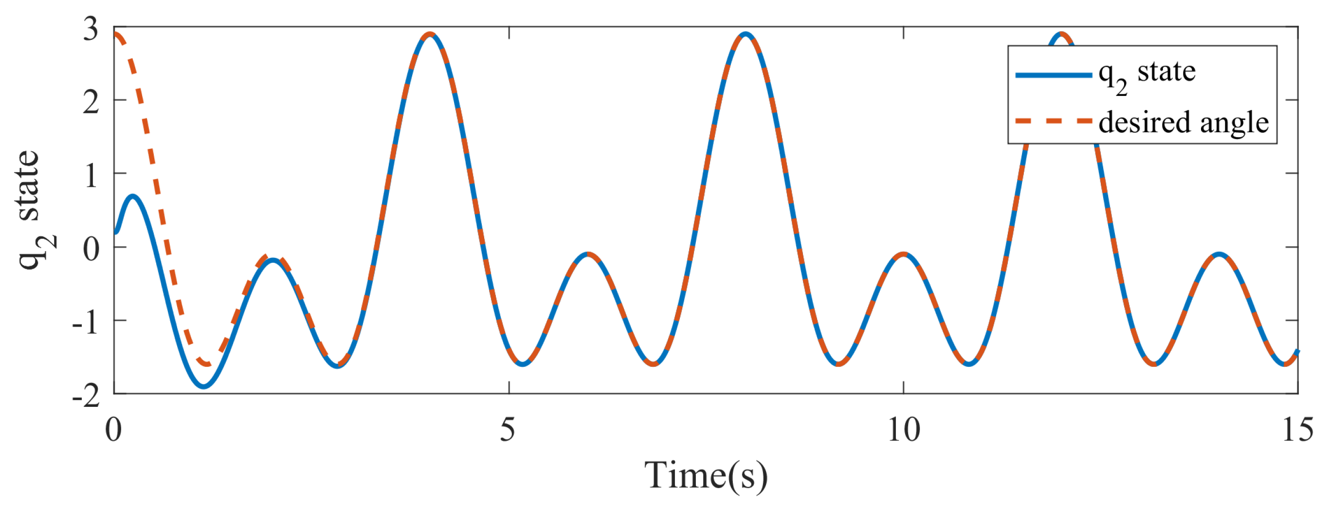
The proposed controller is implemented on the dynamical model of a two-link robot manipulator, as described earlier. The performance of the controller is evaluated by analyzing the states $q_a$ and $q_b$, which represent the angles of the first and second joints of the manipulator, respectively. Figure 7 and Figure 8 display the variations in the $q_a$ state and $q_b$ state over time. It is observed that the states $q_a$ and $q_b$ follow the desired trajectories, indicating that the controller effectively guides the manipulator to track the desired angles.

Furthermore, the settling time of the states $q_a$ and $q_b$ is finite, which indicates that the system reaches a stable state within a reasonable period. This demonstrates the fast convergence property of the proposed controller as it enables the system to achieve the desired angles efficiently and without undue delay. The successful tracking of the desired trajectories and the finite settling time of the states $q_a$ and $q_b$ are significant indicators of the effectiveness of the proposed controller. These results provide evidence of the controller’s ability to achieve accurate control and ensure the desired performance of the two-link robot manipulator.

In Figure 9 and Figure 10, the corresponding error signals for both states are depicted. The error signal represents the difference between the desired trajectory and the actual measured value of the system’s states. The error signals can be seen to converge to zero, indicating that the proposed controller successfully minimizes the discrepancy between the desired and actual states of the system. This demonstrates the controller’s ability to achieve accurate tracking of the desired trajectories for both states $q_a$ and $q_b$.

The convergence of the error signals to zero is a desirable characteristic in control systems as it signifies that the system is effectively following the desired behavior. It confirms that the controller is able to adjust the control inputs and guide the system toward the desired states, ensuring precise and reliable operation. The convergence of the error signals to zero in Figure 9 and Figure 10 provides strong evidence of the effectiveness of the proposed controller in achieving the desired control objective for the two-link robot manipulator. It demonstrates the controller’s ability to minimize errors and ensure accurate tracking of the desired states, enhancing the performance and stability of the system.

In Figure 11 and Figure 12, the control signals applied to the two-link robot manipulator are displayed. These control signals represent the inputs provided to the actuators of the manipulator to guide its motion and achieve the desired trajectories or positions.

Figure 11 shows the control signal applied to the first joint of the manipulator, denoted as $u_a$. This control signal is responsible for controlling the movement and positioning of the first link of the manipulator. The shape and behavior of the control signal can vary depending on the designed control strategy. It is designed to generate the necessary torque or force to drive the first joint and accurately track the desired trajectory.

Similarly, Figure 12 illustrates the control signal applied to the second joint of the manipulator, denoted as $u_b$. This control signal determines the motion and positioning of the second link of the manipulator. It is designed to provide the appropriate torque or force to the second joint, enabling precise control and tracking of the desired trajectory.

The control signals in Figure 11 and Figure 12 are generated by the proposed controller, taking into account the system dynamics, desired trajectories, and any uncertainties or disturbances present in the system. The control signals depicted in Figure 11 and Figure 12 demonstrate the ability of the proposed controller to generate appropriate inputs that guide the manipulator towards accurate and stable motion. These control signals play a crucial role in achieving the desired trajectories and ensuring the overall performance of the two-link robot manipulator.

Traditional control methods for robot manipulators often necessitate an exact model of the system, lacking the inherent robustness exhibited by the control approach itself. The PID control, despite its simplicity, encounters difficulties in effectively handling uncertainties and disturbances inherent in real-world scenarios [10,11,12]. On the other hand, SMC presents robustness against uncertainties, yet the issue of chattering—manifesting as oscillations in control input—diminishes its practical applicability [19,20,21]. Neural network control leverages neural networks for system learning, although its sensitivity to initial conditions can impact its performance [17,18].

In light of these considerations, the AFTN-SMC approach emerges as a solution to address these limitations. AFTN-SMC amalgamates sliding mode control, neural networks, and adaptability to effectively tackle the aforementioned challenges. Particularly noteworthy is its mitigation of chattering through dynamic adjustment of the sliding mode gain and harnessing neural networks to compensate for uncertainties. Consequently, AFTN-SMC yields refined control responses, attains elevated trajectory tracking accuracy, and reduces the exerted control efforts in comparison to conventional SMC. This research thus establishes AFTN-SMC as a more advanced alternative in the realm of robot manipulator control, offering improved performance under real-world complexities.

5. Conclusions

In conclusion, robot manipulators have become indispensable tools in environments where the safety and well-being of human operators are at risk. This research paper focused on designing an AFTN-SMC for a two-link robot manipulator with unknown dynamics and external disturbances. The proposed controller addressed the challenges of chattering and adaptability to time-varying system uncertainties. To approximate the unknown state dynamics, a radial basis function neural network (RBFNN) was employed. The MATLAB simulations demonstrated the successful implementation of the proposed controller.

The results showcased the effectiveness of the AFTN-SMC in achieving accurate tracking and stability, even in the presence of unknown dynamics and external disturbances. The chattering-free nature of the controller enhanced the smoothness of the manipulator’s motion, contributing to improved overall system performance. Additionally, the adaptive mechanism of the controller allowed for real-time adjustment and adaptation to time-varying uncertainties and parameter variations.

The incorporation of the RBFNN in the controller proved to be a valuable tool for approximating the unknown state dynamics, enabling accurate estimation and control of the manipulator’s behavior. This combination of adaptive sliding mode control and neural network approximation provided a robust and adaptive solution for handling significant uncertainties in real-time applications.

The research presented in this paper contributes to the advancement in control techniques for robot manipulators, particularly in situations where uncertainties and external disturbances are prevalent. The proposed AFTN-SMC controller, along with the RBFNN approximation, offers a practical approach for enhancing the performance, safety, and adaptability of robot manipulators in diverse industrial and automation applications. Future work may involve experimental validation and further optimization of the proposed control strategy for real-world implementation.