Detection of Weak Fault Signals in Power Grids Based on Single-Trap Resonance and Dissipative Chaotic Systems

Abstract

Aiming to solve the problem that the performance of classical time–frequency domain signal detection methods is severely degraded in highly noisy environments, a single-trap approximate model of the stochastic resonance of bistable systems is studied in this paper. This method improves the defects of the classical bistable stochastic resonance model that cause it to be inapplicable during non-periodic signal detection. Combining this method with the particle swarm optimization algorithm based on an attenuation factor and cross-correlation detection technology, detection experiments determining the impulse voltage fluctuation signals, motor speed fluctuation signals and low-frequency oscillation signals of a power system are conducted. The results show that the single-trap resonance model has good phase matching performance and noise cancellation abilities. Furthermore, combining it with two kinds of dissipative chaotic systems, a comprehensive frequency and amplitude detection experiment was carried out for multiple harmonic aliasing signals. The results show that the single-trap resonance model can achieve error-free detection of each harmonic frequency and high-precision detection of each harmonic amplitude in highly noisy environments. The research results will provide new ideas for the detection of various types of weak fault signals in power systems.

1. Introduction

Today’s power systems are constantly developing towards the creation of an integrated energy system and smart grid. With increasing amounts of new energy nodes, investments in power electronic equipment and the continuous improvement in voltage levels, power system electromagnetic environments are becoming increasingly complex, making power system fault signal detection increasingly difficult. At the same time, as the scale of the AC/DC hybrid power grid and the number of distributed micro-grids continue to increase, the difficulty of maintaining stable system operation also increases. Extreme weather and technical emergencies are more likely to affect the stable operation of the system. Emergency decision-making systems for microgrids and emergency energy management strategies for AC/DC microgrids have been studied in the literature [1,2]. Usually, these emergency management strategies are required to accurately identify the types and degrees of system faults in order to achieve effectiveness. However, the electromagnetic environment in faulty large-scale power grids is extremely complex, and many fault feature signals are engulfed in strong background noise. Accurately extracting fault feature signals poses great difficulties. Among traditional time–frequency domain signal processing methods, such as the discrete Fourier transform, modal decomposition, matrix beams, singular value decomposition, etc. [3,4,5,6], the lowest detectable environmental signal-to-noise ratio is only −20 dB. Therefore, an efficient and accurate weak signal detection method is urgently needed in the fields of harmonic monitoring, low-frequency oscillation identification, motor fault diagnosis and fault location.

An inter-harmonic detection method based on the SST (synchrosqueezing wavelet transform) was proposed in the literature [6], realizing mixed harmonic signal detection with a relatively low number of errors in environments with a sufficient signal-to-noise ratio. However, in noisy environments with a negative signal-to-noise ratio, the detection accuracy of this method is significantly reduced. A power system harmonic detection method based on the fractional wavelet transform was proposed in the literature [7]. In environments with less noise, the relative error is small and weak harmonic amplitude detection is realized, improving the detection accuracy to a certain extent. However, when processing the signal itself, signal details will inevitably be lost, eliminating detection errors will become difficult and signal details will gradually increase with an increase in noise; thus, it is difficult to apply in highly noisy environments.

A low-frequency oscillation identification method based on signal correlation was proposed in the literature [8], which can identify and detect parameters such as the frequency, amplitude, attenuation coefficient and start–stop time of the low-frequency oscillation component’s dynamic process; however, this method is limited in that it produces a large error. A power system transmission line fault classification method using wavelet detail coefficients was also proposed in the literature [9]. This algorithm relies on accurately distinguishing wavelet coefficients, so there are strict requirements for the selection of wavelet bases, and it is usually very difficult to select wavelet bases for specific signals. However, decomposing too many layers with the wavelet transform will lead to a loss of signal detail. In the future, the scale of integrated energy systems and the voltage level will continue to increase and this method will have limitations.

R Benzi proposed a principle in [10] to detect signals below the instrument’s recognizable threshold; if Gaussian noise is added to the sub-threshold (that is, non-measurable) signal, the sub-threshold signal can be turned into a recognizable signal. The detection area and the noise are removed after detection, and the removed noise energy is converted into the energy of the sub-threshold signal, which can expand the detection range of the instrument four-fold. Due to the existence of random noise, this phenomenon was called stochastic resonance. Since the concept of stochastic resonance was proposed, researchers in various fields have been studying the application of the stochastic resonance principle in weak signal detection. Gammaitoni L proposed a principle in [11] that under adiabatic approximation conditions, stochastic resonance can occur in bistable systems. This can be used to detect the frequency components of weak signals. Gang H analyzed the periodic forced Fokker–Planck equation in [12] and concluded that the adiabatic approximation condition is only valid under the condition of low-frequency, small-parameter signals, and the adiabatic approximation model of stochastic resonance cannot be directly applied to high-frequency, large-parameter signals. In [13,14,15], stochastic resonance is processed via parameter normalization, scaling and subsampling so that the stochastic resonance principle can be applied to high-frequency and large-parameter signals. In the wake of this advancement, the stochastic resonance principle has been applied in various fields.

At the same time, with the development of the stochastic resonance principle, the application of various chaotic systems for weak signal detection is also increasing on a daily basis. According to the related chaos theory [16,17], it was found that a chaotic oscillator has extremely high sensitivity to specific weak signals [18] and has strong immunity to random noise [19]. When a weak signal with the same frequency as the driving force is input into a chaotic system in a critical state, it will cause a phase transition of the system [20]. This characteristic of chaotic systems gives them a unique advantage in the field of weak signal detection. Non-dissipative chaotic systems such as Duffing and van der Pol systems are the most widely developed and applied. Duffing and van der Pol systems were used, respectively, to realize the detection of weak signals in [21,22,23,24], but these two types of systems are different to other non-dissipative chaotic systems. Dissipative chaotic systems are not particularly adept at anti-noise determination, and their detection accuracy needs to be further improved.

In this paper, for the first time, two dissipative chaotic systems (Chen and Yang systems) are combined with the principle of single-trap stochastic resonance and applied for the detection of weak harmonic signals in power systems. Impulse voltage fluctuation signal, motor speed fluctuation signal and power system low-frequency oscillation signal detection experiments based on single-trap stochastic resonance are designed. The experimental results show that for non-periodic signals, the single-trap stochastic resonance detection method can maintain the signal phase to a high extent. Matching eliminates the nonlinear distortion generated by random resonance; a cascaded stochastic resonance system is designed, and through various simulation experiments, it is found that the cascaded stochastic resonance system has the advantage of step-by-step detection effect optimization. A power system harmonic detection experiment is designed, using a system bifurcation diagram, a phase trajectory diagram, the attractor distribution and the state variable time trajectory to analyze the Yang and Chen systems. Corresponding weak harmonic amplitude detection is achieved according to the characteristics of each system algorithm; an amplitude detection test is carried out on the harmonic components detected based on the stochastic resonance principle. The results show that dissipative chaotic systems have significant advantages in the detection of weak harmonics in power systems and have great development prospects. The results of this paper provide a new method and research experience for the accurate detection of various weak fault signals in power systems with a strong noise background.

This paper is organized as follows: The classical stochastic resonance principle and the single-trap approximate model of stochastic resonance are introduced in Section 2. The reasons behind the stochastic resonance principle producing nonlinear distortion are analyzed, a stochastic resonance follower system that can eliminate nonlinear distortion is designed, and a system model and a cascaded stochastic resonance model for stochastic resonance detection in engineering signals are presented. In Section 3, tools such as bifurcation diagrams, phase diagrams, the attractor distribution and the time history of system state variables are used to analyze the characteristics and performance of the Yang and Chen systems, and a dissipative chaotic system is designed for weak harmonic amplitude detection. In Section 4, the single-trap stochastic resonance model and the cascaded model are used to test the harmonic simulation signals, voltage fluctuation signals, motor speed signals and low-frequency oscillation signals of the power system, and the Yang and Chen systems are used to analyze the amplitude of the weak harmonic signal. The experimental results and method efficiency are analyzed and compared. In Section 5, some concluding observations are stated.

2. Detection Principle Based on Stochastic Resonance

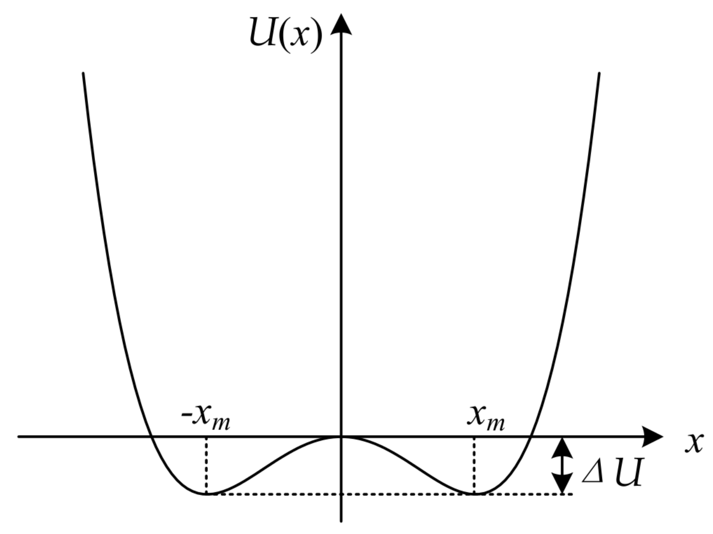
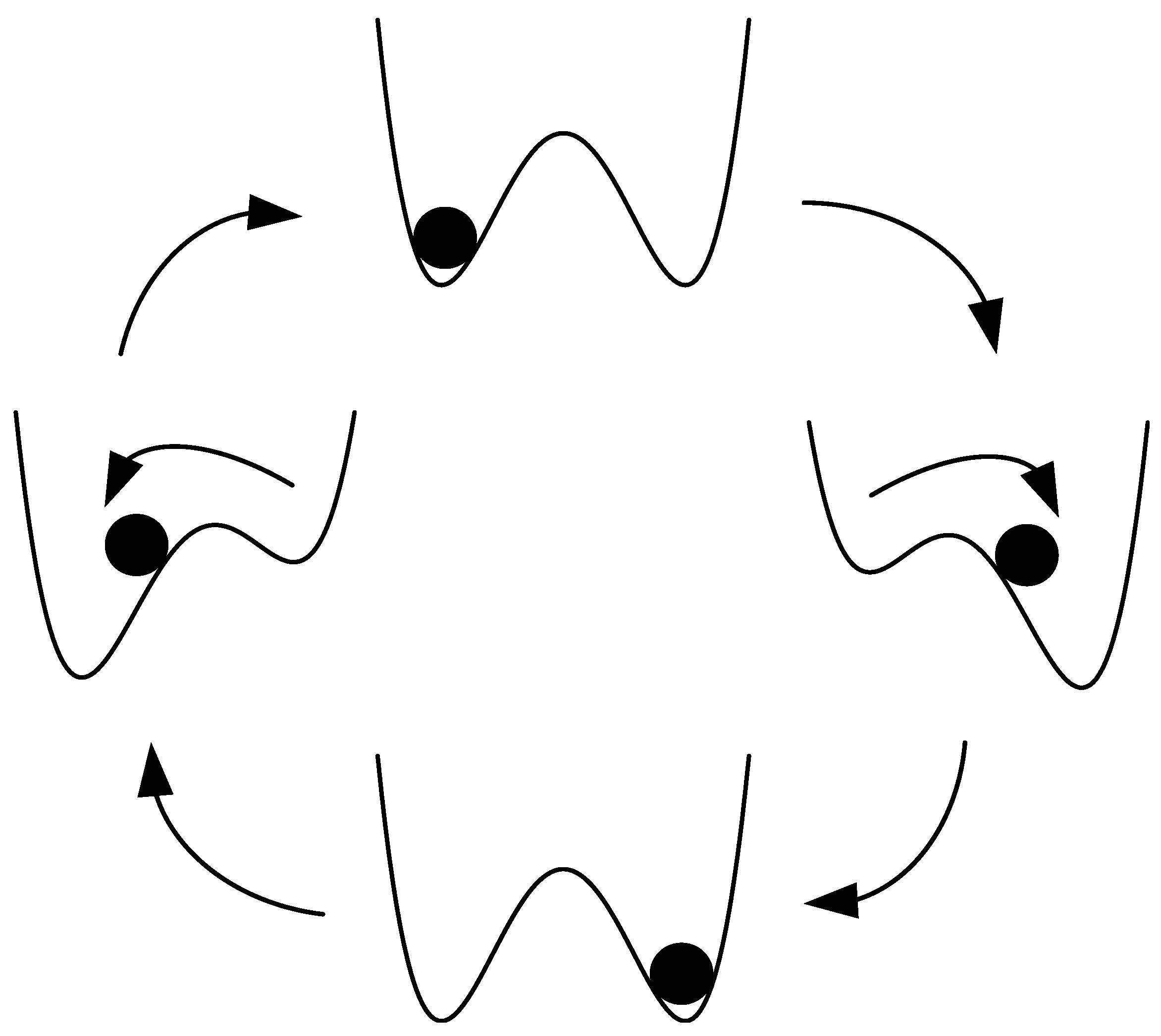
2.1. Fundamentals of Stochastic Resonance

When a nonlinear system achieves a certain synergistic effect with the periodic signal and random noise, the system’s nonlinear effect is used to convert the energy of part of the random noise into the energy of the periodic signal, weakening the noise, enhancing the periodic signal and improving the signal-to-noise ratio of the output signal, a phenomenon known as the stochastic resonance phenomenon. The classical nonlinear model that describes the stochastic resonance phenomenon is the Langevin equation with a double potential well [25]:

$$\frac{dx}{dt}=-U^{{}^{\prime }}\left(x\right)$$

(1)

In this formula, $U\left(x\right)$ is the potential function of the bistable system, which has a quartic polynomial structure [26]:

$$U\left(x\right)=-\frac{1}{2}a{x}^2+\frac{1}{4}b{x}^4$$

(2)

In this formula, $a>0$ and $b>0$ are the parameters of the bistable system. The potential function curve of the bistable system is shown in Figure 1.

It can be seen from Figure 1 that the bistable system has two symmetrical stable points $\pm x_m$, $x_m$, which have the following relationship with system parameters a and b:

$$x_m=\sqrt{a/b}$$

(3)

$x_U=0$ is an unstable point of the bistable system, and the potential difference $\mathsf{\Delta }U$ between the stable point and the unstable point is called the potential barrier.

$$\mathsf{\Delta }U=a^2/4b$$

(4)

When the drive signal

$$s\left(t\right)=Asin\left(2\pi ·f_0·t\right)$$

and Gaussian white noise $n\left(t\right)$ are used as the input of the bistable system, the Langevin equation is [27]:

$$\frac{dx}{dt}=ax-b{x}^3+Asin\left(2\pi ·f_0·t\right)+n\left(t\right)$$

(5)

where $n\left(t\right)$ satisfies:

$$〈n\left(t\right)〉=0$$

(6)

$$〈n\left(t\right)·n\left(t^{{}^{\prime }}\right)〉=2D\delta \left(t-t^{{}^{\prime }}\right)$$

(7)

In this formula, D is the noise intensity and $\delta$ is the unit impulse signal. It can be seen from Formula (1) that after the drive signal and noise are input into the system, the potential function of the bistable system is modulated by the input signal, becoming:

$$U_s\left(x\right)=-\frac{1}{2}a{x}^2+\frac{1}{4}b{x}^4-x\left(Asin\left(2\pi f_{0}t\right)+n\left(t\right)\right)$$

(8)

It can be seen from Formula (6) that the input signal will have a periodic impact on the system potential function, so that the system potential function will be reversed and distorted according to the period of the driving signal. The output of the system is equivalent to the motion of the proton in the potential function; thus, the system output x is the trajectory of the proton and $x^{{}^{\prime }}$ is the speed of the proton. When the initial position of the proton is $x_0>0$, the system tends to the positive stable point $+x_m$; when the initial position of the proton is $x_0<0$, the system tends to the negative stable point $-x_m$; and when the position is $t\to \infty$, the system tends to the stable state on an infinite basis. A special case is when the proton is at the initial position $x_0=0$; the proton is at the unstable point $x_U=0$ and any disturbance will make the proton fall into the potential well where the two stable points are located; that is, the system will tend to a stable state after being disturbed.

When $A\ne 0$ and $D\ne 0$, the noise $n\left(t\right)$ is introduced, and as D continues to increase to a certain value, the noise, the periodic drive signal and the bistable system achieve a synergistic effect. The protons are excited by the noise energy to overcome the potential barrier between the two stable points; the transition frequency depends on the frequency of the potential function flipping and twisting. Thus, the energy of the noise will accompany the proton transition, showing an output state with the same frequency as the periodic driving signal, and thus the randomness of the noise is suppressed and transformed into a periodic output, which enhances the periodic signal and improves the output signal-to-noise ratio. The proton stochastic resonance transition model of a nonlinear system is shown in Figure 2.

2.2. A Single-Trap Approximate Model of Stochastic Resonance

When the input periodic signal amplitude A satisfies the following relationship [25]:

$$A>\sqrt{\frac{4a^3}{27b}}$$

(9)

the potential function of the bistable system will lose the double potential well shape during the twisting process; thus, the system output presents monostable characteristics in a large range.

In addition, when the mixed input of periodic signal and noise is not enough to make the proton jump out of the potential well and jump between the two potential wells, the output of the system can only oscillate in one potential well.

In the past, scholars have always believed that the stochastic resonance’s enhancement effect can only occur in the oscillation process of the double-well transition. A single-trap approximate model of stochastic resonance was proposed in [28].

This model can also amplify the input periodic signal in a bistable system under the single-trap approximate condition.

The monostable approximation is applied to the bistable system; that is, the protons only exhibit simple harmonic motion around the stable points $+x_m$ or $-x_m$ in the potential well in a single potential well. Then, the potential function $U_s\left(x\right)$ of the bistable system under the single-well approximation can be described $U_{ss}\left(x\right)$:

$$U_{ss}\left(x\right)=U_s^{{}^{\prime \prime }}\left(x_s\right)·\frac{{\left(x-x_s\right)}^2}{2}$$

(10)

It can be seen from Formula (8) that when a mixed signal is input, it satisfies:

$$U_s^{{}^{\prime }}\left(x\right)=-ax+b{x}^3-s\left(t\right)-n\left(t\right)$$

(11)

Equation (11) is a stochastic differential equation, and the solution of the equation is usually not unique. In order to analyze the steady-state output characteristics of the system, the steady-state solution of the equation is obtained according to the differential equation analytical solution method:

$$x=-U_s^{{}^{\prime \prime }}\left(x_s\right)·\left(x-x_s\right)+C\left(t\right)$$

(12)

Equation (12) is the single-trap approximate model of a bistable system. At this time, the probability density $\rho \left(x,t\right)$ of the system output satisfies the Fokker–Planck equation [29]:

$$\frac{\partial \rho \left(x,t\right)}{\partial t}=-U_s^{{}^{\prime \prime }}\left(x_s\right)\frac{\partial }{\partial x}\left[\left(x-x_s\right)\rho \left(x,t\right)\right]+D_F\frac{{\partial }^2}{\partial x^2}\rho \left(x,t\right)$$

(13)

In this formula, $D_F$ is the diffusion coefficient, and the equation describes the probability density function of the velocity of a proton under the action of random force. The minimum non-zero eigenvalue ${\lambda }_{min}$ of the Fokker–Planck equation is:

$${\lambda }_{min}=U_s^{{}^{\prime \prime }}\left(x_s\right)$$

(14)

${\lambda }_{min}$ directly determines the speed of the system response; if the system response is too slow, there will be a significant phase difference between the system output and the system input; that is, nonlinear distortion. If the response speed of the system is too fast, the transition process of random noise energy to sinusoidal state energy in the system is too short and the noise energy cannot be properly converted into signal energy; the system noise output will increase proportionally.

In the single-trap approximate model, low-frequency, small-parameter signal inputs are usually considered, so if $x_s\approx \pm x_m=\pm \sqrt{a/b}$, then:

$${\lambda }_{min}=2a$$

(15)

It can be seen from Formula (15) that the parameter a of the bistable system determines the speed of the system response, so the choice of the parameter a determines the single-trap approximate model detection performance.

Due to the single-trap approximate model, the phase match between the input and output is considered; thus, the model is applicable to both non-periodic and periodic signals and the key problem is how to solve the distortion of the model.

2.3. Nonlinear Distortion and Restoration of Stochastic Resonance

Through the above analysis, it is concluded that when there is no noise input or the noise is small, protons exhibit similar simple harmonic motion around the stable points $+x_m$ or $-x_m$ in a single potential well of a bistable system. In engineering, the noise intensity can be controlled by controlling the sampling rate, so the actual signal can be re-sampled to obtain a noise intensity that can achieve single-trap resonance. When the noise intensity is small or the noise intensity is zero, the kinetic energy provided by the noise to the proton is very small, and thus the velocity of the proton will be very small. Consider $x^{{}^{\prime }}=0$, then the approximate form of the Langevin equation is:

$$0=ax-b{x}^3+Asin\left(2\pi f_{0}t\right)+n\left(t\right)$$

(16)

Since there are random items in the Langevin equation, it is necessary to discuss the expected distortion degree of the system output from the perspective of statistical averages. The statistical average of the left and right side of Equation (16) is taken to obtain:

$$0=ax-b{x}^3+Asin\left(2\pi f_{0}t\right)$$

(17)

Analyzing the time history of the proton, the two sides of Formula (17) are, respectively, derived with respect to time t, and the results of the derivation are transposed and arranged to obtain:

$$\frac{dx}{dt}=\frac{1}{-a+3b{x}^2\left(t\right)}·s^{{}^{\prime }}\left(t\right)$$

(18)

It can be seen from Formula (18) that the first-order derivative of the system output x is not equal to the first-order derivative of the input signal $s\left(t\right)$ and there is a nonlinear coefficient term, indicating that there is nonlinear distortion between the time history of the proton and the time history of the input signal, which will lead to a phase deviation between the output signal and the input signal.

Transposing Formula (17) will obtain:

$$-ax+b{x}^3=Asin\left(2\pi f_{0}t\right)$$

(19)

The right side of Equation (19) is the input periodic target signal, and the left side can be regarded as the output signal of a certain system. When the input is the output signal x of a bistable system, the output signal and the periodic input signal phase of the bistable system satisfy the matching relationship.

Therefore, the system is defined as a follower system $Q\left(u\right)$ of bistable stochastic resonance, and its function is to eliminate the distortion caused by the nonlinear process of stochastic resonance in the input signal. The system model with input u is:

$$Q\left(u\right)=-au+b{u}^3$$

(20)

Equation (20) is the follower system of a bistable stochastic resonance system with parameters a and b, and the system input is the output of the stochastic resonance system, that is, $Q\left(u\right)$ and the stochastic resonance system is cascaded.

2.4. Stochastic Resonance Frequency Detection Model for Engineering Signals

The stochastic resonance model discussed above is a small-parameter, low-frequency model under the adiabatic approximation condition, which requires the frequency of the periodic driving signal to be much lower than 1 Hz and the amplitude to be much smaller than 1 p.u. Most power system engineering signals do not satisfy the low-frequency small-parameter model conditions. Therefore, it is necessary to improve the stochastic resonance model or to preprocess the engineering signal to meet the low-frequency and small-parameter conditions.

The idea of mathematical normalization can be used to normalize the stochastic resonance model. After processing, different values can be set through system parameter a to realize the frequency normalization of high-frequency signals [30]. However, the parameter adjustable range of this method is limited, and when the value of a is too large, this often leads to divergence in the iterative solution of the Langevin equation. Thus, in this paper, a signal subsampling method with stronger stability and applicability is adopted [31].

The sampling frequency of the original signal is $f_s$, and the time interval of sampling points is $T_s$. First, the scaling factor R of re-sampling is determined to obtain the re-sampling frequency $f_{sr}$:

$$f_{sr}=\frac{f_s}{R}$$

(21)

Retaining the same number of signal sampling points, the time interval of each sampling point after re-sampling becomes:

$$T_{sr}=\frac{R}{f_s}=R·T_s$$

(22)

The iterative step size h of the Runge–Kutta method for solving the Langevin equation is:

$$h=\frac{1}{f_{sr}}$$

(23)

From Formula (22), it can be seen that the time interval of signal sampling points after re-sampling is R times that of the original, which is equivalent to reducing the frequency of the signal to the original $1/R$. Thus, it is only necessary to select an appropriate R to achieve stochastic resonance of high-frequency signal detection. In practical engineering, the frequency component of the detected signal is usually unknown, so it is not feasible to use the signal-to-noise ratio as the evaluation index of the stochastic resonance detection effect. The cross-correlation coefficient between the input signal and the output signal of the bistable system reflects the phase matching degree of the input and output signals and has no requirement for the signal components. It is an ideal parameter for evaluating the effect of stochastic resonance detection in practical engineering. Taking the cross-correlation coefficient between the input and output of the bistable system as the objective function of system parameter optimization, various optimization algorithms can be used to find the system parameters a and b that lead to the best detection effect. The algorithm model used in paper [27] is shown in Figure 3.

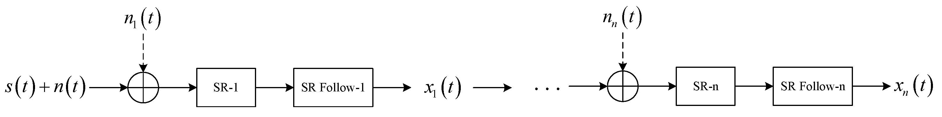
2.5. Cascaded Stochastic Resonance Frequency Detection Model

Referring to the cascading principle of the filter, the stochastic resonance system is cascaded in multiple levels and the random noise is weakened or transformed step by step, and thus the target signal and the output signal-to-noise ratio are improved step by step. If the target signal is a weak periodic signal and the purpose of processing is to enhance the periodic signal, an appropriate amount of Gaussian white noise can be artificially added to the input of each stochastic resonance system to provide energy to enhance the periodic signal. The cascaded stochastic resonance model has an improved detection performance and more flexible scalability. The multi-layer cascaded stochastic resonance detection model is

$$\left\{\begin{array}{c}{x}_1^{{}^{\prime }}=a_1{x}_1-b_1{x}_1^3+Asin\left(2\pi ·f_0·t\right)+n\left(t\right)\hfill \\ x_2^{{}^{\prime }}=a_2{x}_2-b_2{x}_2^3+x_1\left(t\right)\hfill \end{array}\right.$$

(24)

The model structure is shown in Figure 4.

3. Periodic Amplitude Detection of Dissipative Chaotic Systems

There is no forced periodic driving force with explicit time in dissipative chaotic systems, so it is impossible for the system to reach a resonance state by adjusting the forced control of system parameters. The non-resonance parameter control method proposed in [32] is used to control the dissipative chaotic system, and the amplitude of the periodic weak signal is detected by observing the phase transition of the system. The study found that compared to non-dissipative chaotic systems such as the Duffing system, dissipative chaotic systems have stronger noise resistance and detection sensitivity. The Yang and Chen systems have distinct periodic signal detection signs. Two kinds of dissipative chaotic systems are used in this paper; they can accurately extract the amplitude of weak periodic signals.

3.1. Yang System

The non-resonance parametric control model of the Yang system [32] is:

$$\left\{\begin{array}{c}\frac{dx}{dt}=a\left(y-x\right)\hfill \\ \\ \frac{dy}{dt}=cx-xz\hfill \\ \\ \frac{dz}{dt}=xy-bz\left(1+fcos\omega t\right)\hfill \end{array}\right.$$

(25)

In this formula, x, y and z are the state variables of the system, and a, b and c are dimensionless system parameters. $1+fcos\omega t$ is the control signal and $\omega$ is the angular frequency of the periodic component of the control signal.

Under the condition that the system parameters are set to $\left(a,b,c\right)=\left(35,3,35\right)$ and the initial values are set to $\left(x_0,y_0,z_0\right)=\left(1.15,3.5,3.3\right)$, the bifurcation diagram of the system state variables x and z changing with the control signal amplitude f is shown in Figure 5.

It can be seen from Figure 5 that the Yang system does not have a large-period state similar to the Duffing system and the system state is composed of countless different chaotic states; however, the bifurcation diagrams of the system state variables x and z all have a flat envelope, and the amplitude range of the flat area corresponding to the periodic component of the control signal is about 0.57∼0.75. The flat envelope of the state variable x is mostly negative, and the non-flat envelope is randomly distributed with a large number of positive and negative values. The flat envelope values of the state variable z are all negative, and the non-flat envelope is randomly distributed with a large number of positive values. Therefore, the Yang system has a “chaos-to-chaos” phase transition with obvious differences between the phase diagram and the distribution of attractors; the Yang system can be used to detect weak harmonic signals. According to the dichotomy test, the phase change critical value of the amplitude of the periodic component of the Yang system control signal is 0.5705276. Thus, the Yang system can generally provide an amplitude detection accuracy of ${10}^{-7}$ in a noise-free environment; that is, the Yang system can control the amplitude of the signal’s periodic component. When the value is 0.5705277, it has a phase trajectory that is significantly different from the critical state. The Yang system chaotic critical state and the phase trajectory and attractor distribution after entering the flat envelope are shown in Figure 6 and Figure 7, where the red dots in the figures are attractors.

3.2. Chen System

The non-resonant parameter control model of the Chen system [32] is:

$$\left\{\begin{array}{c}\frac{dx}{dt}=\alpha \left(y-x\right)\hfill \\ \\ \frac{dy}{dt}=\gamma \left(x+y\right)-xz-\alpha x\hfill \\ \\ \frac{dz}{dt}=xy-\beta z\left(1+fcos\omega t\right)\hfill \end{array}\right.$$

(26)

In this formula, x, y and z are the state variables of the system, and $\alpha$, $\beta$ and $\gamma$ are dimensionless system parameters. $1+fcos\omega t$ is the control signal and $\omega$ is the angular frequency of the periodic component of the control signal.

Under the condition that the system parameters are set as $\left(\alpha ,\beta ,\gamma \right)=\left(38,3,21\right)$ and the initial values are set as $\left(x_0,y_0,z_0\right)=\left(1,1,1\right)$, the bifurcation diagram of the system state variables x and z changing with the control signal amplitude f is shown in Figure 8.

It can be seen from Figure 8 that the Chen system does not have a large-period state and the system state is composed of countless different chaotic states. The bifurcation diagram of the system state variables x and z has a flat envelope area. The difference from the Yang system is that the flat envelope of the Chen system is the persistent region and the flat envelope of the Yang system is the locality region. The threshold value of the control signal’s periodic component for the Chen system to enter the flat envelope region is (0.65,0.75). The critical amplitude of the control signal’s periodic component for the Chen system is 0.7014001824, which is determined through a dichotomy test. Therefore, the Chen system can generally provide a ${10}^{-10}$ amplitude detection accuracy in a noise-free environment; that is, the Chen system has a phase trajectory that is significantly different to the critical state when the amplitude of the control signal’s periodic component is 0.7014001825. The chaotic critical state of the Chen system and the phase trajectory and attractor distribution after entering the flat envelope are shown in Figure 9 and Figure 10, where the red dots in the figure are attractors.

Comparing Figure 9 and Figure 10, it can be seen that after the system bifurcates and enters the flat envelope stage, the fixed point at which the system attractors accumulate changes from the second quadrant of the phase space in the critical state to the first quadrant of the phase space. By observing the time histories of the state variables x and z, the coordinates of the fixed point in the system’s critical state are (−3.86, 4.99), and the coordinates of the fixed point after the bifurcation enters the flat envelope region are (3.86, 4.99). The coordinates of the fixed point in different chaotic states are clearly different, so this feature of the Chen system has high sensitivity and reliability as a judgment index for weak harmonic signal detection.

4. Simulation and Experiment

4.1. Steady State Harmonic Amplitude Detection Simulation

In order to compare the chaos method with the classical time–frequency domain method, the weak harmonic signal of a power system from the literature is used ($x\left(t\right)=sin\left(\omega t\right)+0.15sin\left(2.2\omega t\right)+0.25sin\left(3\omega t\right)+0.2sin\left(5\omega t\right)+0.1sin\left(7\omega t\right)$) for simulation. The angular frequency $\omega =2\pi f$ and the fundamental frequency component frequency $f=50\mathrm{Hz}$.

The simulation was conducted in a noisy environment with an SNR of 20 dB, −20 dB, −60 dB and −100 dB, respectively. The noise form was Gaussian white noise. The noise intensity D is determined by the SNR and signal variance Var(x) [33]:

$$D=\sqrt{\frac{\mathrm{Var}\left(x\right)}{{10}^{SNR/10}}}$$

(27)

In the −20 dB and −30 dB SNR environments, the single-stage single-trap stochastic resonance model and the two-stage cascaded single-trap stochastic resonance model were used to detect the harmonic signal frequency, respectively. The spectrum image of the restored system output signal is shown in Figure 11. The frequency detection data are shown in

Table 1. Single-well stochastic resonance harmonic frequency detection results.

Harmonic Order	Theoretical Value (Hz)	Detected Value (Hz)	SR Error (%)	VMD Error (%)	EEMD Error (%)	SST Error (%)
(a) SNR = −20 dB
1	50	50	0	0.02	0.11	0
2.2	110	110	0	0.07	0.06	0.03
3	150	150	0	0.04	0.15	0.08
5	250	250	0	0.12	0.13	0.08
7	350	350	0	0.17	0.19	0.11
(b) SNR = −30 dB
1	50	50	0	0.12	0.32	0.07
2.2	110	110	0	0.17	0.43	0.11
3	150	150	0	0.23	0.39	0.19
5	250	250	0	0.27	0.51	0.28
7	350	350	0	0.43	0.71	0.29

.

It can be seen from Figure 11 that each component of the harmonic signal has been enhanced, the spectrum has been significantly improved, the output signal-to-noise ratio has been improved and the detection effect of the cascaded system has been significantly improved. Compared with the single-stage system, the noise has been further suppressed. Harmonics at all levels are further enhanced.

From the comparison of the data in Table 1, it can be seen that the single-trap stochastic resonance method can detect the frequency of each harmonic component with zero error in a highly noisy environment. However, traditional time–frequency domain filtering algorithms lead to some frequency detection errors. In order to determine the amplitude of each harmonic component accurately, it is necessary to use the chaotic system.

The system parameters and initial system values of the Yang and Chen systems were maintained, the forced driving force frequency of the system or the periodic component of the control signal were set as the frequency of each harmonic signal component, the forced driving force was found through the dichotomy test threshold for the periodic component of the force or control signal and the system was set to a critical state. In the noise environments of 20 dB, −20 dB, −60 dB and −100 dB, the amplitude of each harmonic component was detected, respectively, and the detected value and relative error are shown in

Table 2. Steady-state harmonic amplitude detection results of the chaotic system.

Harmonic Order	Actual Value/p.u.	Detection Value/p.u.	Relative Error/%
(a) SNR = 20 dB, Yang system
1	1.0	1.0	0
2.2	0.15	0.15	0
3	0.25	0.25	0
5	0.2	0.2	0
7	0.1	0.1	0
(b) SNR = 20 dB, Chen system
1	1.0	1.0	0
2.2	0.15	0.15	0
3	0.25	0.25	0
5	0.2	0.2	0
7	0.1	0.1	0
(c) SNR = −20 dB, Yang system
1	1.0	1.0	0
2.2	0.15	0.15	0
3	0.2498	0.25	0
5	0.2	0.2	0
7	0.1	0.1	0
(d) SNR = −20 dB, Chen system
1	1.0	1.0	0
2.2	0.15	0.15	0
3	0.25	0.25	0
5	0.2	0.2	0
7	0.1	0.1	0
(e) SNR = −60 dB, Yang system
1	1.0	1.0	0
2.2	0.15	0.15	0
3	0.25	0.25	0
5	0.2	0.2	0
7	0.1	0.1	0
(f) SNR = −60dB, Chen system
1	1.0	1.0000122	0.00122
2.2	0.15	0.1499985	0.001
3	0.25	0.25	0
5	0.2	0.2000036	0.0018
7	0.1	0.0999898	0.0102
(g) SNR = −100 dB, Yang system
1	1.0	1.00207	0.207
2.2	0.15	0.14983	0.113
3	0.2498	0.25127	0.508
5	0.2	0.19972	0.14
7	0.1	0.09981	0.19
(h) SNR = −100 dB, Chen system
1	1.0	1.0204031	2.0403
2.2	0.15	0.1517132	1.1421
3	0.25	0.2449147	2.0341
5	0.2	0.2040105	2.0053
7	0.1	0.0966392	3.3608

.

It can be seen from Table 2 that both kinds of chaotic systems can realize the undifferentiated detection of each harmonic component’s amplitude in the SNR environment of 20 dB. Compared with time–frequency domain methods such as the empirical wavelet transform, the chaos detection method has a greatly improved detection accuracy. Comparing the detection results in −20 dB, −60 dB and −100 dB SNR environments, it is concluded that the detection sensitivity of the Chen system is ${10}^{-7}$ and the detection sensitivity of the Yang system is ${10}^{-5}$; the Yang system has the strongest anti-noise performance, followed by the Chen system. Regardless of the detection sensitivity or anti-noise performance, the chaos detection method is much more sensitive than the classical time–frequency domain detection method.

4.2. Detection Experiment of DC Transmission Line Voltage Fluctuation

In this experiment, the voltage monitoring data of a transmission line in a DC transmission project in China were used as the experimental signals. The normal operating voltage of this line was reduced to 1.03 p.u., and the monitoring center detected two large fluctuations in the line voltage due to disturbances during a certain period of time. The bistable system parameters a and b and the re-sampling compression ratio R were used as optimization parameters, and the cross-correlation coefficient between the original signal and the recovery system output signal was used as the fitness function of the particle swarm algorithm. An algorithm-based adaptive single-trap stochastic resonance method was used for detection. After iterative optimization, the optimal system parameters were a = 0.12 and b = 9.76, the optimal sub-sampling compression ratio was R = 80.3 and the input–output correlation coefficient corresponding to the optimal parameters was 0.98826. The experimental results are shown in Figure 12.

It can be seen from Figure 12 that the original signal is processed by using the stochastic resonance of the bistable system to produce phase distortion, and then processed by the following system. The waveform effect is good, the output signal noise of the two-stage cascaded system is further suppressed and the signal-to-noise ratio of the output signal noise has improved. Compared to the test data from the test center, the results of the single-stage system are shown in

Table 3. Comparison of detection data from a single-stage random resonance system for voltage fluctuation in a DC transmission line.

	Detection Value/s		Monitoring Center Data Value/s
	First	Second	First	Second
(a) Disturbance moment
Experimental data	0.2992 (+)	1.6021 (+)	0.3 (+)	1.6 (+)
	0.4998 (−)	1.8968 (−)	0.5 (−)	1.9 (−)
	Detection Value/p.u.		Monitoring Center Data Value/p.u.
	First	Second	First	Second
(b) Voltage fluctuation
Experimental data	0.3504 (+)	0.1849 (+)	0.348 (+)	0.186 (+)
	0.1129 (−)	0.1062 (−)	0.112 (−)	0.107 (−)

and the results of the two-stage cascade system are shown in

Table 4. Comparison of detection data from a DC transmission line voltage fluctuation secondary cascade random resonance system.

	Detection Value/s		Monitoring Center Data Value/s
	First	Second	First	Second
(a) Disturbance moment
Experimental data	0.2992 (+)	1.6007 (+)	0.3 (+)	1.6 (+)
	0.5001 (−)	1.8993 (−)	0.5 (−)	1.9 (−)
	Detection Value/p.u.		Monitoring Center Data Value/p.u.
	First	Second	First	Second
(b) Voltage fluctuation
Experimental data	0.3491 (+)	0.1853 (+)	0.348 (+)	0.186 (+)
	0.1121 (−)	0.1072 (−)	0.112 (−)	0.107 (−)

.

According to the data in Table 3, the relative error of the first disturbance detection is 0.83% (+), 0.04% (−), and the relative error of the voltage fluctuation detection is 0.69% (+), 0.80% (−). The relative error of secondary disturbance moment detection is 0.13% (+), 0.17% (−), and the relative error of voltage fluctuation detection is 0.59% (+), 0.75% (−). According to the data in Table 4, the relative error of first disturbance detection is 0.27% (+), 0.02% (−), and the relative error of voltage fluctuation detection is 0.32% (+), 0.09% (−). The relative error of secondary disturbance detection is 0.04% (+), 0.04% (−), and the relative error of voltage fluctuation detection is 0.38% (+), 0.19% (−). It can be seen that the bistable system single-trap approximate stochastic resonance model has a good effect when the system parameters are appropriately selected, and the system cascade can further optimize the detection effect.

4.3. Motor Speed Sensor Signal Detection Experiment

The rotational speed of the generator rotor is an important parameter in the analysis of the safety and stability of a power system. Abnormal fluctuations in the rotor rotational speed should be detected in time and the cause should be checked. The difference curve between the motor rotational speed and the rated rotational speed collected by the motor control center of the unit in a certain period of time is determined. As an experimental signal, the rotational speed is calculated as a per unit value, with 100 r/s as the reference value. Due to performance limitations of the inertial sensor that monitors the rotational speed and the strong magnetic interference of the generator’s operating environment, the original signal data are engulfed in strong background noise. The adaptive single-trap stochastic resonance method based on the particle swarm algorithm was used to test the collected rotational speed signal. After iterative optimization, the optimal system parameters were a = 0.611 and b = 0.032, the optimal sub-sampling compression ratio was R = 7.48 and the input–output correlation coefficient corresponding to the optimal parameters was 0.99848. The experimental results are shown in Figure 13.

It can be seen from Figure 13 that the original signal is amplified after being processed by the stochastic resonance of the bistable system, but at the same time, phase distortion is generated. The signal noise is further suppressed and the output signal-to-noise ratio is further improved.

4.4. Low Frequency Oscillation Signal Detection Experiment

The low-frequency oscillation frequency of the power system is concentrated within 0.1∼2.5 Hz, so the simulated signal for constructing low-frequency oscillation is:

$$s\left(t\right)=e^{-0.5t}+2e^{-0.6t}sin\left(4\pi t\right)+5e^{-0.2t}sin\left(\pi t\right)+50$$

(28)

Gaussian white noise was added to the simulated signal to form noise environments with signal-to-noise ratios of −20 dB and −30 dB, and the simulated signal was processed by using the single-stage system and the two-stage cascaded system with adaptive single-trap stochastic resonance. In the −20 dB noise environment, the optimal system parameters output by the particle swarm optimization algorithm were a = 0.17, b = 9.24 and R = 17.0706, and the input–output correlation coefficient of the optimal parameter system was 0.99829. In the −30 dB noise environment, the optimal system parameters output by the particle swarm optimization algorithm were a = 0.32, b = 11.41 and R = 16.9236, and the input–output correlation coefficient of the optimal parameter system was 0.99813. The simulation output results are shown in Figure 14.

From a comparative analysis of Figure 14, it can be seen that the single-trap stochastic resonance principle can suppress random noise very well in noisy environments with signal-to-noise ratios of −20 dB and −30 dB. The output signal phase is highly matched with the ideal signal, and the two-stage single-trap stochastic resonance system is further enhanced for random noise. Compared with the method in [8], it can be seen that this method is a good preprocessing method to identify the characteristic quantity of the power system’s low-frequency oscillation, leading to accurate and reliable low-frequency oscillation detection.

4.5. Real-Time Analysis of Weak Harmonic Chaos Detection Methods

The calculation times of the single-well stochastic resonance method and the harmonic amplitude detection method of a dissipative chaotic system were recorded, and the real-time detection performance was compared with windowed interpolation FFT, VMD, EEMD, and empirical wavelet transform methods. The results are shown in

Table 5. Real-time comparison of different detection methods.

Method	Window Interpolate FFT	VMD	EEMD	Empirical Wavelet Transform	Single-Trap Stochastic Resonance	Yang System	Chen System
Time taken (s)	1.032	2.3814	7.5216	2.0105	0.4393	1.0492	1.1377

.

It can be seen from Table 5 that the method in this paper has a lower calculation load than classical signal detection algorithms and has good real-time detection performance.

5. Conclusions

(1)

The single-trap approximate model of bistable stochastic resonance has good detection performance for common fault signals in power systems such as impulse signals, non-periodic signals, low-frequency oscillation signals and periodic harmonic signals. Correlation detection technology can maximize the advantages of the single-trap stochastic resonance method. Compared with the classical time–frequency domain signal detection method, the method in this paper has a higher detection accuracy and efficiency.

(2)

The Yang system exhibits sensitive detection and a strong anti-noise ability in environments with poor signal-to-noise ratios. It can provide amplitude detection with a relative error of no more than 0.508% in an extreme noise environment of −100 dB, providing a good solution for power systems. A new approach is provided to ensure the reliable harmonic signal detection in extremely noisy environments.

(3)

The Chen system has extremely high sensitivity in environments with poor signal-to-noise ratios, and has an anti-noise ability that greatly exceeds that of the classical time–frequency domain analysis method, achieving a relative error of no more than 0.0102% in the highly noisy environment of −60 dB. It presents a new method for high-precision harmonic amplitude detection in highly noisy power system environments.

(4)

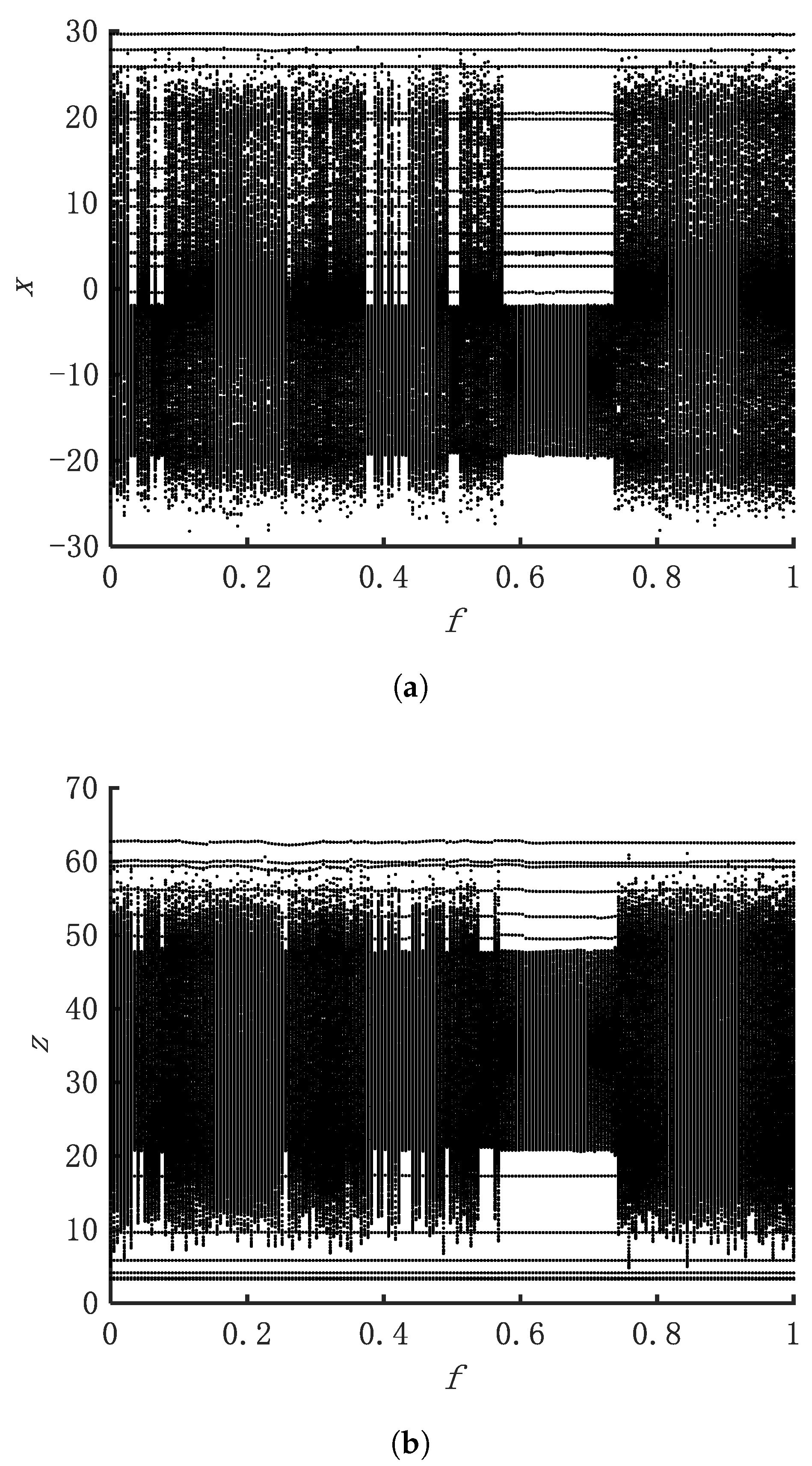
The Yang system follows some general rules of chaotic systems for weak harmonic detection. Increasing the system’s chaotic capacity can improve the system’s resistance to random noise and periodic noise, but it will reduce the detection accuracy of weak harmonic signals. The chaotic capacity is also the degree of confusion in the bifurcation diagram of the system. Since both the Yang and Chen systems can be considered as evolving from the Lorenz system, this conclusion is applicable to all dissipative “Lorenz-like systems”. According to engineering noise environments and engineering precision requirements, the system chaos capacity is modified by modifying the system equations to obtain the best system suitable for the current noise environment so as to obtain the best comprehensive detection performance.

(5)

Compared with non-dissipative chaotic systems such as Duffing systems, dissipative chaotic systems have a higher detection accuracy and anti-noise performance, but the detection efficiency is slightly reduced. Dissipative chaotic systems are more suitable for extremely noisy environments and engineering scenarios that require a high detection accuracy, while non-dissipative chaotic systems are more suitable for engineering scenarios that generally require precision and real-time detection performance.

References

1. Maria, F.; Dimitrios, R.; Stefanos, P. Decision Support System for Emergencies in Microgrids. Sensors 2022, 22, 9457. [Google Scholar]
2. Miao, M.; Yong, L.; Wang, Z.; Ou, L.; Fang, L.; Kwang, L.; Yi, T. An Emergency Energy Management for AC/DC Micro-grids in Industrial Park. IFAC-PapersOnLine 2018, 51, 251–255. [Google Scholar] [CrossRef]
3. Xu, Y.; Du, Y.; Li, Z.; Xi, L.; Liu, Y. Harmonic Parameter Online Estimation in Power System Based on Hann Self-Convolving Window and Equidistant Two-Point Interpolated DFT. MAPAN 2019, 35, 69–79. [Google Scholar] [CrossRef]
4. Chen, L.; Chen, G. Harmonic Detection and Control of Power System Based on Improved EEMD Algorithm. In Proceedings of the 2015 3rd International Conference on Advances in Energy and Environmental Science, Zhuhai, China, 25–26 July 2015. [Google Scholar]
5. Wei, W.; Liu, Z.; Lin, C.; Sha, W. Harmonic Detection of Power System Based on SVD and EMD. In Proceedings of the 2013 Ninth International Conference on Computational Intelligence and Security, Emei Mountain, China, 14–15 December 2013; pp. 185–189. [Google Scholar]
6. Qi, D.; Wang, W.; Quan, G.; Long, Q.; Jin, Y. Power system harmonic detection based on second-order synchrosqueezing wavelet transform. Int. J. Power Energy Syst. 2018, 38, 144–151. [Google Scholar] [CrossRef]
7. Fan, C.; Chen, D.; Fan, L. Research of two phase flow signal denoising based on fractional wavelet transform. In Proceedings of the 2018 IEEE 7th Data Driven Control and Learning Systems Conference (DDCLS), Enshi, China, 25–27 May 2018; pp. 698–703. [Google Scholar]
8. Nan, W.; Zhao, H. A Variable Step Size LMS Adaptive Filtering Algorithm Based on Maximum Correntropy Criterion for Identification of Low Frequency Oscillation Modes. IFAC-PapersOnLine 2019, 52, 163–167. [Google Scholar] [CrossRef]
9. Raman, L.K.; Gopal, Y.; Birla, D.; Lalwani, M. Effect of fault classification and detection in transmission line using wavelet detail coefficient. Int. J. Comput. Aided Eng. Technol. 2022, 17, 288. [Google Scholar] [CrossRef]
10. Benzi1, R.; Sutera, A.; Vulpiani, A. The mechanism of stochastic resonance. J. Phys. A Math. Gen. 1981, 14, L453. [Google Scholar] [CrossRef]
11. Gammaitoni, L.; Marchesoni, F.; Menichella-Saetta, E.; Santucci, S. Stochastic Resonance in Bistable Systems. Phys. Rev. Lett. 1989, 62, 349–352. [Google Scholar] [CrossRef]
12. Gang, H.; Nicolis, G.; Nicolis, C. Periodically forced Fokker–Planck equation and stochastic resonance. Phys. Rev. A 1990, 42, 2030–2041. [Google Scholar] [CrossRef]
13. Huang, D.; Yang, J.; Zhang, J.; Liu, H. An improved adaptive stochastic resonance with general scale transformation to extract high-frequency characteristics in strong noise. Int. J. Mod. Phys. B 2018, 32, 1850185. [Google Scholar] [CrossRef]
14. Zhang, Y.; Zhang, Y.; Wu, J. SSR detection method based on normalized adaptive stochastic resonance. In Environmental Science and Information Application Technology; CRC Press: Boca Raton, FL, USA, 2015. [Google Scholar]
15. Han, D.; Su, X.; Shi, P. Weak Fault Signal Detection of Rotating Machinery Based on Multistable Stochastic Resonance and VMD-AMD. Shock Vib. 2018, 2018, 4252438. [Google Scholar] [CrossRef]
16. Hong-Yan, X.; Wei, X. The neural networks method for detecting weak signals under chaotic background. Acta Phys. Sin. 2007, 56, 3771–3776. [Google Scholar] [CrossRef]
17. Kumar, P.; Narayanan, S.; Gupta, S. Bifurcation analysis of a stochastically excited vibro-impact Duffing-Van der Pol oscillator with bilateral rigid barriers. Int. J. Mech. Sci. 2017, 127, 103–117. [Google Scholar] [CrossRef]
18. Hou, J.; Yan, X.P.; Li, P.; Hao, X.H. Weak wide-band signal detection method based on small-scale periodic state of Duffing oscillator. Chin. Phys. B 2018, 27, 030702. [Google Scholar] [CrossRef]
19. Liu, X.C.; Li, P.P. Weak Signal Detection Based on the Nonlinear Dynamic Model. Appl. Mech. Mater. 2012, 157, 887–891. [Google Scholar] [CrossRef]
20. Zhao, H.; Lin, Y.; Dai, Y. Hidden Attractors and Dynamics of a General Autonomous van der Pol-Duffing Oscillator. Int. J. Bifurc. Chaos 2014, 24, 1450080. [Google Scholar] [CrossRef]
21. Wang, Q.; Yang, Y.; Zhang, X. Weak signal detection based on Mathieu-Duffing oscillator with time-delay feedback and multiplicative noise. Chaos Solitons Fractals 2020, 137, 109832. [Google Scholar] [CrossRef]
22. Hu, N.; Wen, X. The application of Duffing oscillator in characteristic signal detection of early fault. J. Sound Vib. 2003, 268, 917–931. [Google Scholar] [CrossRef]
23. Zhao, Z.; Yang, S. Application of van der Pol–Duffing oscillator in weak signal detection. Comput. Electr. Eng. 2015, 41, 1–8. [Google Scholar]
24. Yang, Q.; Dong, K.; Song, J.; Jin, F.; Mo, W.; Hui, Y. A Weak Signal Detection Method Based on Memristor-Based Duffing-Van der pol Chaotic Synchronization System. In Proceedings of the 13th International Conference on Communication Software and Networks (ICCSN), Chongqing, China, 4–7 June 2021. [Google Scholar]
25. Xiao, F.; Yan, G.; Zhang, X. Effect of signal modulating noise in bistable stochastic dynamical systems. Chin. Phys. 2003, 12, 946. [Google Scholar]
26. Peter, J.; Peter, H. Amplification of small signals via stochastic resonance. Phys. Rev. A 1991, 44, 8032–8042. [Google Scholar]
27. Yong, L.; Tai, W.; Yan, G.; Zhen, W. Study of the property of the parameters of bistable stochastic resonance. Acta Phys. Sin. 2007, 56, 30. [Google Scholar]
28. Li, H.; Bao, R.; Xu, B.; Zheng, J. Intrawell stochastic resonance of bistable system. J. Sound Vib. 2004, 272, 155–167. [Google Scholar] [CrossRef]
29. Yim, M.Y.; Liu, K.L. Linear response and stochastic resonance of subdiffusive bistable fractional Fokker–Planck systems. Phys. A Stat. Mech. Its Appl. 2006, 369, 329–342. [Google Scholar] [CrossRef]
30. Guo, L.; Guang, W.; Jin, W.; Xue, W. A Novel Underwater Location Beacon Signal Detection Method Based on Mixing and Normalizing Stochastic Resonance. Sensors 2020, 50, 1292. [Google Scholar]
31. Leng, Y.; Wang, T. Numerical research of twice sampling stochastic resonance for the detection of a weak signal submerged in a heavy noise. Acta Phys. Sin. 2003, 52, 2432–2437. [Google Scholar] [CrossRef]
32. Wang, M.J.; Zeng, Y.C.; Chen, G.H.; He, J. Nonresonant parametric control of Chen’s system. Acta Phys. Sin. 2011, 60, 10509. [Google Scholar] [CrossRef]
33. Yue, L.; Bao, Y.; Yao, S. Chaos-based weak sinusoidal signal detection approach under colored noise background. Acta Phys. Sin. 2003, 52, 526. [Google Scholar] [CrossRef]
Figure 1. Potential function curve of a bistable system.
Electronics 12 03896 g001
Figure 2. Schematic diagram of a stochastic resonance proton model.
Electronics 12 03896 g002
Figure 3. A model of a stochastic resonance frequency detection system.
Electronics 12 03896 g003
Figure 4. Cascade stochastic resonance frequency detection system model.
Electronics 12 03896 g004
Figure 5. Yang system state variable bifurcation diagram. (a) x f ; (b) z f .
Electronics 12 03896 g005
Figure 6. Phase trajectories and attractor distribution diagrams of critical Yang systems.
Electronics 12 03896 g006
Figure 7. Phase trajectories and attractor distribution of the Yang system (f = 0.5705277) s.
Electronics 12 03896 g007
Figure 8. Chen system state variable bifurcation diagram. (a) x f ; (b) z f .
Electronics 12 03896 g008aElectronics 12 03896 g008b
Figure 9. Phase trajectories and attractor distribution diagrams of critical Chen systems.
Electronics 12 03896 g009
Figure 10. Phase trajectories and attractor distribution of the Chen system (f = 0.7014001825).
Electronics 12 03896 g010
Figure 11. Single-well random resonance harmonic detection results. (a) −20 dB original signal waveform; (b) −20 dB original signal spectrum; (c) −20 dB single-well stochastic resonance output signal waveform; (d) −20 dB single-trap stochastic resonance output signal spectrum; (e) −20 dB two-stage cascaded single-trap stochastic resonance output signal waveform; (f) −20 dB two-stage cascaded single-trap stochastic resonance output signal spectrum; (g) −30 dB original signal waveform; (h) −30 dB original signal spectrum; (i) −30 dB single-trap stochastic resonance output signal waveform; (j) −30 dB single-trap stochastic resonance output signal spectrum; (k) −30 dB two-stage cascaded single-trap stochastic resonance output signal waveform; (l) −30 dB two-stage cascaded single-hole random resonant output signal spectrum.
Electronics 12 03896 g011aElectronics 12 03896 g011bElectronics 12 03896 g011c
Figure 12. Experimental results of DC transmission line voltage fluctuation detection. (a) Original input signal; (b) Bistable system stochastic resonance output signal; (c) Stochastic resonance follows the system output signal; (d) Stochastic resonance output signal of the two-stage cascaded bistable system; (e) Two-level cascaded stochastic resonance follows the output signal of the system.
Electronics 12 03896 g012aElectronics 12 03896 g012b
Figure 13. Experimental results of generator speed fluctuation detection. (a) Original input signal; (b) bistable system stochastic resonance output signal; (c) stochastic resonance follows the system output signal; (d) stochastic resonance output signal of the two-stage cascaded bistable system; (e) two-level cascaded stochastic resonance follows the output signal of the system.
Electronics 12 03896 g013
Figure 14. Experimental results of low-frequency oscillation signal detection. (a) Noise-free low-frequency oscillation signal; (b) low-frequency oscillation signal in a −20 dB noise environment; (c) single-stage bistable system output signal in a −20 dB noise environment; (d) single-stage following system output signal in a −20 dB noise environment; (e) output signal of the secondary following system in a −20 dB noise environment; (f) low-frequency oscillation signal in a −30 dB noise environment; (g) single-stage bistable system output signal in a −30 dB noise environment; (h) single-stage following system output signal in a −30 dB noise environment; (i) output signal of secondary following system in a −30 dB noise environment.
Electronics 12 03896 g014aElectronics 12 03896 g014bElectronics 12 03896 g014c