Genetic Fuzzy Inference System-Based Three-Dimensional Resolution Algorithm for Collision Avoidance of Fixed-Wing UAVs

Abstract

Fixed-wing Unmanned Aerial Vehicles (UAVs) cannot fly at speeds lower than critical stall speeds. As a result, hovering during a potential collision scenario, like with rotary-wing UAVs, is impossible. Moreover, hovering is not an optimal solution for Collision Avoidance (CA), as it increases mission time and is innately fuel-inefficient. This work proposes a decentralized Fuzzy Inference System (FIS)-based resolution algorithm that modulates the point-to-point mission path while ensuring the continuous motion of UAVs during CA. A simplified kinematic guidance model with coordinated turn conditions is considered to control the UAVs. The model employs a proportional-derivative control of commanded airspeed, bank angle, and flight path angle. The commands are derived from the desired path, characterized by airspeed, heading, and altitude. The desired path is, in turn, obtained using look-ahead points generated for the target point. The FIS aims to mimic human behavior during collision scenarios, generating modulation parameters for the desired path to achieve CA. Notably, it is also scalable, which makes it easy to adjust the algorithm parameters, as per the required missions, and factors specific to a given UAV. A genetic algorithm was used to optimize FIS parameters so that the distance traveled during the mission was minimized despite path modulation. The proposed algorithm was optimized using a pairwise conflict scenario. The effectiveness of the algorithm was evaluated through a Monte Carlo simulation of random conflict scenarios involving multiple UAVs operating in a confined space.

1. Introduction

Global air traffic is expected to grow annually at a rate of 4.1% [1], and global advanced air mobility of automated aircraft at lower altitudes is expected to grow at a compounded annual growth rate of 22.45% [2]. Unmanned Aerial Vehicles (UAVs) would be an integral part of this future air traffic, used for surveillance, military, transportation, cargo, and many more applications. Thus, given the inevitability of potential collisions among aircraft, Collision Avoidance (CA) algorithms are vital for all UAVs, including fixed-wing UAVs. Fixed-wing UAVs carry many advantages over rotary-wing UAVs like greater speed and endurance, higher payload capacity for the same endurance, lower maintenance, lower noise levels, etc., which could be essential for many emergency, reconnaissance, and cargo missions. However, the formulation of CA algorithms is challenging for fixed-wing UAVs. Unlike rotary-wing UAVs, fixed-wing UAVs cannot hover, or even slow down below critical stall speeds during potential collision scenarios. Hovering is also a non-optimal solution for CA as it increases mission time and is innately fuel-inefficient. Thus, this work proposes a decentralized Fuzzy Inference System (FIS)-based resolution algorithm that modulates the point-to-point mission path while ensuring the continuous motion of UAVs during CA. This algorithm, ensuring continuous motion, could likewise provide an efficient solution for CA in rotary-wing UAVs, eliminating the need for hover-based solutions in numerous potential collision scenarios.

Aircraft CA System (ACAS) II is the most common method of CA in crewed aircraft. It is implemented as Traffic CAS (TCAS) II, which provides traffic advisory for warning and resolution advisory for appropriate CA maneuvers to the pilots [3]. However, TCAS II has several limitations, encompassing the provision of resolutions exclusively within the vertical plane like climb, descent, or level flight, and these resolutions are designed for specific encounter geometries; furthermore, TCAS II operates deterministically [4]. The review and analysis of TCAS in [5] also state that expanding the horizontal resolution algorithm will offer superior collision detection and resolution performance. Similarly, the newly proposed method of ACAS X and its variation ACAS Xu for unmanned aircraft encourage the design of resolutions in both vertical and horizontal directions using probabilistic models [6,7]. Therefore, this study proposes to generate resolutions in both vertical and horizontal directions.

A vast number of research studies and algorithms have been proposed for the CA of aircraft, widely classified by Kuchar et al. [8] as prescribed, optimized, force field, or manual. With the advancement of navigation and control technologies for UAVs, CA algorithms can be further classified into various domains, including path planning, conflict resolution, potential function, geometric guidance, and motion planning [9,10]. However, it is essential to note that many of these approaches primarily cater to rotary-wing UAVs capable of stopping and hovering, rendering them less suitable for fixed-wing UAVs. For fixed-wing aircraft, a range of geometric approaches, such as forming circular arcs or Three-Dimensional (3D) trajectories [11,12,13], velocity modulation in the horizontal plane [14], velocity obstacle concepts [15,16,17,18], differential geometry concepts [19], and the use of collision cones [20,21], have been proposed. While these methods provide some applicability to fixed-wing aircraft, they may suffer from limitations such as high computational demands and a lack of intuitive understanding. Furthermore, some concepts involve potential/force fields modified or reformulated with UAV’s physical constraints for better real-life performance [22,23,24], or enhanced and optimized using evolutionary methods to avoid local minima problems [22,25,26]. Unfortunately, many force field methods, like the optimized path planning-based approach of the 3D vector field histogram [27] are predominantly suited for rotary-wing UAVs and may not translate well to fixed-wing UAV scenarios. While path planning-based methods offer high accuracy, some of them, like combining differential game problems with tree-based path planning [28], utilizing reinforcement learning for UAV guidance [29], optimizing flight trajectory with a bank-turn mechanism [30], employing the Radau-pseudospectral approach [31], applying probabilistic methods in collision detection [32], or generating an automated distributed policy for multi-robot motion planning [33], may face significant computational challenges when implemented in real time for small UAVs. Analytical formulations such as the speed approach [34] and the use of buffered Voronoi Cells for path planning [35], though computationally efficient, may lack intuitive understanding and require specialized expertise to implement effectively.

Humans, on the other hand, are innately capable of avoiding collision intuitively [36,37]. So, in recent times, fuzzy logic that emulates the human way of decision making with the linguistic characterization of numerical variables has been gaining popularity in devising CA algorithms in UAVs. This research also uses an FIS to avoid computational complexity while also providing an intuitive understanding of the approach. Just like pilots who perform CA maneuvers manually based on their visual perception and flight instrument information about incoming static or dynamic obstacles, the proposed algorithm also takes into account the sensor readings for incoming intruders to modulate the current path and avoid collisions. Previously, fuzzy logic for CA was predominantly researched in surface vehicles [38,39,40,41]. Now, research on the use of fuzzy logic for CA in UAVs is also gaining traction. For instance, a fuzzy-based aircraft CA system capable of generating an alert of a potential midair collision while taking control if no preventive action is taken within a specified time was proposed by Younas et al. [42]. Choi et al. [43] used an FIS to improve the performance of their enhanced potential field-based CA. Likewise, several basic avoidance methods have been devised to avoid collision using fuzzy logics [44,45,46]. However, most of them are suitable for rotary-wing UAVs. Cook et al. [47] used a fuzzy logic-based approach to help mitigate the risk of collisions among aircraft, including fixed-wing and quadcopter, using separation assurance and CA techniques.

Although similar to the CA logic of [47], which directly generates low-level control input like turn rate using intuitively defined FISs, this work proposes a 3D Collision Avoidance Fuzzy Inference System (3D-CAFIS) to modulate the path variables—heading, velocity, and altitude of the UAVs. Thus, the UAV performs both horizontal and vertical maneuvers. The modulation is based on the relative states of the UAV in consideration, the own-ship, with respect to the nearest intruder or obstacle point. Moreover, a Genetic Algorithm (GA) was used to optimize the FISs such that the distance traveled during the mission is minimal despite path modulation while ensuring separation during CA is above the appropriate threshold. FIS optimization was conducted using a training scenario of three basic pairwise conflicts. The algorithm’s validity can be confirmed using formal methods, which will be similar to that outlined in [47], as the basic approach of defining the FISs for this study was similar. However, due to the complexity of the algorithm with many variables, the effectiveness of the algorithm is evaluated through multiple simulations of randomly generated UAV missions within a closed functional space.

The paper begins by introducing the system architecture and the UAV model utilized in this study in Section 2. Next, Section 3 provides a step-by-step explanation of the proposed algorithm. Section 4 presents the findings from our simulation studies. Lastly, Section 5 offers a summary of this work and addresses future works.

2. System Modeling

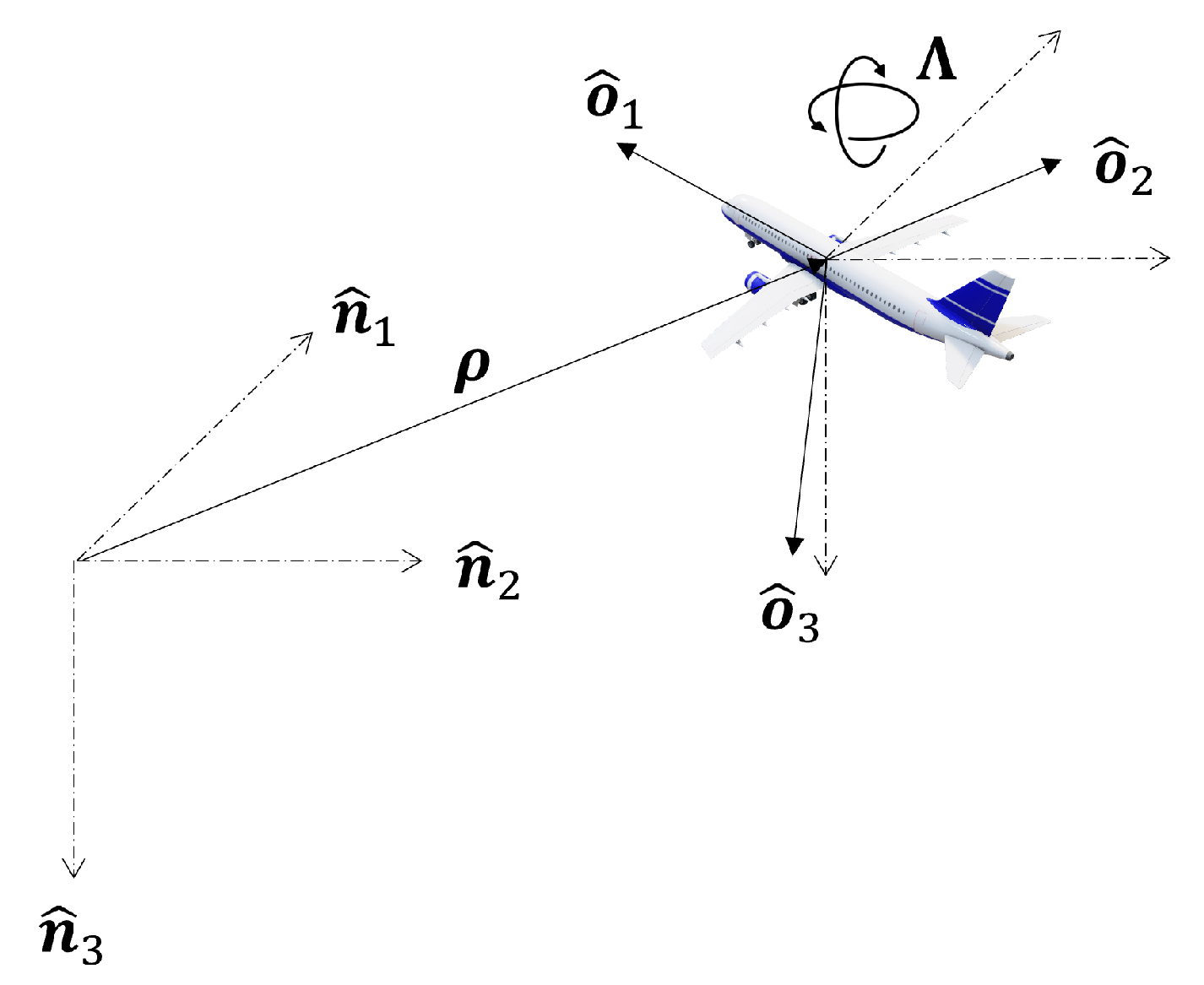
UAVs operate in the N-frame. Hereafter, ‘own-ship’ refers to the UAV currently executing the CA algorithm, while ‘intruders’ denote other UAVs in the airspace. The own-ship’s body frame is designated as the O-frame and the intruder’s as the I-frame. A UAV’s position in the N-frame is defined by ${}^N\mathit{\rho }$, and its attitude is represented by the 3-2-1 set of Euler angles ($\mathbf{\Lambda }={\left[\psi ,\theta ,\varphi \right]}^{\top }$), as shown in Figure 1. For simplicity, one omits the N-frame expression.

Furthermore, the state of a fixed-wing UAV can be comprehensively defined with parameters including airspeed (${\mathit{\nu }}_{\mathrm{air}}$), ground speed (${\mathit{\nu }}_{\mathrm{ground}}$), wind velocity (${\mathit{\nu }}_{\mathrm{wind}}$), $\alpha$, $\beta$, $\chi$, and $\gamma$, as shown in Figure 2.

The UAV’s attitude can also be represented in the G-frame, obtained using the 3-2-1 set of Euler angles (${}^G\mathbf{\Lambda }={\left[\chi ,\gamma ,\varphi \right]}^{\top }$). Consequently, the UAV state space vector considered is $\mathbf{p}={\left[{\mathit{\rho }}^{\top },{\nu }_{\mathrm{air}},{}^G\mathbf{\Lambda },{\dot{\varphi }}^{\top }\right]}^{\top }$. Note that ${\nu }_{\mathrm{air}}$ is the norm of ${\mathit{\nu }}_{\mathrm{air}}$.

A basic system architecture for the waypoint control and CA of a UAV is depicted in Figure 3.

In summary, the significance of each block is explained below:

• Waypoint Follower (Section 3.1) determines the desired path along with the desired change variables based on set waypoints.
• Collision Detection (CD) (Section 3.2) checks whether the own-ship is on a collision course with an intruder using range-bearing sensors and modified TCAS logic.
• 3D-CAFIS (Section 3.3) generates modulation parameters based on relative states obtained from CD using the proposed FIS tree. These parameters modulate the desired path obtained from the waypoint follower, thus avoiding potential collisions.
• Controller (Section 3.4) calculates control commands based on the path, either from the waypoint follower or, if CA is initiated, from the 3D-CAFIS, to control the UAV.
• UAV Plant represents the kinematic mathematical model of a fixed-wing UAV that simulates UAV motion.
• Sensors consist of a global positioning system and an inertial measurement unit for determining the position, velocity, and angular velocity of the own-ship, along with a range-bearing sensor that measures the relative position of intruders in airspace.
• State Estimator utilizes filtering techniques to estimate the position and attitude of the UAV. This is not within the scope of this research.

Here, UAVs are controlled via a proportional-derivative control of ${\nu }_{\mathrm{air}}$, $\gamma$, and $\varphi$. The subsequent kinematic guidance model for the UAV is given by [48]

$$\begin{array}{cc}\hfill \dot{\mathit{\rho }}& =C_{N/G}{}^G{\mathit{\nu }}_{\mathrm{ground}},\hfill \end{array}$$

(1)

$$\begin{array}{cc}\hfill {\dot{\nu }}_{\mathrm{air}}& =k_{{\nu }_{\mathrm{air}}}\left({\nu }_{\mathrm{air}}^{\mathrm{c}}-{\nu }_{\mathrm{air}}\right),\hfill \end{array}$$

(2)

$$\begin{array}{cc}\hfill \dot{\gamma }& =k_{\gamma }\left({\gamma }^{\mathrm{c}}-\gamma \right),\hfill \end{array}$$

(3)

$$\begin{array}{cc}\hfill \dot{\chi }& =\frac{gcos(\chi -\psi )}{{\nu }_{\mathrm{ground}}}tan\varphi ,\hfill \end{array}$$

(4)

$$\begin{array}{cc}\hfill \ddot{\varphi }& =k_{\varphi }\left({\varphi }^{\mathrm{c}}-\varphi \right)+k_{\dot{\varphi }}\left(-\dot{\varphi }\right),\hfill \end{array}$$

(5)

where ${}^G{\mathit{\nu }}_{\mathrm{ground}}={\left[{\nu }_{\mathrm{ground}},0,0\right]}^{\top }$ is the ground speed vector in the G-frame, while $k_{\gamma }$, $k_{{\nu }_{\mathrm{air}}}$, $k_{\varphi }$, and $k_{\dot{\varphi }}$ are gain values tuned to achieve smoother flight maneuvers. Note that under wind-less conditions, ${\nu }_{\mathrm{air}}={\nu }_{\mathrm{ground}}$, $\psi =\chi$, and $\theta =\gamma$. For simplicity, UAVs are assumed to be in a coordinated-turn condition with zero side-slip and zero angles of attack. The relationship between the course angle and bank angle is expressed in Equation (4). Also, ${\varphi }^{\mathrm{c}}$, ${\gamma }^{\mathrm{c}}$, and ${\nu }_{\mathrm{air}}^{\mathrm{c}}$ serve as the command variables for controlling the UAV.

3. Proposed Method

3.1. Waypoint Follower

The waypoint follower is a path generator that calculates the desired variables, fully defining a trajectory for the UAV during a mission to a waypoint. This approach draws inspiration from pure pursuit control [28], incorporating the look-ahead point position vector (${\mathit{\rho }}^l$) and l into the calculation of the desired variables. Given a waypoint position vector (${\mathit{\rho }}^{\mathrm{w}}$) in the N-frame, its relative position vector with respect to the own-ship is expressed as follows:

$${\mathit{\rho }}_{\mathrm{w}/O}={\mathit{\rho }}^{\mathrm{w}}-{\mathit{\rho }}_O.$$

(6)

Then, the look-ahead point position vector is obtained via

$${\mathit{\rho }}^l=\mathit{\rho }+l{\widehat{\mathit{\rho }}}_{\mathrm{w}/O},$$

(7)

and the desired path requisites are calculated as follows:

$$\begin{array}{cc}\hfill {\chi }^{\mathrm{d}}& ={tan}^{-1}\left(\frac{{\rho }_2^l-{\rho }_2}{{\rho }_1^l-{\rho }_1}\right),\hfill \end{array}$$

(8)

$$\begin{array}{cc}\hfill \Delta {\chi }^{\mathrm{d}}& ={\chi }^{\mathrm{d}}-\chi ,\hfill \end{array}$$

(9)

$$\begin{array}{cc}\hfill h^{\mathrm{d}}& =-{\rho }_3^l,\hfill \end{array}$$

(10)

$$\begin{array}{cc}\hfill \Delta h^{\mathrm{d}}& =h^{\mathrm{d}}-h.\hfill \end{array}$$

(11)

The desired airspeed (${\nu }_{\mathrm{air}}^{\mathrm{d}}$) is determined based on the mission requirements. In this research, it is assumed to be equal to an optimal airspeed (${\nu }_{\mathrm{air}}^{\mathrm{opt}}$), which gradually decreases quadratically as the target point is approached. Thus, the desired path is characterized by ${\nu }_{\mathrm{air}}^{\mathrm{d}}$, ${\chi }^{\mathrm{d}}$, $\Delta {\chi }^{\mathrm{d}}$, $h^{\mathrm{d}}$, and $\Delta h^{\mathrm{d}}$.

3.2. Collision Detection (CD)

The CD begins with intruder detection, where the intruder’s presence is initially identified using the intruder’s 3D spherical coordinates (${\left[r,\eta ,ϵ\right]}^{\top }$) acquired from the onboard range-bearing sensor. These coordinates are then transformed into Cartesian form to establish the separation between the own-ship and the intruder (${}^O\mathbf{s}={}^O{\mathit{\rho }}_{I/O}$). The horizontal and vertical views of two potentially colliding UAVs—one own-ship in the O-frame and another intruder in the I-frame—are depicted in Figure 4. Figure 4a shows the top-down view of the two UAVs, while Figure 4b offers a side view of the UAVs on a vertical plane. Here, ${\mathit{\nu }}_O$ and ${\mathit{\nu }}_I$ are the velocities of the own-ship and intruder, respectively, and their relative velocity is expressed as ${\mathit{\nu }}_{O/I}$. Also, ${\psi }_M$ is the angle formed by $\mathbf{s}$ with respect to ${\widehat{\mathit{n}}}_1$, while ${\chi }_{O/I}$ is the relative course angle of the own-ship with respect to the intruder.

The relative velocity and separation between the own-ship and the intruder play a crucial role in CD. These values are essential for applying the CD logic provided by TCAS II, which assesses whether the own-ship is on a potential collision course with an intruder. To begin, the relative velocity of the intruder with respect to the own-ship, as observed in the N-frame, can be determined using the transport theorem, and this is expressed in the O-frame as follows:

$${}_N^O\dot{\mathbf{s}}={}_O^O\dot{\mathbf{s}}+{}^O{\mathit{\omega }}_{O/N}\times {}^O\mathbf{s}.$$

(12)

Here, ${}_O^O\dot{\mathbf{s}}$ is determined with successive range-bearing measurements as follows:

$${}_O^O\dot{\mathbf{s}}=\frac{{\left({}^O\mathbf{s}\right)}_t-{\left({}^O\mathbf{s}\right)}_{t-\Delta t}}{\Delta t},$$

(13)

where $\Delta t$ is the time interval between two successive measurements. Also, the angular velocity in the O-frame is derived from the inertial measurement unit.

Now, one introduces an M-frame achieved by rotating the N-frame about ${\widehat{\mathit{n}}}_3$ by ${\psi }_M$. The horizontal and vertical separations (x and z) and their respective closure rates (${\nu }_x$ and ${\nu }_z$) can be determined from the relative separation and relative velocity when expressed in the M-frame, respectively, as shown below:

$$\begin{array}{cc}\hfill {}^M\mathbf{s}& =C_{M/N}{C}_{N/O}{}^O\mathbf{s}={\left[x,y,z\right]}^{\top },\hfill \end{array}$$

(14)

$$\begin{array}{cc}\hfill {}_N^M{\mathit{\nu }}_{O/I}& =-C_{M/N}{C}_{N/O}{}_N^O\dot{\mathbf{s}}={\left[{\nu }_x,{\nu }_y,{\nu }_z\right]}^{\top }.\hfill \end{array}$$

(15)

Note that $z=-h$, and thus, $z^d=-h^d$ and $\Delta z^{\mathrm{d}}=-\Delta h^{\mathrm{d}}$.

The CD is confirmed if the time to the Closest Point of Approach (CPA) is less than the CPA thresholds (${\tau }_{\mathrm{th}}$) in both the horizontal range (${\tau }_x$) and vertical range (${\tau }_z$) directions. These calculations are carried out as described below [49]:

$$\begin{array}{cc}\hfill {\tau }_x& =\left|{\nu }_x\right|/x,\hfill \end{array}$$

(16)

$$\begin{array}{cc}\hfill {\tau }_z& ={\nu }_z/z.\hfill \end{array}$$

(17)

The thresholds are selected using TCAS II logic, which considers the altitude of operation and the sensitivity level [3]. However, since TCAS is designed for large aircraft, and this study focuses on small UAVs, the thresholds are determined based on the specific UAV and sensor limitations. Similarly, ${\chi }_{O/I}$ and ${\psi }_M$ are crucial relative variables for CA. They assist in determining inputs, namely $\Delta {\psi }_M$ and $sign\left(\Delta {\chi }_{O/I}\right)$, for the 3D-CAFIS. In this context, $\Delta {\psi }_M$ indicates the anticipated position of the own-ship with respect to the intruder at the CPA, while $sign\left(\Delta {\chi }_{O/I}\right)$ denotes the direction of relative motion in comparison to the current course angle, thereby distinguishing between collisions in the same direction and opposite directions. These values are calculated as follows:

$$\begin{array}{cc}\hfill \Delta {\psi }_M& ={\chi }_{O/I}-{\psi }_M,\hfill \end{array}$$

(18)

$$\begin{array}{cc}\hfill sign(\Delta {\chi }_{O/I})& =sign({\chi }_{O/I}-{\chi }_O).\hfill \end{array}$$

(19)

However, in cases of slower closure rates, this method could trigger CD alerts even when a significant separation exists. Therefore, when dealing with slower closure rates, a comparison is made between the horizontal and vertical separations against the distance modification threshold (DMOD) and altitude threshold (ZTHR) for the small UAVs, respectively. A collision is assumed if either the horizontal separation is below the threshold ($x_{\mathrm{th}}$) or the vertical separation is below the threshold ($z_{\mathrm{th}}$).

3.3. Three-Dimensional Collision Avoidance Fuzzy Inference System (3D-CAFIS)

3.3.1. Fuzzy Tree

A fuzzy tree is designed to obtain path modulation parameters from the relative variables determined in CD, as shown in Figure 5. The blocks FIS_H1 and FIS_H2 represent FISs that yield modulation parameters $\Delta {\chi }^{\mathrm{ca}}$ and $\Delta {\nu }_x^{\mathrm{ca}}$, respectively, for horizontal maneuvers. Similarly, the blocks FIS_V1 and FIS_V2 are FISs that yield modulation parameters $\Delta h^{\mathrm{ca}}$ and $\Delta {\nu }_z^{\mathrm{ca}}$, respectively, for vertical maneuvers. Ultimately, the outputs $\Delta {\chi }^{\mathrm{ca}}$ and $\Delta h^{\mathrm{ca}}$ serve as inputs to the FIS_W block, yielding ${{\rm Y}}_x$ and ${{\rm Y}}_z$ which are weights for horizontal and vertical maneuvers, respectively. Note that there is an input to the fuzzy tree, $\Delta z^{{\mathrm{d}}^{*}}$, which is a modified version of $\Delta z^{\mathrm{d}}$ designed to induce complementary altitude adjustments between potentially colliding UAVs coming from opposite directions. Its calculation is as follows:

$$\Delta z^{{\mathrm{d}}^{*}}=sign(\Delta {\chi }_{O/I})\Delta z^{\mathrm{d}}$$

(20)

The inputs of each FIS block are normalized using a factor determined according to the potential range of the actual input values, which takes into account factors such as sensor limits, UAV performance limits, and so on. The outputs of the fuzzy tree are derived by multiplying the normalized outputs of the FISs by their respective normalization factors. These factors are determined based on the expected range that the respective outputs can span over the sampling time. The relative variables utilized as inputs for the FIS tree, as well as the modulation parameters for outputs, are presented in

Table 1. FIS tree input and output variables.

Variables	Type	Normalization Factor	Significance
x	Input	$0.4$ nm	Horizontal proximity
z	Input	1562 ft	Vertical proximity
$\Delta {\chi }^{\mathrm{d}}$	Input	$\pi$	Desired course
$\Delta {\psi }_M$	Input	$\pi$	Course direction with respect to intruder
$\left|{\nu }_x\right|$	Input	140 kts	Horizontal closure rate
${\nu }_z$	Input	6000 ft/min	Vertical closure rate
$\Delta z^{{\mathrm{d}}^{*}}$	Input	$42.65$ ft	Desired altitude
$\Delta {\nu }_x^{\mathrm{ca}}$	Output	$1.738$ kts	Horizontal speed modulation
$\Delta {\nu }_z^{\mathrm{ca}}$	Output	$124.45$ ft/min	Vertical speed modulation
$\Delta {\chi }^{\mathrm{ca}}$	Output	65 deg	Course modulation
$\Delta h^{\mathrm{ca}}$	Output	8 ft	Altitude modulation
${{\rm Y}}_x$	Output	1	Intensity of the horizontal maneuvers
${{\rm Y}}_z$	Output	1	Intensity of the vertical maneuvers

, along with their corresponding normalization factor and significance.

For this study, each of the normalized inputs and outputs of the FISs is fuzzified into three Membership Functions (MFs)—two trapezoidal ones at each end and one triangular MF in the middle, as shown in Figure 6. The decision to use three MFs serves a dual purpose. Firstly, it provides simplicity in emulating three fundamental directions or maneuvers associated with human behavior during CA, such as left, center, and right or up, in front, and down. Secondly, the MFs for all inputs and outputs can be symmetrically arranged around the midpoints of their respective ranges, reducing complexity when optimizing using a GA. The specifics of each normalized input and output of the FISs are provided in

Table 2. Normalized variable details.

Variables	Input for	Output of	Range	MFs
				Trapezoid	Triangle	Trapezoid
$\widehat{x}$	FIS_H1, FIS_H2, FIS_V1	None	[0, 1]	Close	Near	Far
$\widehat{z}$	FIS_V1, FIS_V2	None	[$-1$, 1]	Above	In-line	Below
$\Delta {\widehat{\chi }}^{\mathrm{d}}$	FIS_H1	None	[$-1$, 1]	Left	Center	Right
$\Delta {\widehat{\psi }}_M$	FIS_H1	None	[$-1$, 1]	Left	Center	Right
$\left|{\widehat{\nu }}_x\right|$	FIS_H2	None	[0, 1]	Slow	Medium	Fast
${\widehat{\nu }}_z$	FIS_V2	None	[$-1$, 1]	Upward	Straight	Downward
$\Delta {\widehat{z}}^{{\mathrm{d}}^{*}}$	FIS_H1	None	[$-1$, 1]	Above	In-line	Below
$\Delta {\widehat{\nu }}_x^{\mathrm{ca}}$	None	FIS_H1	[$-1$, 1]	Speed-Down	Continue	Speed-Up
$\Delta {\widehat{\nu }}_z^{\mathrm{ca}}$	None	FIS_V1	[$-1$, 1]	Climb	Continue	Descend
$\Delta {\widehat{\chi }}^{\mathrm{ca}}$	FIS_W	FIS_H2	[$-1$, 1]	Go-Left	Continue	Go-Right
$\Delta {\widehat{h}}^{\mathrm{ca}}$	FIS_W	FIS_V2	[$-1$, 1]	Go-Down	Continue	Go-Up
${{\rm Y}}_x$	None	FIS_W	[0, 1]	Low	Medium	High
${{\rm Y}}_z$	None	FIS_W	[0, 1]	Low	Medium	High

.

The rule base is developed based on basic human intuition regarding potential collision scenarios. For instance, in FIS_H1:

• IF $\widehat{x}$ is Close, meaning that the own-ship and the intruder are nearly colliding, AND $\Delta {\widehat{\psi }}_M$ is Left, meaning that the own-ship is positioned to the left of the intruder at CPA, AND $\Delta {\widehat{\chi }}^{\mathrm{d}}$ is Left, meaning that the desired look-ahead point is to the left of the own-ship, THEN $\Delta {\widehat{\chi }}^{\mathrm{ca}}$ is Go-Left, signifying that the own-ship’s path is to be modulated to the left.
• IF $\widehat{x}$ is Far, meaning that the own-ship and the intruder are still considerably apart, AND $\Delta {\widehat{\psi }}_M$ is Center, meaning that the own-ship is nearly colliding head-on with the intruder at CPA, AND $\Delta {\widehat{\chi }}^{\mathrm{d}}$ is Center, meaning that the desired look-ahead point is directly ahead of the own-ship, THEN $\Delta {\widehat{\chi }}^{\mathrm{ca}}$ is Continue, indicating that the own-ship’s path should not be significantly modulated.

Similarly, in FIS_V2:

• IF ${\widehat{\nu }}_z$ indicates an Upward motion, implying that the own-ship is ascending relative to the intruder, AND $\widehat{z}$ denotes Above, meaning that the intruder is positioned higher than the own-ship, THEN $\Delta {\widehat{\nu }}_z^{\mathrm{ca}}$ signifies Descend, meaning that the own-ship’s vertical velocity component should be adjusted to descend.
• IF ${\widehat{\nu }}_z$ is a Downward motion, meaning that the own-ship is descending relative to the intruder, AND $\widehat{z}$ signifies In-line, meaning that the intruder is directly ahead of the own-ship, THEN $\Delta \widehat{\nu }{)}_z^{\mathrm{ca}}$ signifies Climb, implying that the own-ship’s vertical velocity component should be adjusted to climb.

Thus, a total of 81 rules were defined—27 rules for FIS_H1 and FIS_V1 each and 9 rules for FIS_H2, FIS_V2, and FIS_W each.

It is also worth noting that, to simulate a real-life environment where perfectly symmetric conflict scenarios are unlikely, slight randomness is introduced to the relative variables $\Delta {\psi }_M$ and z. Similarly, for special ‘Top-Down’ scenarios in which the intruder is directly above or below the own-ship and both of them are moving in the same direction towards a potential collision, the modulation parameters for vertical maneuvers, $\Delta {\chi }^{\mathrm{ca}}$ and $\Delta h^{\mathrm{ca}}$, are adjusted as follows:

$$\begin{array}{cc}\hfill \Delta {\nu }_z^{\mathrm{ca}}& =T{D}_{\mathrm{factor}}\times \left|\Delta {\nu }_z^{\mathrm{ca}}\right|,\hfill \end{array}$$

(21)

$$\begin{array}{cc}\hfill \Delta h^{\mathrm{ca}}& =T{D}_{\mathrm{factor}}\times \left|\Delta h^{\mathrm{ca}}\right|,\hfill \end{array}$$

(22)

where $T{D}_{\mathrm{factor}}$ is an arbitrary factor that can be tuned for this special ‘Top-Down’ case. An instance of this scenario is illustrated by the pairwise conflict involving UAVs 5 and 6 in Figure 9a.

3.3.2. Desired Path Modulation

The desired path obtained from the waypoint follower is modulated using modulation parameters obtained from 3D-CAFIS. First, ${\chi }^{\mathrm{c}}$ and $h^{\mathrm{c}}$ are calculated as

$$\begin{array}{cc}\hfill {\chi }^{\mathrm{c}}& ={\chi }^{\mathrm{d}}+{{\rm Y}}_x{\Delta \chi }^{\mathrm{ca}},\hfill \end{array}$$

(23)

$$\begin{array}{cc}\hfill h^{\mathrm{c}}& =h^{\mathrm{d}}+{{\rm Y}}_z{\Delta h}^{\mathrm{ca}}.\hfill \end{array}$$

(24)

Now, the modulation of the desired airspeed begins with the determination of the desired velocity in the M-frame as follows:

$${}^M{\left[{\nu }_x^{\mathrm{d}},{\nu }_y^{\mathrm{d}},{\nu }_z^{\mathrm{d}}\right]}^{\top }=C_{M/N}{C}_{N/O}{}^O{\left[{\nu }_{\mathrm{air}}^{\mathrm{d}},0,0\right]}^{\top }.$$

(25)

Then, ${\nu }_x^{\mathrm{d}}$ and ${\nu }_z^{\mathrm{d}}$ are modulated to obtain the following commanded horizontal and vertical closure rates:

$$\begin{array}{cc}\hfill {\nu }_x^{\mathrm{c}}& ={\nu }_x^{\mathrm{d}}+{{\rm Y}}_x\Delta {\nu }_x^{\mathrm{ca}},\hfill \end{array}$$

(26)

$$\begin{array}{cc}\hfill {\nu }_z^{\mathrm{c}}& ={\nu }_z^{\mathrm{d}}+{{\rm Y}}_z\Delta {\nu }_z^{\mathrm{ca}}.\hfill \end{array}$$

(27)

To avoid extreme deviation from the desired path, one sets ${\nu }_y^{\mathrm{c}}={\nu }_y^{\mathrm{d}}$. The commanded airspeed (${\nu }_{\mathrm{air}}^{\mathrm{c}}$) is obtained from the norm of modulated velocity given below:

$${\mathit{\nu }}_{\mathrm{air}}^{\mathrm{c}}={\left(C_M^N\right)}^{\top }{\left[{\nu }_x^{\mathrm{c}},{\nu }_y^{\mathrm{c}},{\nu }_z^{\mathrm{c}}\right]}^{\top }.$$

(28)

3.4. Controller

The controller block determines the primary control commands: ${\gamma }^{\mathrm{c}}$, ${\varphi }^{\mathrm{c}}$, and ${\nu }_{\mathrm{air}}^{\mathrm{c}}$. It is important to note that when no potential collisions are detected, the values are such that ${\nu }_{\mathrm{air}}^{\mathrm{c}}={\nu }_{\mathrm{air}}^{\mathrm{d}}$, ${\chi }^{\mathrm{c}}={\chi }^{\mathrm{d}}$, and $h^{\mathrm{c}}=h^{\mathrm{d}}$. However, in the presence of a potential collision, ${\gamma }^{\mathrm{c}}$ and ${\varphi }^{\mathrm{c}}$ are determined from the path characterized by ${\nu }_{\mathrm{air}}^{\mathrm{c}}$, ${\chi }^{\mathrm{c}}$, and $h^{\mathrm{c}}$ obtained from the desired path modulation as follows:

$$\begin{array}{cc}\hfill \frac{cos(\chi -\psi )}{{\nu }_{\mathrm{ground}}}tan{\varphi }^{\mathrm{c}}& =k_{\chi }\left({\chi }^{\mathrm{c}}-\chi \right),\hfill \end{array}$$

(29)

$$\begin{array}{cc}\hfill {\nu }_{\mathrm{air}}sin\left({\gamma }^{\mathrm{c}}\right)& =min\left(max\left(k_z\left(h^{\mathrm{c}}-h\right),-{\nu }_{\mathrm{air}}\right),{\nu }_{\mathrm{air}}\right).\hfill \end{array}$$

(30)

Here, $k_h$ and $k_{\chi }$ are gain values tuned to achieve smoother bank and flight path angles. Lastly, ${\gamma }^{\mathrm{c}}$, ${\varphi }^{\mathrm{c}}$, and ${\nu }_{\mathrm{air}}^{\mathrm{c}}$ are the control commands used to control the UAV toward the desired waypoint while avoiding collision. Equation (30) represents a saturation function designed to limit the excessive vertical speed of the UAV. However, before being transmitted to the flight controller, these control commands are subjected to limits set by the physical and aerodynamic limitations of respective UAVs.

The algorithm, presented and discussed in Section 3.1, Section 3.2, Section 3.3 and Section 3.4, is summarized in Figure 7.

3.5. 3D-CAFIS Optimization Using the Genetic Algorithm (GA)

The GA is an evolutionary optimization algorithm that tunes system parameters by maximizing a fitness function (or minimizing a cost function) via the selection, crossover, and mutation of chromosomes comprising those parameters. Figure 8 depicts a fundamental FIS optimization diagram employing a GA. The rule base and the MFs constitute the knowledge base of the FIS. To fully define the proposed fuzzy tree, a total of 224 parameters must be tuned. These parameters include 4 for defining 2 trapezoidal MFs and 3 for defining 1 triangular MF for each of the 13 variables within the fuzzy tree, resulting in a total of 143 parameters, as well as 81 parameters corresponding to each of the rules. The computational effort required for optimizing the proposed FIS is significantly reduced through the utilization of constant rules chosen based on human intuition. Additionally, the symmetry of MFs within each FIS is maintained by considering only two tunable parameters (a and b), as shown in Figure 6. Consequently, the total number of tunable parameters is reduced to 26.

It is important to note that this optimization process is carried out before a specific mission type for a given UAV. Once optimized, the 3D-CAFIS algorithm is seamlessly integrated into the UAV system, enabling real-time CA during potentially conflicting scenarios.

This study involves the formulation of a Cost Function ($CF$) aimed at minimizing collisions, reducing path deviation during CA, and ensuring adequate separation to prevent potential collisions and preemptive collisions. The $CF$ is defined as follows:

$$minCF={\int }_{t=0}^{t_f}{\delta }_1{\sigma }_1\left(t\right)+{\delta }_2{\sigma }_2\left(t\right)+{\delta }_3{\sigma }_3\left(t\right)+{\delta }_4{\sigma }_4\left(t\right),$$

(31)

where $t_f$ is the total simulation time. ${\sigma }_1$, ${\sigma }_2$, ${\sigma }_3$, and ${\sigma }_4$ are the collision cost to prevent a collision, the route cost to minimize the total travel distance, the separation cost to maintain proximity to the given separation threshold ($s_{\mathrm{th}}$), and the time of collision cost to avoid early collisions, respectively. Correspondingly, ${\delta }_i$ serves as the weight assigned to each respective cost, which can be tuned to achieve mission-critical performance objectives. Each of these costs at a given instant t is calculated as follows:

$$\begin{array}{cc}\hfill {\sigma }_1\left(t\right)& =\sum _{i=1}^{n_{\mathrm{coll}}}i,\hfill \end{array}$$

(32)

$$\begin{array}{cc}\hfill {\sigma }_2\left(t\right)& =\sum _{i=1}^{n_{\mathrm{uavs}}}∥{\mathit{\rho }}_{{(\mathrm{w}/O)}_i}∥,\hfill \end{array}$$

(33)

$$\begin{array}{cc}\hfill {\sigma }_3\left(t\right)& =\sum _{i=1}^{n_{\mathrm{uavs}}}{s}_{\mathrm{th}}-∥{\mathbf{s}}_i∥,\hfill \end{array}$$

(34)

$$\begin{array}{cc}\hfill {\sigma }_4\left(t\right)& =\sum _{i=1}^{n_{\mathrm{coll}}}{t}_f-t_{\mathrm{coll},i},\hfill \end{array}$$

(35)

where $n_{\mathrm{uavs}}$ is the total number of UAVs in simulation, $n_{\mathrm{coll}}$ is the total number of colliding UAVs, $t_{\mathrm{coll},i}$ is the time of collision for the i-th colliding UAV, and $s_{\mathrm{th}}=∥{\left[x_{\mathrm{th}},z_{\mathrm{th}}\right]}^{\top }∥$ is the separation threshold.

4. Simulation Results and Discussion

4.1. Simulation Environment

The UAVs are considered to be operating in a cubicle space of $(2\mathrm{nm}\times 2\mathrm{nm}\times 1\mathrm{nm})$, moving from their arbitrary start positions at one end toward a designated waypoint at the opposite end. Such a small space is considered to evaluate the performance of the proposed algorithm in the most extreme situations. If the algorithm performs well even in severely congested airspace, the chances of collision in real life will be next to none. The UAVs are programmed to decelerate as they approach their respective waypoints. It is assumed that all UAVs are equipped with essential sensors and are operating the proposed CA algorithm. The simulations span a period ($t_f$) of 130 s. The sampling time ($\Delta t$) for both simulation and UAV control is set at $0.1$ s. Parameters such as gains, UAV state limits, and thresholds utilized in the simulations are presented in

Table 3. Simulation parameters.

Gains	Values	UAV States	Range	Thresholds	Values
l	43 ft	${\nu }_{\mathrm{air}}^{\mathrm{opt}}$	[55, 65] kts	${\tau }_{\mathrm{th}}$	25 s
$k_h$	13	${\nu }_{\mathrm{air}}$	[45, 70] kts	DMOD	$0.4$ nm
$k_{\gamma }$	$0.39$	$max\left(\lambda \right)$	$3.5$	ZTHR	850 ft
$k_{\psi }$	$1.5$	$\gamma$	[$-45$, 45] deg	$x_{\mathrm{th}}$	197 ft
$k_{{\nu }_{\mathrm{air}}}$	1	$\varphi$	[$-25$, 25] deg	$z_{\mathrm{th}}$	50 ft
$k_{\varphi }$	$3402.97$
$k_{\dot{\varphi }}$	$116.67$
$T{D}_{\mathrm{factor}}$	2

.

4.2. 3D-CAFIS Optimization Environment

The optimization of the FIS using the GA involved a training scenario consisting of three pairwise conflicts as shown in Figure 9a. In these scenarios, the UAV pairs $[1,2]$, $[3,4]$, and $[5,6]$ are each on course for a potential collision, approaching from distinct directions as they navigate toward their respective waypoints. During the training process, the range-bearing sensor Field of View (FOV) is assumed to be wider, defined by the conditions $r\le 0.4$ nm, $\left|\eta \right|\le 90$ degrees, and $\left|ϵ\right|\le 90$ degrees The GA parameters employed for optimizing FIS parameters are listed in

Table 4. GA parameters and $CF$ parameters.

GA Parameters	Values	$\mathbf{CF}$ Parameters	Values
Number of generations	100	${\delta }_1$	$300,000$
Population size	50	${\delta }_2$	10
Elitism ratio	$0.05$	${\delta }_3$	1000
Crossover fraction	$0.8$	${\delta }_4$	500
Selection algorithm	Tournament selection	$s_{\mathrm{th}}$	$0.033$ nm
Crossover algorithm	Two-points crossover
Mutation algorithm	Adaptive feasible

.

4.3. 3D-CAFIS Optimization Results

Figure 9 shows the performance disparity among UAVs in the training scenario under three different conditions: No CA (NCA), manually defined 3D-CAFIS (MCA), and optimized 3D-CAFIS using the GA (GCA). As expected, during NCA, collisions occur, resulting in an escalating total operational cost over time with each collision. However, both MCA and GCA successfully avoided all collisions. Remarkably, the cost of operation, as calculated using Equation (31), was 15% lower with GCA than with MCA. This reduction can be attributed to GCA’s ability to maintain a greater UAV separation during CA, as evident from the significant decrease in ${\sigma }_3$ compared to MCA.

The inputs and outputs of FIS_H1 for both MCA and GCA are shown in Figure 10. The figure demonstrates how the optimization of the fuzzy tree altered the shape of MFs of the inputs and outputs of all the FISs to achieve the desired performance. In Figure 10a, it is evident that all the FISs were initially defined in a similar way, where the parameters of the MFs of each variable were chosen to be quite close to the center of the range of the respective variables. This was performed to maximize the values of modulation parameters to avoid potential collisions. The optimization of the fuzzy tree using GA, for the weights ($\delta$s) of $CF$ tabulated in Table 3, resulted in modified MFs, as shown in Figure 10b. One can now make an inference regarding how the input variables have an impact on their respective output variables. For instance, here, it seems that the ‘Left’ and ‘Right’ MFs of $\Delta {\widehat{\psi }}_M$ have more influence than the ‘Center’ MF. Similarly, the ‘Go-Left’ and ‘Go-Right’ MFs of $\Delta {\widehat{\chi }}^{\mathrm{ca}}$ have some slope in them, which should induce smoother changes to ${\chi }^{\mathrm{c}}$ for a given x, $\Delta {\psi }_M$, and $\Delta {\chi }^{\mathrm{d}}$.

In the training scenario, there was a conflict between UAV 3 and UAV 4, as shown in Figure 11a. During NCA, both UAVs were descending towards their respective waypoints, resulting in zero vertical separation and horizontal separation dropping below the thresholds, indicating a possible collision. However, with MCA and GCA as shown in Figure 11b,c, respectively, horizontal separation remained above the threshold, preventing collisions. MCA resulted in a slight increase in vertical separation from $57.7$ s to $66.6$ s, which was not observed with GCA. GCA achieved most of the CA through horizontal maneuvering and concluded at $64.8$ s, which was shorter than MCA. After achieving CA, both UAVs proceeded towards their respective waypoints.

Figure 12 shows how the states of the UAV 3 in the training scenario compare between the cases of MCA and GCA. In the first 5 s, the UAV changes its direction towards its waypoint as it moves away from it, leading to corrections in its $\varphi$ and $\chi$. The main CA phase commences at 58 s for both cases. However, with GCA, the fluctuations in states are induced due to CA ending earlier. Moreover, the UAV banks and changes flight path angles more smoothly with GCA than with MCA. In both cases, the UAV banks left and then right, which is evident from the bank angle ($\varphi$) and course angle ($\chi$) plots in Figure 12. The adjustments in velocity and altitude for this conflict scenario also appear to be minimal with GCA compared to MCA. The CA for UAVs 3 and 4 in the training scenario with GCA is visualized in Figure 13. It is evident that the UAVs bank away from each other, forming an ‘S’-shaped 3D path to avoid collision. This shows that for this scenario, the CA was achieved mostly with horizontal maneuvering compared to vertical.

4.4. Optimized 3D-CAFIS Testing Results

4.4.1. Pairwise Conflict Scenario

In order to test the GCA, multiple pairwise conflict scenarios were evaluated, including one illustrated in Figure 14. This particular scenario involved UAVs 1 and 2 moving towards each other at an almost perpendicular angle. To assess the scalability of 3D-CAFIS, both UAVs had a narrower FOV, with conditions set at $r\le 0.4$ nm, $\left|\eta \right|\le 60$ degrees, and $\left|ϵ\right|\le 60$ degrees. These specifications were based on the EchoFlight radar sensor by Echodyne Radar. The separation plot in Figure 14a shows that when using NCA, the horizontal and vertical separation between the UAVs were below the threshold of 60 to 70 s, indicating a potential collision. However, when simulated with MCA (Figure 14b) and GCA (Figure 14c), both horizontal and vertical separation were above the thresholds at CPA. The CA was initiated at $50.9$ s for both MCA and GCA but ended earlier with GCA at $61.5$ s, compared to $62.6$ s with MCA. Additionally, during the CA, the vertical separation was slightly greater with GCA than with MCA. Therefore, unlike the training scenario of UAVs 3 and 4 discussed above, GCA increased vertical separation in this scenario.

Figure 15 shows the comparison between the states of UAV 1 in the testing scenario for both MCA and GCA. During the first 5 s, the UAV changes its direction towards its waypoint, correcting its angle ($\varphi$) and course angle ($\chi$) due to its initial divergence from the path. The main CA begins at 51 s for both cases. Similar to UAV 3 in the training scenario, here as well, the fluctuations in states are influenced by the earlier termination of CA by a second with GCA. Here too, the $\varphi$ and $\chi$ plots show the UAV makes a noticeable horizontal maneuver, this time to the right and then to the left. Moreover, for this scenario, vertical maneuvering was also pronounced with both MCA and GCA. The airspeed (${\nu }_{\mathrm{air}}$) reduction is slightly more pronounced with GCA compared to MCA, while the altitude adjustment remains quite similar. Consequently, the added vertical separation with GCA could be associated with greater airspeed. Also, the UAV exhibits smoother banking maneuvers with GCA in comparison to MCA. This shows that the algorithm can perform a combination of horizontal and vertical maneuvers for CA based on given conflict scenarios.

The CA for the UAVs 1 and 2 in the testing scenario using GCA is visualized in Figure 16. One can see that the UAVs execute banking maneuvers to move away from each other, resulting in the formation of an ‘S’-shaped 3D path to successfully avoid collision.

4.4.2. Monte Carlo Simulations

Similarly, to evaluate the effectiveness of the algorithm over a multitude of scenarios, a Monte Carlo simulation was conducted. This simulation involved multiple UAVs operating within a confined space and moving in various directions. The UAVs were positioned at one end of the region, while their targets were at the opposite end. To begin with, the UAVs were set to operate within a range of $\nu =(40,80)$ knots and $\gamma =(-6,6)$ degrees, with all $\varphi$ values set to 0 degrees. The initial $\chi$ value was determined based on the starting position of the UAVs. For instance, if the starting position was west of the confined space, $\chi$ was set between 85 and 95 degrees with respect to north, and if the starting position was east, $\chi$ was set between 265 and 275 degrees. Note that in the Monte Carlo simulation, the FOV for UAVs is assumed to be wider to evaluate the effectiveness of the algorithm when UAVs are capable of detecting almost all intruders.

The Monte Carlo simulation included 15 runs, each with randomly generated sets of 40, 60, 80, and 100 UAVs. That is, the initial states and target positions of the UAVs were randomly generated for each of the 15 runs for each set number of UAVs. This resulted in a total of 60 simulation runs performed with NCA, MCA, and GCA each, which included 4200 distinctly initialized UAVs. An example of one such simulation run is shown in Figure 17a, where 16 collisions occurred without CA, all of which are effectively prevented with GCA, as shown in Figure 17b. The simulation results are summarized in

Table 5. Summary of Monte Carlo simulations.

# of UAVs	CA Type	Avg. # of Collided UAVs	Avg. Total Cost (nm)
40	NCA	2.5	$1.2051\times {10}^7$
	MCA	0.067	$3.2245\times {10}^5$
	GCA	0.000	$2.4129\times {10}^5$
60	NCA	6.5	$2.1838\times {10}^7$
	MCA	0.067	$8.7452\times {10}^5$
	GCA	0.000	$7.5315\times {10}^5$
80	NCA	10.6	$3.2484\times {10}^7$
	MCA	0.267	$1.6881\times {10}^6$
	GCA	0.000	$1.3948\times {10}^6$
100	NCA	14.8	$4.3264\times {10}^7$
	MCA	0.333	$2.8431\times {10}^6$
	GCA	0.267	$2.4840\times {10}^6$

. As expected, the higher the number of UAVs in the airspace, the greater the number of collided UAVs. However, when employing MCA, the overall number of collisions reduces by an average of 98%. With GCA, this number drops even further to an average of $99.5$%. Moreover, the average total cost decreases by 15% when using GCA compared to MCA. This indicates that the proposed 3D-CAFIS is effective across diverse conflict scenarios, particularly when optimized using the GA.

It is important to note that instances of collisions still occurred when UAVs were outside of the FOV for detection and avoidance. Nevertheless, one can infer that the collisions can be effectively avoided using the proposed algorithm for most cases, as the simulations show that despite operating hundreds of UAVs in an extremely small space, the average number of collisions was near zero.

5. Conclusions

The proposed work introduces a Three-Dimensional (3D) Collision Avoidance Fuzzy Inference System (3D-CAFIS) designed for fixed-wing Unmanned Aerial Vehicles (UAVs), which is further enhanced through optimization using the Genetic Algorithm (GA). The algorithm provides a combination of horizontal and vertical resolutions to mitigate potential collisions. The 3D-CAFIS generates linguistically characterized path modulation parameters, ensuring comprehensibility and interpretability. These parameters modulate the desired path upon identifying impending collisions. The fuzzy tree used in 3D-CAFIS is optimized using the GA to ensure that the distance traveled during the mission remains minimal, even with path modulation, while ensuring that separation during CA remains above the designated threshold. In the training phase, three pairwise conflicts were considered to optimize the fuzzy tree. While the manually designed 3D-CAFIS demonstrated effective CA, the optimized 3D-CAFIS showcased superior performance, exhibiting greater efficacy in multiple UAV scenarios within confined airspace. This was evaluated through numerous pairwise conflicts and even a Monte Carlo simulation, where a multitude of randomly generated UAVs in varying numbers were simulated to operate in closed airspace multiple times. It should be noted that the algorithm is not claimed to outperform other CA algorithms. Instead, it presents an alternative approach that is characterized by its simplicity and the linguistic logic of the proposed fuzzy tree. This method can be further refined through manual tuning or optimization using a GA, and it has the flexibility to be scaled according to the performance capability of UAVs and sensor specifications. The results could be further enhanced by considering a more refined cost function that takes into account the effects of energy consumption during horizontal and vertical CA maneuvers. Therefore, future research will focus on evaluating energy effects, addressing uncertainties such as wind, and developing a modified version of the algorithm for rotary-wing UAVs, allowing for hardware verification in indoor settings.