Abstract
The significance of emotion recognition technology is continuing to grow, and research in this field enables artificial intelligence to accurately understand and react to human emotions. This study aims to enhance the efficacy of emotion recognition from speech by using dimensionality reduction algorithms for visualization, effectively outlining emotion-specific audio features. As a model for emotion recognition, we propose a new model architecture that combines the bidirectional long short-term memory (BiLSTM)–Transformer and a 2D convolutional neural network (CNN). The BiLSTM–Transformer processes audio features to capture the sequence of speech patterns, while the 2D CNN handles Mel-Spectrograms to capture the spatial details of audio. To validate the proficiency of the model, the 10-fold cross-validation method is used. The methodology proposed in this study was applied to Emo-DB and RAVDESS, two major emotion recognition from speech databases, and achieved high unweighted accuracy rates of 95.65% and 80.19%, respectively. These results indicate that the use of the proposed transformer-based deep learning model with appropriate feature selection can enhance performance in emotion recognition from speech.
1. Introduction
In the contemporary world, advances in technology have increased the need for the accurate comprehension and interpretation of human emotions in many areas. Artificial intelligence has taken on great significance, providing better customer service, personalized user experiences in education and entertainment, and healthcare monitoring.
There are many different techniques for recognizing emotions. Among them, facial expression recognition uses camera-based systems to analyze changes in a user’s facial expressions and predict emotional states [1,2]. While emotion recognition on the basis of facial expressions is relatively intuitive, and clear emotional changes can be identified, the recognition of facial expressions is sensitive to external variables such as the influence of the external environment, the user’s control of their facial expression, lighting, and the angle of the camera [3]. In a different approach, emotion recognition can be performed using biosensors, where the emotional state is analyzed by measuring physiological responses such as the user’s heart rate and skin conductance. While sensor-based emotion recognition is one of the most effective methods, it has the limitation of requiring the user to wear a sensor.
In contrast to the previous methods, emotion recognition using the voice has the great advantage of capturing the user’s natural responses and determining their emotional state without the need for specific equipment or special conditions. A person’s emotional state affects their mechanism of speech production, resulting in changes in breathing rate, tone of voice, and more. The resulting speech signal may have different features for different emotional states [4]. By effectively extracting and analyzing this information, a high performance level of emotion recognition can be achieved.
Deep learning technologies such as convolutional neural networks (CNNs), recurrent neural networks (RNNs), and deep neural networks (DNNs) have been used to facilitate advancements in emotion recognition from speech, and many studies have been conducted with the aim of improving emotion recognition [5]. CNNs perform well at capturing the local features of speech, while RNNs analyze the dynamic features of speech by considering the temporal continuity of sequence data. Variations and extensions of each model, such as the gated recurrent unit (GRU) and the attention mechanism, have also been utilized in a number of studies. Speech data are inherently characterized by strong temporal continuity. Long short-term memory (LSTM) is a model that can capture the temporal features of speech data well, and is able to effectively handle data with long-term dependencies. Transformers [6] have a self-attention mechanism, which effectively captures information contained in the data from different perspectives. The combination of these two architectures allows for the deep and thorough learning of emotional patterns in speech.
In this study, we propose a model that combines a 2D CNN with a BiLSTM–Transformer, which is a more advanced form of the LSTM–Transformer hybrid model. BiLSTM allows speech data to be analyzed within a broader context than possible with basic LSTM, and when combined with transformers, they have the potential to classify different emotional states and patterns more precisely.
This paper is organized as follows. Section 2 introduces previous research related to emotion recognition from speech. Section 3 provides a detailed description of the construction of the proposed feature set and the structure of the combined BiLSTM–Transformer model. Section 4 verifies the effectiveness of proposed model by comparing the experimental results with those of previous studies. Finally, Section 5 discusses the conclusions and future research directions.
2. Related Works
In the area of emotion recognition from speech, CNN performs well when it is used with spectrograms. Spectrograms represent how the frequency component of an audio signal changes over time. Spectrograms depict the time-course of changes in the frequency components of audio signals and are especially effective at capturing the small changes in tone, pitch, and modulation that are indicative of different emotional states. CNNs also operate on local, overlapping regions of the input image, which facilitates the learning of hierarchical features. This allows the CNN to identify both low-level features, such as pitch and tone, which are important for understanding emotional states, and high-level features, such as intonation patterns. In addition, because CNNs are parameter-efficient models that share weights and have fewer hyperparameters than other deep learning models, the model training time is shorter, and the generalizability is better when dealing with high-dimensional inputs such as spectrograms. Issa et al. [7] used a combination of spectrograms and other features as the input to a one-dimensional CNN, achieving 71.61% accuracy for RAVDESS and 86.1% accuracy for Emo-DB. Mocanu et al. [8] proposed a 2D CNN with deep metric learning using spectrograms, achieving an accuracy of 82% for RAVDESS. Lim et al. [9] proposed a CNN–RNN model with spectrogram images, and achieved a precision of 88.01%, a recall of 86.86%, and an f1 score of 86.65% for Emo-DB. Similarly, Anvarjon et al. [10] used spectrograms and proposed a CNN model in which a plain rectangular filter was applied to learn deep frequency features, achieving 92.02% accuracy for Emo-DB.
LSTM is specifically designed to address the vanishing and exploding gradient problems inherent to standard RNN. This capability makes LSTM adept at modeling sequential data with long-term dependencies, which suits tasks like emotion recognition from speech. The distinguishing feature of LSTM is its memory cell, which can maintain information in memory for extended periods of time. This cell, in combination with specific gating mechanisms (input, output, and forget gates), allows the architecture to regulate the flow of information, deciding what to retain and what to discard. As a result, LSTM is able to discern patterns across time intervals that traditional feed-forward neural networks might overlook. When employed for speech signals, LSTM can discern emotion-bearing features that span various lengths of time. Parry et al. [11] used the LSTM model with MFCC (Mel Frequency Cepstral Coefficients) features, and achieved accuracy rates of 59.67% on Emo-DB and 53.97% on RAVDESS. Kerkeni et al. [12] integrated Modulation Spectral Features with MFCC in their LSTM model, achieving 83% accuracy on Emo-DB.
The transformer architecture was developed by Vaswasni et al. [6] based on the attention mechanism. This architecture enables parallel processing. Transformers have shown better performance on NLP tasks [13,14,15,16,17], leading researchers to apply the transformer architecture to emotion recognition [18,19,20]. Jing et al. [17] used Log-Mel Filterbank Energies (LFBE) features and a transformer model to achieve a performance of 74.9% on Emo-DB. Unlike traditional RNN and LSTM, the transformer has the advantage of being parallelizable, decreasing both the training and prediction time. However, it has the disadvantage of having to recompute the entire history for each time step due to its positional encoding mechanism. As the model has to learn the entire history anew for each step, this imposes high computational costs. LSTM, on the other hand, maintains a hidden state that saves computational costs by not requiring the recomputation of all past history. However, it has the disadvantage of suffering from long-term dependence, which means that it may have difficulty retaining information over long distances in a sequence [21].
To combine the advantages of both architectures while reducing their respective disadvantages, hybrid models that integrate LSTM and a transformer have been used in research in areas such as natural language processing (NLP) and text generation [22,23]. These models replace the positional encoding of the transformer architecture with the iterative process of LSTM, effectively maintaining the hidden state of input features over time [21]. This not only addresses the short-term memory limitations associated with LSTM, but also reduces the computational burden observed in transformer-based models. The LSTM–Transformer hybrid model also incorporates Multi-Head Attention in the transformer encoder layer, which allows the model to simultaneously engage with multiple feature sequences. These hybrid architectures have also been utilized in emotion recognition from speech research. Andayani et al. [24] applied an LSTM–Transformer model with MFCC as input to performing emotion recognition from speech and achieved 75.62% and 85.55% accuracy on RAVDESS and Emo-DB, respectively. Combining LSTM and the transformer in a single architecture provides an innovative, computationally efficient approach to understanding the long-term dependencies of speech signals, which can be very useful for the subtle task of recognizing emotion from speech.
This study introduces a novel fusion of the BiLSTM–Transformer and 2D CNN architectures. While previous models have relied on either temporal dynamics using architectures such as LSTM or concentrated on localized features through CNNs for spectrogram analysis, our method skillfully utilizes both. By combining the BiLSTM–Transformer’s ability to model long-term sequential dependencies with the 2D CNN’s proficiency at detecting localized patterns in spectrograms, we not only ensure a comprehensive understanding of the emotional contents of speech, but also overcome the limitations of using each architecture in isolation. This innovative integration of techniques enhances the benefits of each individual model while addressing its shortcomings, resulting in a more robust and comprehensive approach to emotion recognition from speech.
3. Proposed Method for Emotion Recognition from Speech
3.1. Data
Emo-DB [4] is a German emotion database, created at the Institute of Communication Sciences at the Technical University of Berlin. The database comprises 535 recordings in total, contributed by ten professional speakers—five men and five women. Emo-DB contains seven emotions: anger, boredom, anxiety, happiness, sadness, disgust and neutral. The data were originally recorded at a sampling rate of 48 kHz and downsampled to 16 kHz.
The Ryerson Audio-Visual Database of Emotional Speech and Song (RAVDESS) [25] is a database containing a total of 7356 files for which high levels of emotional validity, inter-rater reliability, and intra-rater reliability of retests have been reported. The recordings are of 24 professional actors (12 female, 12 male) uttering two lexically matched propositions in a neutral North American accent. The database contains seven emotions: neutral, calm, happy, sad, angry, fearful, surprised, and disgusted. Each utterance is recorded with two different emotional intensities (normal, strong), except for neutral, which was recorded once at normal intensity. The speech and song data are available in three modality formats (audio only, audio video, and video only), but for this study, only the audio-only speech data are used. The total number of pieces of data used is 1440, with a sampling rate of 48 kHz.
In this study, we use six emotions, the emotion categories of which are matched between the two databases: anger, disgust, fear, happiness, neutral, and sadness. Table 1 shows the number of pieces of data used in the study.

Table 1.
Number of audio files per emotion in each database.
3.2. Preprocessing
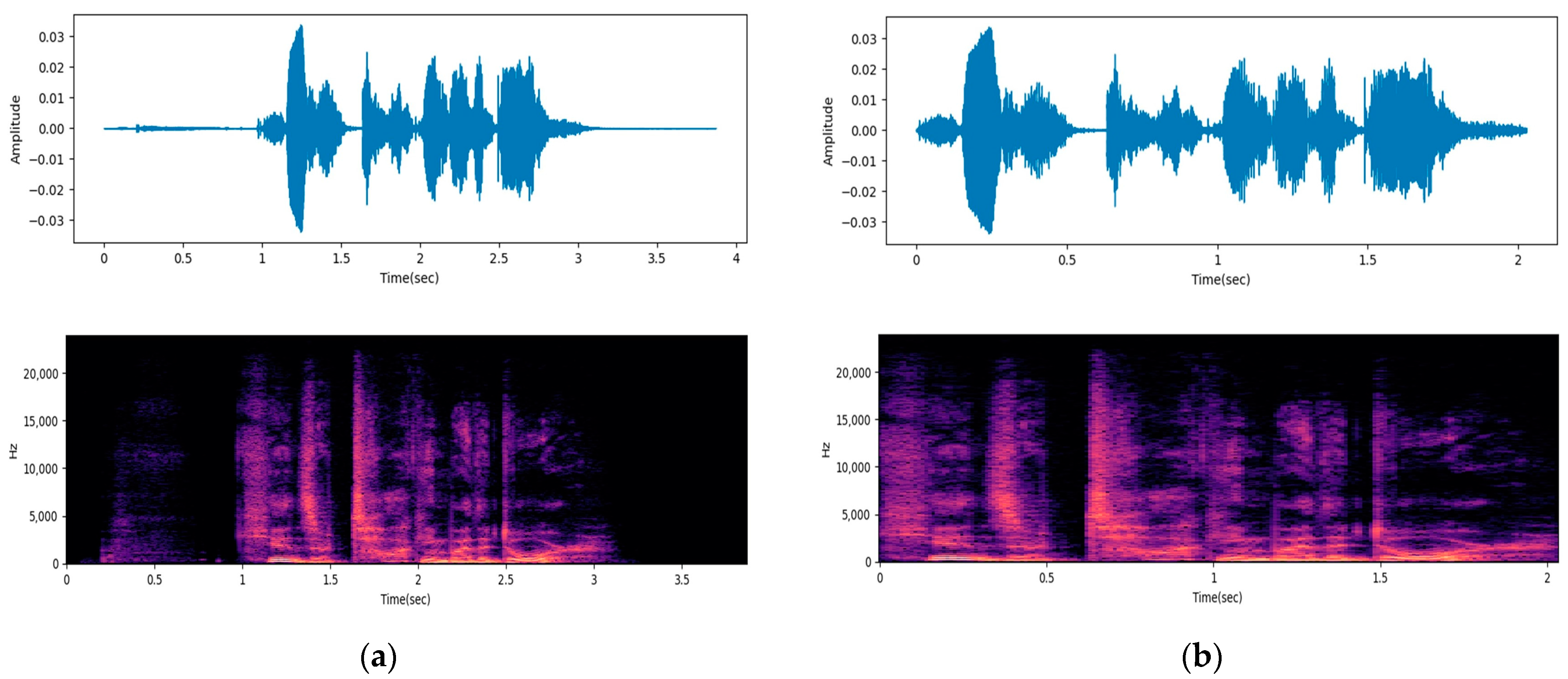
Removing non-speech segments is a crucial step in preprocessing audio data. Since Non-speech segments do not contain information related to speech information, they risk acting as noise in emotion classification. Therefore, removing such segments can contribute to the enhancement of performance in emotion recognition from speech. In this study, we utilize the effects.trim function provided in the librosa library [26] to remove non-speech segments and extract speech segments. The function works as follows. First, the amplitude envelope, which represents the amplitude of the audio signal as a function of time, is calculated to determine the change in intensity of the audio signal. Then, adaptive thresholding is performed based on the calculated amplitude envelope. If the amplitude drops below a preset threshold, it is considered a non-speech segment and removed. This process not only reduces the size of the audio data, but also makes it more suitable for emotion recognition from speech. Figure 1 shows examples of the waveforms and spectrograms before and after the removal of non-speech segments.
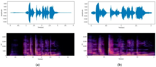
Figure 1.
Examples of preprocessing: (a) original data; (b) preprocessed data.
3.3. Feature Selection
3.3.1. Audio Features
Audio feature extraction is a key step in emotion recognition from speech. Since emotions can be expressed by the speaker’s articulation, pitch, intensity, and many other features of the voice, appropriate selection of audio features has a significant impact on the performance of emotion recognition from speech. The following audio features are considered in this study.
- MFCC, -MFCC, -MFCC: Mel-frequency cepstral coefficients (MFCC) were introduced by Davis et al. [27], and are widely used features in the field of speech recognition. The human ear does not perceive all frequencies equally, and MFCCs simulate this perception to capture the overall characteristics of speech. MFCC is a powerful audio feature that captures the unique characteristics of speech signals to enable more accurate emotion classification, and has been the centerpiece of various studies on emotion recognition from speech [28,29,30,31,32,33,34,35]. -MFCC and -MFCC are the first and second time derivatives of MFCC, which represent the dynamic characteristics of speech. In this study, 13-dimensional MFCC is extracted.
- Twelve-Dimensional Chroma Vector: Chroma vector is a feature mainly used in music analysis, which reflects the harmonic structure of speech [36]. Since the harmonic structure of speech can change depending on the expression of emotion, it can be a suitable feature for emotion recognition from speech.
- Spectral Bandwidth, Spectral Centroid, Spectral Contrast, Spectral Flatness, Spectral Rolloff [37]: These spectral features reflect the frequency domain characteristics of speech. Spectral bandwidth describes the spread of the content of the speech and typically contains information about the texture or timing of the sound. Spectral centroid represents the speaker’s tone. Spectral contrast measures the difference between the peaks and valleys of a frequency band. The difference in energy in each frequency band can reflect a particular emotional state or articulation feature of the speaker. Spectral flatness indicates how close a sound is to noise, and spectral rolloff contains information about the frequency characteristics and energy distribution of a sound.
- Root Mean Square (RMS): RMS is a feature that reflects the intensity or energy of speech, which can indicate the intensity of emotion or the activity of the speaker [38].
- Zero Crossing Rate (ZCR): ZCR refers to the frequency with which a speech signal crosses zero. The ZCR can change with emotion, with angry emotions having a particularly high ZCR.
In the following, a combination of the above audio features will be used to capture different characteristics and expressions of emotion. All features are extracted using the librosa package [26].
3.3.2. t-SNE
t-distributed Stochastic Neighbor Embedding (t-SNE) is a dimensionality reduction algorithm for visualizing the structure of high-dimensional datasets in 2D or 3D space [39]. t-SNE represents the similarity between data points as a probability distribution and maps it to a lower dimension, while preserving the maximum amount of information. It calculates the similarity between each pair of data points () in high-dimensional space using a Gaussian distribution. The similarity, , is described in Equation (1). is the probability that chooses as a neighbor. is the number of data points, and acts as a normalization constant to ensure that the sum of is equal to 1 for all pairs .
The formula for determining is presented in Equation (2), where is the standard deviation of the Gaussian distribution of data points .
The similarity of a pair of data points () mapped to a low-dimensional space is calculated as shown in Equation (3).
A cost function is then calculated to optimize the similarity in both high-dimensional and low-dimensional spaces to align as closely as possible. The cost function used in t-SNE is the Kullback–Leibler (KL) divergence. The KL divergence measures how a probability distribution diverges from a second expected probability distribution. The cost function is calculated as shown in Equation (4).
To find a configuration of points in the low-dimensional space that minimizes the KL divergence, the t-SNE is optimized via gradient descent. After computing the gradient of , the points in the low-dimensional space are updated with the aim of minimizing . The gradient descent for a single iteration t is calculated as shown in Equation (5). is the learning rate, is the gradient of the cost function with respect to . is the momentum term, which helps achieve fast and stable convergence. represents the coordinates of point in the previous iteration and corresponds to the coordinates of the point in the second last iteration.
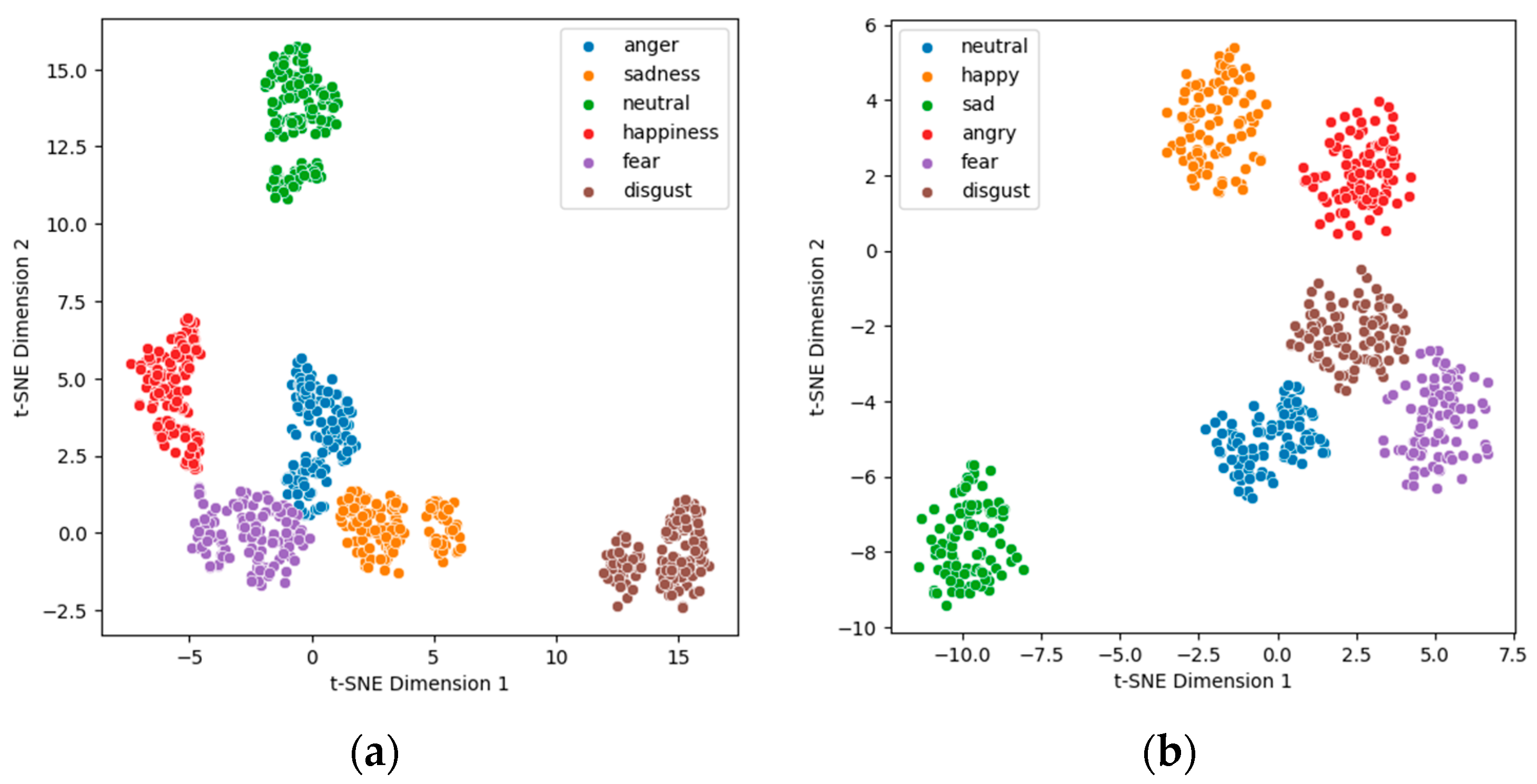
The t-SNE is useful for visually checking how effective a combination of audio features is for recognizing emotion in speech. While it is difficult to understand the distances and distributions between emotion labels in speech in a high-dimensional feature space, visualizing them in a two-dimensional space with t-SNE makes it easy to see how well each emotion category is distinguished.
In this study, 11 audio features were randomly combined and visualized with t-SNE to evaluate the effectiveness of each combination. Since clear visualization results require an equal volume of data for each emotion, we randomly selected the same number of data samples for each emotion from both the Emo-DB and RAVDESS datasets in order to perform feature vector extraction and t-SNE algorithm visualization. The feature combinations that showed the best separation for both databases were as follows.
- Emo-DB: 13MFCCs, 12Chroma Vector, Spectral Contrast, Spectral Centroid, Spectral Bandwidth, Spectral Flatness, Spectral Rolloff, RMS, ZCR.
- RAVDESS: 13MFCCs, -MFCC, Spectral Contrast, Spectral Centroid, Spectral Bandwidth, Spectral Flatness, Spectral Rolloff.Figure 2 shows a visualization of the feature combinations with the best separation in each database.
 Figure 2. t-SNE visualization: (a) Emo-DB; (b) RAVDESS.
3.4. Model
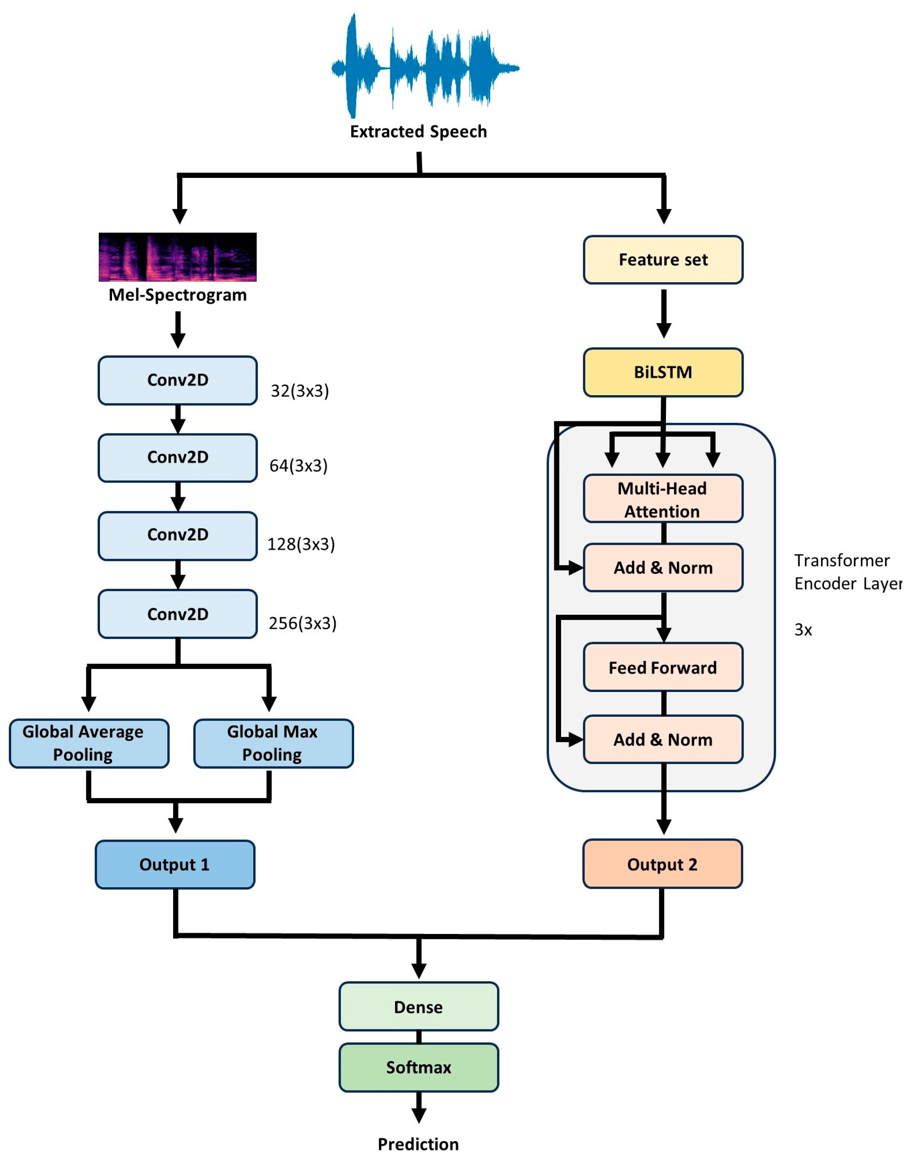
The proposed model in this study combines two main components, a 2D CNN and a BiLSTM–Transformer. The 2D CNN receives the Mel-spectrogram as input, and the BiLSTM–Transformer takes the audio features configured in Section 3.3.2 as input.
3.4.1. 2D CNN
2D CNN is designed specifically to handle the Mel-spectrogram. Mel-spectrogram is a visualized representation of time and frequency information of audio signals, and 2D CNN has a suitable structure for extracting features from image data. Therefore, the Mel-spectrogram can easily be used to detect temporal changes and frequency features, and 2D CNN can effectively learn these features. Furthermore, 2D CNN excels at recognizing local patterns. As the Mel-spectrogram reflects frequency changes in a short period of time, the features of emotional speech may be expressed in a specific time and frequency domain, and the 2D CNN can detect and learn these local patterns for emotion recognition.
3.4.2. BiLSTM–Transformer
LSTM-based models are designed to handle variable-length sequence data, which makes them well suited to working with time series data such as audio data. While LSTM processes sequence data sequentially, BiLSTM processes sequence data backwards and forwards simultaneously. This enables BiLSTM to effectively analyze past and future information in the data simultaneously. This can lead to higher accuracy in recognizing patterns.
Transformer is a model based on the attention mechanism, a technique that weights different parts of the input data to emphasize significant parts. This method proves useful in emotion recognition, as certain parts of speech that reveal emotions may hold greater importance than others. Multi-head attention is employed to capture a larger amount of information as compared to single-head attention. By using multiple “heads” to compute attention from various perspectives of the data, the multi-head attention mechanism has the ability to identify various key patterns or features at the same time. Additionally, the transformer structure facilitates parallel processing, which enables faster learning and smoother handling of large amounts of data. Since BiLSTM is effective for identifying the temporal features of audio data, and the transformer is adept at learning the complex hierarchical structures of data, the combination of these two architectures allows the model to simultaneously consider different patterns and features in audio data.
3.4.3. Preprocessing for Model Input
First, it is necessary to preprocess the data to use it as input for the 2D CNN model. Since Mel-spectrograms in audio can vary in length, it is necessary to perform a process of fitting all Mel-spectrograms to the same shape. This is achieved by first calculating the average length of the audio for each database on the basis of the extracted audio segments. Then, the length of the speech is aligned based on the value closet to the average length. The average length of Emo-DB is 2.62 s; therefore, the reference length of Emo-DB is set to 2.5 s. For RAVDESS, the average length is 2.12 s, so the reference of RAVDESS is set to 2 s. Speech data longer than the reference length are truncated at the end, while shorter speech data are lengthened by using zero padding. As a result, the same Mel-spectrogram shapes for Emo-DB (128, 79) and RAVDESS (128, 188) are used. On the other hand, the input to the BiLSTM–Transformer uses the mean value of each feature, so no additional work is required to equalize the length of the speech.
Some audio features have very different ranges or units for their values. For example, spectral contrast typically has a value of 10 units, while spectral bandwidth has a value of 1000 units. This large variation hinders the learning of the model and makes convergence more challenging, especially for gradient-based learning methods. Therefore, we normalize the values of each feature so that they have a Gaussian distribution with a mean value of 0 and a standard deviation of 1. The formula used for normalization is shown in Equation (6), where μ is the mean and σ is the standard deviation.
3.4.4. Model Architecture
The first branch is a 2D CNN, which receives the Mel-spectrogram as input. Features are extracted by passing through multiple convolutional layers, each with a ReLu activation function and L2 kernel regularization. The progression in the number of filters—32, 64, 128, and 256—ensures a hierarchical feature extraction process, with the L2 regularization of 0.001 acting as a deterrent against overfitting. The kernel size is consistently kept at (3, 3) across all convolutional layers, ensuring localized feature capture. Subsequently, the feature maps are summarized by passing them through the global average pooling and global max pooling layers, respectively. After batch normalization and a dropout rate of 0.5, the outputs from the two pooling layers are concatenated, forming a single feature vector.
The second branch is the BiLSTM–Transformer, which receives the previously configured feature set as input. The input features are first processed by a BiLSTM layer with 64 hidden units for each direction (forward and backward), resulting in a concatenated 128-dimensional output. This is then fed into the transformer layers, which consist of three transformer encoder layers, each having four attention heads. After the attention mechanism, the output passes through a dense layer with 512 units, followed by a dropout rate of 0.5 and layer normalization.
Finally, the outputs from both branches are flattened into 1D tensors. These 1D representations are then concatenated side by side, effectively merging the distinct feature representations from both branches into a unified feature vector. This combined feature vector is then further processed through a dense layer with 64 units and classified into emotion categories using the SoftMax activation function. Figure 3 illustrates the overall model.
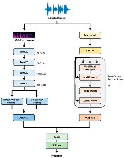
Figure 3.
BiLSTM–Transformer + 2D CNN model architecture.
4. Experiment
4.1. Evaluation Index
The 10-fold cross-validation method was used, in which the dataset was divided into 10 folds and evaluated. A total of 10% of the total data was held out and used as test data, while the remaining 90% of the data were used for training and validation. Since the training and validation data change from fold to fold during cross-validation, the performance of the model is not dependent on the specific dataset, but rather generalized.
Weighted accuracy (WA) is a measure of accuracy that takes into consideration the number of samples in each class. This is particularly significant in unbalanced datasets, because the performance of larger classes will have a greater impact on the overall performance. Unweighted accuracy (UA) is calculated by taking into consideration the accuracy of all classes equally. It is a useful means for assessing the performance of each class equally, and disregards class imbalance.
The confusion matrix is a commonly used tool for evaluating the performance of a classification model. It compares the predicted classes to the actual ones and shows how accurate the model’s predictions are. This can expose patterns, including which classes are often incorrectly predicted or which classes are commonly confused with one another.
These metrics enable the analysis of the model’s performance from various perspectives, offering direction for future model improvements.
4.2. Results
In the experiments, the model was first evaluated via 10-fold cross-validation on each dataset. A total of 10% of the data per emotion in each dataset was held out to test the model after the cross-validation process. The remaining samples were shuffled and randomly split into 10 folds of approximately equal size. Each subset k was used for validation, and the remaining subset k-1 was used to train the model. This process was repeated 10 times. The results of the accuracy validation were obtained from the 10 folds, and the average accuracy of the 10 folds was used to determine performance. The results of k-fold cross-validation are shown in Table 2. According to Table 2, the model achieved the highest recognition rate when trained on the Emo-DB dataset, with an average recognition rate of 89.06%. An average recognition rate of 70.87% was obtained on the RAVDESS dataset.
Table 2.
Ten-fold accuracy validation.
In addition, all 10 folds were tested with a 10% hold-out set. The WA and UA were calculated for the test set, and Table 3 shows the accuracy of the best-performing folds.
Table 3.
WA and UA of the best model.
Figure 4 shows the confusion matrix for the best model for each database.
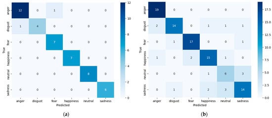
Figure 4.
Confusion matrix of the best model counts of test data: (a) Emo-DB; (b) RAVDESS.
In order to obtain an intuitive understanding of the contributions of each of the two components, BiLSTM–Transformer and 2D CNN, separate experiments were performed on each database using the 10-fold cross-validation method. Table 4 shows the unweighted accuracy of the best performing models from these individual experiments.
Table 4.
UAs of individual experiments.
These individual results accentuate the pivotal role played by each component and further emphasize their synergistic effect when combined.
Table 5 shows a comparison of the results of previous studies using the Emo-DB and RAVDESS databases with those obtained when using the LSTM and transformer models. Compared to previous studies, both Emo-DB and RAVDESS showed higher accuracy when the feature set and Mel-Spectrogram proposed for each database were used in a model in which BiLSTM–Transformer and 2D CNN were combined. This performance clearly indicates the improvement brought by our approach to the field of emotion recognition from speech. The effective combination of our chosen features and model architecture stands out when evaluated compared to existing methods.
Table 5.
Comparison of the UAs reported in previous works.
5. Conclusions
The combination of the BiLSTM–Transformer model and 2D CNN proposed in this study demonstrated superior performance at recognizing emotions from speech when compared to existing models on the RAVDESS and Emo-DB datasets, achieving recognition rates of 95% and 80.19%, respectively. These findings demonstrate a robust synergy between the bidirectional context learning capacity of BiLSTM, the attention mechanism of the transformer, and 2D CNN’s ability to capture local features in emotion recognition from speech. In particular, the combination of different architectures in the proposed model plays an important role in capturing various features and patterns of emotions.
In future research, we will expand upon the present findings to enhance the generality of the model by including other languages or larger datasets. In addition, although we focused on audio features such as MFCC, it would be possible to further improve the accuracy of the model by combining prosodic features or other audio features. Furthermore, it is essential to optimize performance by fine tuning the respective hyperparameters of BiLSTM–Transformer and 2D CNN, or by combining them with new architectures. The proposed model contributes significantly to enhancing the performance of emotion recognition from speech, and it is expected that further improvements and applications in various fields will be achieved in future research.
6. Discussion
The main idea behind combining the BiLSTM–Transformer and 2D CNN methods in this study is to bring together the best features of both approaches for emotion recognition from speech.
The 2D CNN method is well known for its ability to process images by capturing features that are close together. When we talk about speech, it can be imagined as a sort of image in which changes in sound occur over time. This image-like representation is what the 2D CNN looks at. Therefore, with 2D CNN, small and specific patterns in the speech data can be caught that are important for identifying emotions. On the other hand, speech is a sequence of sounds that happen one after the other, and understanding the order and relation of these sounds is key to recognizing emotions. This is where BiLSTM–Transformer comes in. BiLSTM looks at the speech data from both the beginning to the end and the end to the beginning, giving a fuller picture. The transformer then helps the model to focus on important parts of the speech, weighing their importance. By using both BiLSTM and the transformer, it is ensured that the model understands the full context of the speech. By combining 2D CNN with BiLSTM–Transformer, a model is obtained that can look at both specific patterns and the overall context in speech, leading to better emotion recognition.
There are several intriguing avenues for future study. One possible direction is to experiment with the data flow between the BiLSTM–Transformer and the 2D CNN. For example, the output from the BiLSTM–Transformer could be used as the input for the 2D CNN, or vice versa. This approach might lead to deeper integration between the models, maximizing the unique strengths of each. Additionally, considering a hierarchical model structure could be beneficial, where preliminary emotion categories detected by one model guide or refine the processing of the subsequent model. Furthermore, integrating a feedback loop between the 2D CNN and BiLSTM–Transformer might allow for iterative refinement. This iterative process could provide an avenue where if one model is uncertain of its prediction, insights from the other model could be used to reassess its initial assessment. Essentially, as the 2D CNN captures intricate speech patterns, its outputs could potentially be used to refine or adjust the sequence interpretations made by the BiLSTM–Transformer and vice versa, thus allowing the combined model to continuously learn and adapt with each iteration.
However, there are some areas in which our study could be improved. A notable limitation is our reliance on datasets primarily in the German and English languages. While these databases are valuable, they may not fully capture the emotional features present in other languages. By only focusing on these two languages, we may inadvertently have introduced biases or missed out on certain emotion-specific features of other languages. A direction for future research would be to incorporate databases in multiple languages. This would not only increase the diversity of the data, but also enhance the model’s capacity to generalize across varied linguistic contexts. Furthermore, conducting experiments with language-independent data, in which there is a mixture of multiple languages, could present a robust challenge and potentially drive the model to extract truly universal emotion features, rather than those tied to a specific linguistic or cultural context.
This study represents a significant step in leveraging the strengths of both the 2D CNN and BiLSTM–Transformer architectures for performing emotion recognition from speech. Our integration of these methods provides new possibilities for understanding and interpreting emotional cues in speech. While we acknowledge the limitations and areas of potential improvement, this study provides a promising foundation for future progress. As we continue to embrace a diverse range of datasets and refine our methodologies, we hold a positive outlook for developing even more advanced and widely applicable models for emotion recognition from speech in the future.
Author Contributions
Conceptualization, S.K. and S.-P.L.; methodology, S.K.; investigation, S.K.; writing—original draft preparation, S.K.; writing—review and editing, S.-P.L.; project administration, S.-P.L. All authors have read and agreed to the published version of the manuscript.
Funding
This research received no external funding.
Data Availability Statement
The experiments used publicly available datasets.
Conflicts of Interest
The authors declare no conflict of interest.
References
- Ko, B.C. A brief review of facial emotion recognition based on visual information. Sensors 2018, 18, 401. [Google Scholar] [CrossRef] [PubMed]
- Canal, F.Z.; Müller, T.R.; Matias, J.C.; Scotton, G.G.; de Sa Junior, A.R.; Pozzebon, E.; Sobieranski, A.C. A survey on facial emotion recognition techniques: A state-of-the-art literature review. Inf. Sci. 2022, 582, 593–617. [Google Scholar] [CrossRef]
- Valstar, M.; Pantic, M. Fully automatic facial action unit detection and temporal analysis. In Proceedings of the IEEE 2006 Conference on Computer Vision and Pattern Recognition Workshop (CVPRW’06), New York, NY, USA, 17–22 June 2006; p. 149. [Google Scholar]
- Burkhardt, F.; Paeschke, A.; Rolfes, M.; Sendlmeier, W.F.; Weiss, B. A database of German emotional speech. Interspeech 2005, 5, 1517–1520. [Google Scholar]
- De Lope, J.; Graña, M. An ongoing review of speech emotion recognition. Neurocomputing 2023, 528, 1–11. [Google Scholar] [CrossRef]
- Vaswani, A.; Shazeer, N.; Parmar, N.; Uszkoreit, J.; Jones, L.; Gomez, A.N.; Kaiser, Ł.; Polosukhin, I. Attention is all you need. In Proceedings of the Advances in Neural Information Processing Systems, Long Beach, CA, USA, 4–9 December 2017; Volume 30. [Google Scholar]
- Issa, D.; Demirci, M.F.; Yazici, A. Speech emotion recognition with deep convolutional neural networks. Biomed. Signal Process. Control 2020, 59, 101894. [Google Scholar] [CrossRef]
- Mocanu, B.; Tapu, R. Emotion recognition from raw speech signals using 2d cnn with deep metric learning. In Proceedings of the 2022 IEEE International Conference on Consumer Electronics (ICCE), Las Vegas, NV, USA, 22–28 October 2022; pp. 1–5. [Google Scholar]
- Lim, W.; Jang, D.; Lee, T. Speech emotion recognition using convolutional and recurrent neural networks. In Proceedings of the IEEE 2016 Asia-Pacific Signal and Information Processing Association Annual Summit and Conference (APSIPA), Jeju, Republic of Korea, 13–15 December 2016; pp. 1–4. [Google Scholar]
- Anvarjon, T.; Mustaqeem; Kwon, S. Deep-net: A lightweight CNN-based speech emotion recognition system using deep frequency features. Sensors 2020, 20, 5212. [Google Scholar] [CrossRef]
- Parry, J.; Palaz, D.; Clarke, G.; Lecomte, P.; Mead, R.; Berger, M.; Hofer, G. Analysis of Deep Learning Architectures for Cross-Corpus Speech Emotion Recognition. In Proceedings of the Interspeech, Graz, Austria, 15–19 September 2019; pp. 1656–1660. [Google Scholar]
- Kerkeni, L.; Serrestou, Y.; Mbarki, M.; Raoof, K.; Mahjoub, M.A.; Cleder, C. Automatic Speech Emotion Recognition Using Machine Learning; IntechOpen: London, UK, 2019. [Google Scholar]
- Devlin, J.; Chang, M.-W.; Lee, K.; Toutanova, K. Bert: Pre-training of deep bidirectional transformers for language understanding. arXiv 2018, arXiv:1810.04805. [Google Scholar]
- Radford, A.; Wu, J.; Child, R.; Luan, D.; Amodei, D.; Sutskever, I. Language models are unsupervised multitask learners. OpenAI blog 2019, 1, 9. [Google Scholar]
- Yang, Z.; Dai, Z.; Yang, Y.; Carbonell, J.; Salakhutdinov, R.R.; Le, Q.V. Xlnet: Generalized autoregressive pretraining for language understanding. In Proceedings of the Advances in Neural Information Processing Systems, Vancouver, BC, Canada, 8–14 December 2019; Volume 32. [Google Scholar]
- Beltagy, I.; Peters, M.E.; Cohan, A. Longformer: The long-document transformer. arXiv 2020, arXiv:2004.05150. [Google Scholar]
- Brown, T.; Mann, B.; Ryder, N.; Subbiah, M.; Kaplan, J.D.; Dhariwal, P.; Neelakantan, A.; Shyam, P.; Sastry, G.; Askell, A. Language models are few-shot learners. Adv. Neural Inf. Process. Syst. 2020, 33, 1877–1901. [Google Scholar]
- Heusser, V.; Freymuth, N.; Constantin, S.; Waibel, A. Bimodal speech emotion recognition using pre-trained language models. arXiv 2019, arXiv:1912.02610. [Google Scholar]
- Lee, S.; Han, D.K.; Ko, H. Fusion-ConvBERT: Parallel convolution and BERT fusion for speech emotion recognition. Sensors 2020, 20, 6688. [Google Scholar] [CrossRef] [PubMed]
- Jing, D.; Manting, T.; Li, Z. Transformer-like model with linear attention for speech emotion recognition. J. Southeast Univ. 2021, 37, 164–170. [Google Scholar]
- Dai, Z.; Yang, Z.; Yang, Y.; Carbonell, J.; Le, Q.V.; Salakhutdinov, R. Transformer-xl: Attentive language models beyond a fixed-length context. arXiv 2019, arXiv:1901.02860. [Google Scholar]
- Sakatani, Y. Combining RNN with Transformer for Modeling Multi-Leg Trips. In Proceedings of the WebTour@ WSDM, Jerusalem, Israel, 12 March 2021; pp. 50–52. [Google Scholar]
- Text Generation With LSTM+Transformer Model. Available online: https://note.com/diatonic_codes/n/nab29c78bbf2e (accessed on 22 April 2020).
- Andayani, F.; Theng, L.B.; Tsun, M.T.; Chua, C. Hybrid LSTM-transformer model for emotion recognition from speech audio files. IEEE Access 2022, 10, 36018–36027. [Google Scholar] [CrossRef]
- Livingstone, S.R.; Russo, F.A. The Ryerson Audio-Visual Database of Emotional Speech and Song (RAVDESS): A dynamic, multimodal set of facial and vocal expressions in North American English. PLoS ONE 2018, 13, e0196391. [Google Scholar] [CrossRef] [PubMed]
- McFee, B.; Matt, M.; Daniel, F.; Iran, R.; Matan, G.; Stefan, B.; Scott, S.; Ayoub, M.; Colin, R.; Vincent, L.; et al. Librosa/librosa, version 0.10.1; Zenodo: Geneva, Switzerland, 2023. [Google Scholar]
- Davis, S.; Mermelstein, P. Comparison of parametric representations for monosyllabic word recognition in continuously spoken sentences. IEEE Trans. Acoust. Speech Signal Process. 1980, 28, 357–366. [Google Scholar] [CrossRef]
- Chen, L.; Mao, X.; Xue, Y.; Cheng, L.L. Speech emotion recognition: Features and classification models. Digit. Signal Process. 2012, 22, 1154–1160. [Google Scholar] [CrossRef]
- Dahake, P.P.; Shaw, K.; Malathi, P. Speaker dependent speech emotion recognition using MFCC and Support Vector Machine. In Proceedings of the 2016 IEEE International Conference on Automatic Control and Dynamic Optimization Techniques (ICACDOT), Pune, India, 9–10 September 2016; pp. 1080–1084. [Google Scholar]
- Daneshfar, F.; Kabudian, S.J.; Neekabadi, A. Speech emotion recognition using hybrid spectral-prosodic features of speech signal/glottal waveform, metaheuristic-based dimensionality reduction, and Gaussian elliptical basis function network classifier. Appl. Acoust. 2020, 166, 107360. [Google Scholar] [CrossRef]
- Gao, Y.; Li, B.; Wang, N.; Zhu, T. Speech emotion recognition using local and global features. In Proceedings of the Brain Informatics: International Conference, BI 2017, Beijing, China, 16–18 November 2017; Springer: Berlin/Heidelberg, Germany, 2017; pp. 3–13. [Google Scholar]
- Kishore, K.K.; Satish, P.K. Emotion recognition in speech using MFCC and wavelet features. In Proceedings of the 2013 3rd IEEE International Advance Computing Conference (IACC), Ghaziabad, India, 22–23 February 2013; pp. 842–847. [Google Scholar]
- Milton, A.; Roy, S.S.; Selvi, S.T. SVM scheme for speech emotion recognition using MFCC feature. Int. J. Comput. Appl. 2013, 69, 34–39. [Google Scholar] [CrossRef]
- Praseetha, V.; Vadivel, S. Deep learning models for speech emotion recognition. J. Comput. Sci. 2018, 14, 1577–1587. [Google Scholar] [CrossRef]
- Zamil, A.A.A.; Hasan, S.; Baki, S.M.J.; Adam, J.M.; Zaman, I. Emotion detection from speech signals using voting mechanism on classified frames. In Proceedings of the 2019 International Conference on Robotics, Electrical and Signal Processing Techniques (ICREST), Dhaka, Bangladesh, 10–12 January 2019; pp. 281–285. [Google Scholar]
- Muller, M.; Ellis, D.P.; Klapuri, A.; Richard, G. Signal processing for music analysis. IEEE J. Sel. Top. Signal Process. 2011, 5, 1088–1110. [Google Scholar] [CrossRef]
- Peeters, G. A large set of audio features for sound description (similarity and classification) in the CUIDADO project. CUIDADO Ist Proj. Rep. 2004, 54, 1–25. [Google Scholar]
- Giannoulis, D.; Benetos, E.; Stowell, D.; Rossignol, M.; Lagrange, M.; Plumbley, M.D. Detection and classification of acoustic scenes and events: An IEEE AASP challenge. In Proceedings of the 2013 IEEE Workshop on Applications of Signal Processing to Audio and Acoustics, New Paltz, NY, USA, 20–23 October 2013; pp. 1–4. [Google Scholar]
- Van der Maaten, L.; Hinton, G. Visualizing data using t-SNE. J. Mach. Learn. Res. 2008, 9, 2579–2605. [Google Scholar]

Disclaimer/Publisher’s Note: The statements, opinions and data contained in all publications are solely those of the individual author(s) and contributor(s) and not of MDPI and/or the editor(s). MDPI and/or the editor(s) disclaim responsibility for any injury to people or property resulting from any ideas, methods, instructions or products referred to in the content. |
© 2023 by the authors. Licensee MDPI, Basel, Switzerland. This article is an open access article distributed under the terms and conditions of the Creative Commons Attribution (CC BY) license (https://creativecommons.org/licenses/by/4.0/).