Broadband Modelling of Power Transformers for Sweep Frequency Impedance Studies on Winding Short-Circuit Faults

Abstract

To study sweep frequency impedance (SFI) features of short-circuit (SC) faults easily, this paper proposes a broadband electric circuit model of a transformer winding and solves its three key problems. The first problem is the calculation of lumped-circuit parameters considering frequency-dependent complex anisotropic permeabilities (FDCAPs), which are caused by the physical characteristics, such as skin, proximity, and geometrical effects and anisotropic properties, of the transformer core and winding materials. The other issue is the establishment of the electric circuit model based on the SFI measurement connection mode, the transformer winding parameters, and a double-ladder network (DLN). Another issue is the construction of the state-space model of the electric circuit toward different SFI values to obtain all network branch voltages and currents. The accuracy of the proposed model is assessed by comparing its SFI signatures with those of the simulation model, without considering FDCAPs under healthy winding, and the corresponding physical transformer model during healthy winding and SC faults. It is observed that the SFI results of the proposed model are closer to the experimental measurements, and the model can be effectively used to study the SFI features of SC faults. Moreover, the impacts of different types of SC faults on the SFI data are concluded in this paper.

1. Introduction

Power transformers are some of the most crucial apparatuses in power systems, which are used to transfer electrical energy through electromagnetic induction [1,2,3]. They are vulnerable to mechanical changes during their lifetimes, which typically manifest as winding deformation, such as shorted or open turns, axial displacement, conductor tilting, radial displacement, and so on [4,5]. Among the major problems, a potential short-circuit (SC) fault between winding turns or discs can cause great harm to the stable operation of the transformer [6]. It continually decreases longitudinal insulation between adjacent turns and finally leads to catastrophic damage to the transformer. Therefore, the development of a precise diagnostic method for SC faults is one of the most important aspects of transformer condition monitoring.

Frequency response analysis (FRA), short-circuit impedance (SCI), and sweep frequency impedance (SFI) have been widely used to detect SC faults of transformer windings [7,8,9,10]. Compared to the first two, SFI has a greater signal-to-noise ratio, better repeatability, and more affluent information related to winding mechanical conditions [9,11]. This method relies on the variation of the SFI signature to judge whether or not mechanical changes occur on a transformer winding [9]. Hence, to detect an SC fault within a transformer accurately, it is significant to understand the corresponding SFI signatures of SC faults with different levels and at different positions of a transformer winding. At present, SFI signatures of winding deformation are mainly studied using an experimental method, in which winding deformation is simulated by manufacturing mechanical faults on windings artificially [9,12]. However, the method is time-consuming and high-cost, as well as difficult to apply in a large-scale power transformer.

To solve the abovementioned problem, the majority of these studies have been performed via simulation analysis based on FEM [13], mathematical modelling [14], and equivalent electric circuit models. The latter can be further divided into ladder network equivalent models [3,7], multiconductor transmission line models [15], and hybrid models [16]. Among these models, a combination of FEM modelling and ladder network modelling with lumped parameters has been widely used in simulation studies of winding deformation [5,13,17,18,19,20,21,22]. Although establishing a detailed lumped-parameter circuit model is essential to extract the accurate response features of deformed windings, most of the abovementioned studies, such as [13,17,18,19,20], did not consider the influences of frequency-dependent complex anisotropic permeabilities (FDCAPs), caused by the physical characteristics (e.g., skin, proximity, and geometrical effects and anisotropic properties) of the core and winding materials, on the lumped parameters of winding equivalent circuits. These result in an inaccurate trend of the obtained curve signature that can emulate the practical signature of a real transformer. Differently, in [5,21,22], the aforementioned influencing factors had been introduced in the calculation of circuit lumped parameters, but the established FEM model calculating the parameters was not the three-phase transformer used widely in a power grid. Moreover, considering different connection modes and theories of FRA and SFI measurements [9], the circuit models based on FRA measurement in [5,13,17,18,19,20,21,22] are also not suitable for SFI studies. Therefore, it is extremely crucial to establish a circuit model relating to the integral winding structure of the three-phase transformer and the FDCAPs of SFI measurements for accurate studies on the SFI features of SC faults.

In this paper, a broadband circuit model based on the SFI test principle, transformer winding parameters, and a double-ladder network (DLN) is proposed to investigate the SFI signatures of SC faults. The winding parameters were calculated using a FEM model, considering the FDCAPs of the core and winding materials, of a three-phase transformer. Experiments were carried out on an equivalent transformer hardware model with continuous windings specially made for this research. The correctness of the proposed model was verified by comparing its SFI signature with those of a simulation model without considering FDCAPs, and the hardware model. In addition, through experimental measurements and simulation analyses, it was proved that using the model to obtain the SFI features of SC faults is feasible, and the SFI features of different types of SC faults were studied and summarized. Considering that SFI is a comparative method using graphical inspection or statistical indicators, the modelling method proposed in this paper can assist in facilitating the objective and quantitative interpretation of transformer SFI results and provide a new way to crack the challenge of studying transformer inner winding deformation.

In summary, the contributions of this paper are listed as follows:

• Calculating the frequency-dependent lumped inductance and resistance by using the FEM model, considering the FDCAPs of core and winding materials, of the three-phase transformer to improve the accuracy of simulation;
• A circuit model and its state equations are proposed to simulate SFI measurements for studies on the SFI signatures of winding SC faults, which could offer a new practicable idea for SFI method interpretation;
• The SFI data obtained from the proposed modelling method are compared with those of other methods (e.g., experimental measurements, and a modelling method, without considering FDCAPs) to show its effectiveness and superiority;
• Providing the SFI characteristics of SC faults at different levels and different positions, especially the fault occurring on a non-tested winding, by a comparison of the experiment and simulation to set a foundation for the detection of SC faults.

The rest of this paper is organized as follows: Section 2 introduces the investigated transformer and the SFI measurement procedure. The FEM modelling and winding parameters are presented in Section 3. Section 4 introduces the proposed modelling method of SFI. The results of the simulation and experiment are presented in Section 5. Section 6 presents the conclusions of this paper.

2. Test Objects and Measurements

2.1. Test Objects

The voltage level of the measured transformer is 10 kV in this paper, and its high-voltage (HV) and low-voltage (LV) windings are both continuous disc-type structures. To change the connection group and failure form of the windings easily, the heads and terminals of the three-phase windings are placed in the bushings above the transformer tank, and the taps are set on the outer side of each winding disc, as shown in Figure 1. The main specifications of this transformer are listed in

Table 1. Transformer specifications.

Type	Value	Type	Value
Rated voltage	10/0.38 kV	Number of phases	3
Rated power	50 kVA	Frequency	50 Hz
Rated current	2.88/75.9 A	Cooling system	ONAN
Length of tank	1073 mm	Height of LV winding	501 mm
Width of tank	492 mm	External radius of LV winding	76 mm
Height of tank	940 mm	Interradius of LV winding	68.5 mm
Height of HV winding	507 mm	Number of HV winding discs	49
External radius of HV winding	164 mm	Number of LV winding discs	52
Interradius of HV winding	92 mm

.

2.2. SFI Measurements

The connections and instruments of the SFI measurements are shown in Figure 2, which include a high-speed data acquisition device, a broadband signal generator, a power amplifier, and a measured transformer.

In SFI measurements, the non-tested side of one-phase windings within a transformer is shorted. To avoid the impacts of non-defect factors on SFI data at high frequencies, the frequency range of the sinusoidal signal, loaded on the head of the tested winding, is generally limited between 10 Hz and 1 MHz [9]. The excitation signal, U_in (the bold italic letter stands for vectors), and the response, U_out, are acquired by the resistors, R₁ and R₂, respectively. The SFI value of the tested winding, namely, Z, is obtained according to:

$$Z=\left|\frac{U_{in}-U_{out}}{I_1}\right|;\hspace{1em}\hspace{0.17em}{I}_1=\frac{U_{out}}{R_2}.$$

(1)

Then, Equation (1) is transformed as:

$$Z=R_2\sqrt{{\left(\frac{U_{in}}{U_{out}}\right)}^2-2\left(\frac{U_{in}}{U_{out}}\right)\cos ({\theta }_{in}-{\theta }_{out})+1}.$$

(2)

In (2), U_in and U_out are the amplitudes of the drive signal, U_in, and the response signal, U_out, respectively. Similarly, θ_in and θ_out are the phases of U_in and U_out. To easily observe and compare the difference between the SFI signatures of healthy and faulted windings, SFI data are usually expressed in the logarithm form, which is written as [9]:

$$Z_k=20\times {\log }_{10}\left(Z\right),$$

(3)

where the unit of Z_k is defined as dBΩ. Any type of winding deformation could be reflected as a corresponding variation in SFI traces. Moreover, the deviation of the SFI value, Z, at 50 Hz, calculated with (4), can be used as a statistical index to detect a mechanical deformation on a transformer winding.

$$\Delta Z=100\%\times \left|\frac{Z_{\mathit{measurement}}-Z_{\mathit{fingerprint}}}{Z_{\mathit{fingerprint}}}\right|,$$

(4)

where Z_measurement and Z_fingerprint are the SFI measurement and its fingerprint values, respectively. An index of more than 3% indicates that a winding deformation exists in the transformer [9].

3. FEM Modelling of Winding Parameters

Figure 1 and Figure 2 show that a detailed SFI simulation circuit model should include capacitive, inductive, conductive, and resistive parameters to reflect the measurement connection and winding mechanical state. The circuit parameters, reflecting the winding mechanical state, are generally calculated using mathematical analysis and FEM modelling, but the latter is more suitable for extracting the circuit parameters of a transformer with a complex structure. Therefore, FEM modelling was applied to calculate the circuit parameters of the transformer in Figure 1.

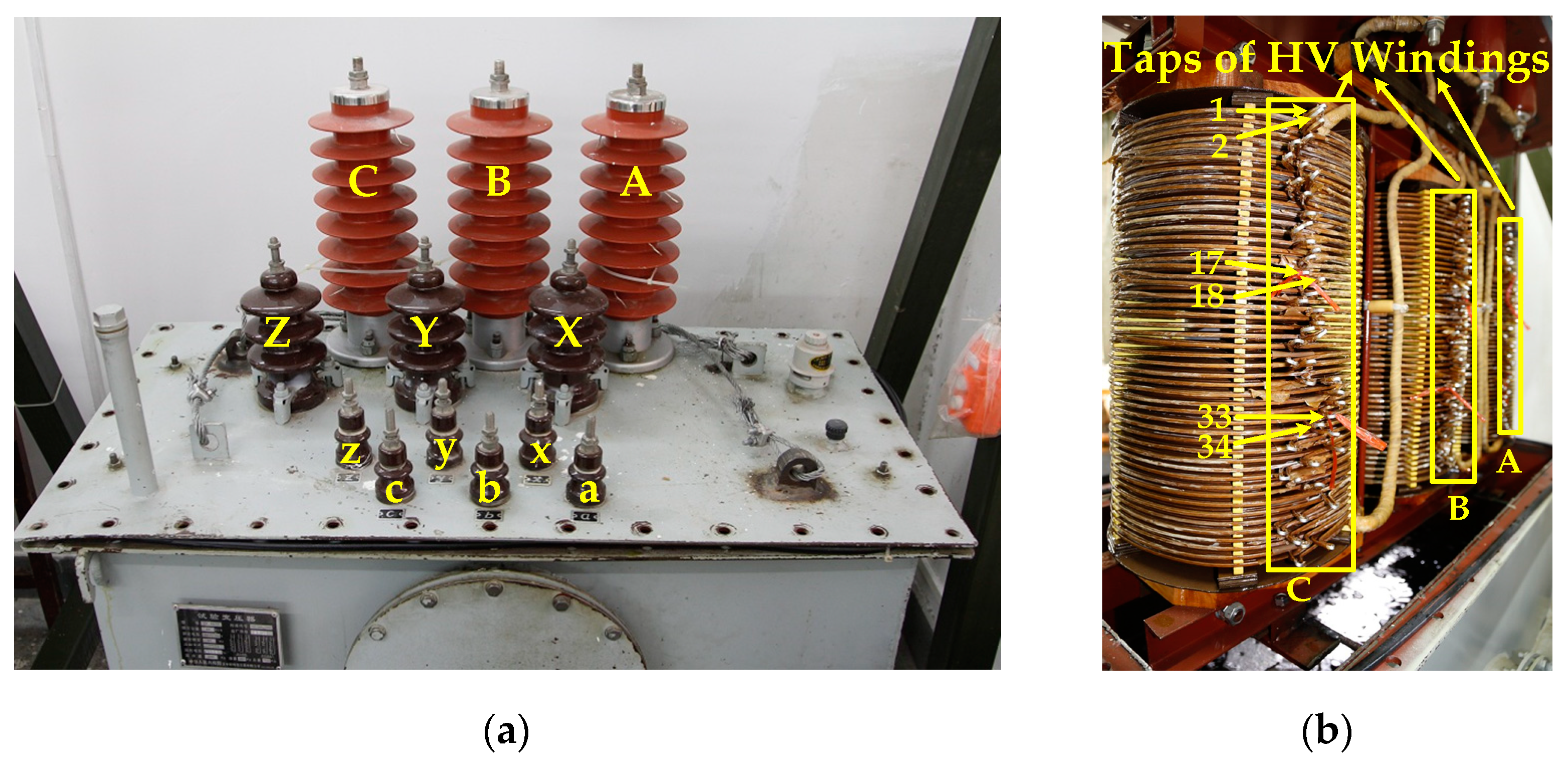
Based on the specifications of the investigated transformer in Table 1, the FEM model (see Figure 3) of the transformer was established to calculate the parameters of the C-phase windings, which include the inductance, capacitance, resistance, and conductance of each winding disc. The FEM model was composed of a transformer tank, three-phase HV and LV windings, a laminated magnetic iron core, and insulating oil.

Considering the computational accuracy and time of the model comprehensively, both the phase A and B windings were simplified as hollow cylinders, though not the phase C windings, and the total FEM model could be set as one-half of the transformer on account of its symmetrical structure. Therefore, the parameters obtained from the FEM model needed to be multiplied by two when they were applied in the circuit model.

In this paper, to extract the SFI feature of a transformer winding accurately, the inductances and resistances, calculated using the FEM model, needed to consider FDCAPs. However, the skin effect at high frequencies could lead to a longer simulation time due to increased meshing elements. To solve the problem, the FEM model in the magnetostatic mode was used to replace that in the frequency-domain mode. The detailed calculation procedures of the winding parameters are written as follows.

3.1. Inductance and Resistance

The computational domains of the FEM model in Figure 3, namely, Ω₁, Ω₂, Ω₃, and Ω₄, represent the volumes of the HV windings, LV windings, insulation oil, and core, respectively. The suitable boundary conditions are applied as zero normal components of magnetic-field intensity (n·Ĥ = 0, where n denotes the surface normal and Ĥ is the magnetic-field intensities through the surface) on the outer external boundaries and a zero tangential component of the magnetic field (n × Ĥ = 0) on the tangent plane. The permeabilities of Ω₁, Ω₂, Ω₃, and Ω₄ are, respectively, ${\overleftrightarrow{\widehat{\mu }}}_{HV}$, ${\overleftrightarrow{\widehat{\mu }}}_{LV}$, ${\mu }_{IO}$, and ${\overleftrightarrow{\widehat{\mu }}}_{core}$, which can be obtained via FEM modelling and mathematical analysis, as shown in Figure 4. Additionally, the above symbols ^ and ↔ are used to represent complex quantities and tensors, respectively.

The calculation procedure for the permeabilities is described as follows:

• The permeabilities of HV and LV windings are primarily affected by skin, geometrical, and proximity effects and the anisotropy of conductors, so a 2-D axisymmetric FEM model is implemented using an eddy current solver to obtain the FDCAPs (${\overleftrightarrow{\widehat{\mu }}}_{HV}$ and ${\overleftrightarrow{\widehat{\mu }}}_{LV}$) of the conductors on the computational domains Ω₁ and Ω₂ [22];
• Since the insulation oil is a nonmagnetic material, the permeability, ${\mu }_{IO}$, of domain Ω₃ is always equal to the vacuum permeability at different frequencies;
• Considering the skin effect and anisotropy of the silicon steel sheet, the effective FDCAP, ${\overleftrightarrow{\widehat{\mu }}}_{core}$, of Ω₄ in Figure 4 is divided into X, Y, and Z directions, and they can be expressed as [21]:

  $${\widehat{\mu }}_x^{eff}={\mu }_x^{\prime }-j{\mu }_x^{″}=k_{fe}{\mu }_x\frac{\tanh \left(\left(1+j\right)b/{\delta }_x\right)}{\left(\left(1+j\right)b/{\delta }_x\right)};\delta =\sqrt{\frac{2}{\left(\omega \sigma {\mu }_0{\mu }_x\right)}},$$

  (5)

  $${\widehat{\mu }}_y^{eff}={\mu }_y^{\prime }-j{\mu }_y^{″}=k_{fe}{\mu }_y\frac{\tanh \left(\left(1+j\right)b/{\delta }_y\right)}{\left(\left(1+j\right)b/{\delta }_y\right)};{\delta }_y=\sqrt{\frac{2}{\left(\omega \sigma {\mu }_0{\mu }_y\right)}},$$

  (6)

  and

  $${\widehat{\mu }}_z^{eff}={\mu }_z/\left[{\mu }_z\left(1-k_{fe}\right)+k_{fe}\right],$$

  (7)

  where δ_x and δ_y are, respectively, the skin depths in the X and Y directions; ω is the angular frequency; μ₀ is the vacuum permeability; σ is the conductivity of the silicon steel sheet; and k_fe is the stacking factor of the core, which can be derived by k_fe = 2b/h (h and 2b are the mean thicknesses of a single lamination of the core with and without an insulation layer, respectively). In [23], it is indicated that the magnetic permeability of the paramagnetic direction is about two times more than that of the non-paramagnetic direction in the anisotropic silicon steel sheet. Therefore, the relative permeability relationship of the silicon steel sheet in the X, Y, and Z directions can be written as μ_y = μ_z = μ_x/2. The following parameters are used in the computation of the core permeability: μ_x = 5.5 × 10³, μ_y = μ_z = μ_x/2 = 2.75 × 10³, σ = 6 × 10⁷ S/m, b = 3 × 10^–4 m, and h = 6.5 × 10^–4 m.

After assigning the abovementioned frequency-dependent permeabilities of the different computational domains in the 3-D FEM transformer model, an external alternating current, Î, is injected into the ith disc of the winding. Then, the transformer model with the healthy windings is divided into 344,918 mesh elements, as illustrated in Figure 5a, and its parameters of the magnetic field with permeabilities of different frequencies are solved using a magnetostatic solver. Figure 5b,c illustrate the simulation results of magnetic fluxes at 50 Hz and 1 MHz, respectively, in which the arrows and color shades indicate the distribution and magnitude of magnetic fluxes. From the figures, the magnetic fluxes at 50 Hz converge in the core, and at 1 MHz they are mainly located in the insulating material. Since the inductances and resistances in the circuit model are derived from the magnetic fluxes of the transformer, the impacts of the FDCAPs, caused by the skin, proximity, and geometrical effects and anisotropic properties, of the transformer core and winding on inductances and resistances at different frequencies are very obvious. This indicates that the FDCAPs cannot be ignored in establishing an accurate SFI measurement model.

Based on the induced voltages calculated in the FEM model at different frequencies, the frequency-dependent self-inductance, L_ii, and self-resistance, R_ii, of the ith winding disc could be extracted, which are defined as:

$$L_{ii}=\frac{1}{\omega }\mathrm{Im}\left(\frac{{\widehat{U}}_i}{\widehat{I}}\right),R_{ii}=\mathrm{Re}\left(\frac{{\widehat{U}}_i}{\widehat{I}}\right),$$

(8)

and the frequency-dependent mutual inductance, M_ij, and mutual resistance, R_ij, between the ith and jth discs can be derived by:

$$M_{ij}=\frac{1}{\omega }\mathrm{Im}\left(\frac{{\widehat{U}}_j}{\widehat{I}}\right),R_{ij}=\mathrm{Re}\left(\frac{{\widehat{U}}_j}{\widehat{I}}\right),$$

(9)

where ${\widehat{U}}_i$ and ${\widehat{U}}_j$ are, respectively, the induced voltages in the ith and jth winding discs. They can be calculated using (10):

$${\widehat{U}}_i=\frac{N_i}{S_{ci}}j\omega {\displaystyle {\int }_{{\Omega }_i}{\widehat{A}}_i\cdot t_i}d\Omega ,{\widehat{U}}_j=\frac{N_j}{S_{cj}}j\omega {\displaystyle {\int }_{{\Omega }_j}{\widehat{A}}_j\cdot t_j}d\Omega .$$

(10)

Here, ${\widehat{A}}_i$ and ${\widehat{A}}_j$ and $t_i$ and $t_j$ are, respectively, the magnetic vector potentials and the unit vectors in the azimuthal direction of the ith and jth discs; and N_i and N_j, S_ci and S_cj, and Ω_i and Ω_j are the turn numbers, total cross-sectional areas, and computational domains of the two winding discs, respectively [22].

As the order of the inductance and resistance matrices is huge, just some frequency-dependent inductances and resistances of the first disc on the HV winding of phase C are plotted in Figure 6. From the figures, as the frequency increases, the inductances and resistances of the first winding disc show decreasing and increasing trends, respectively. From 10 Hz to 1 MHz, the ratio between the maximum and the minimum of the inductance is 400, and that of the resistance can reach as high as 2000.

Summarily, to study SFI signatures of winding deformation through simulation analysis accurately, the FDCAPs should be considered in the calculation of the inductances and resistances.

3.2. Capacitance and Conductance

The capacitances and conductances of the transformer FEM model can be calculated using the net charge, Q, in the electrostatic field mode. The transformer model in Figure 3 can be regarded as a system with n electrodes (i.e., transformer winding discs) and one grounding (including the tank and the core), and its insulating material permittivity is set as that of free space. Therefore, the charge matrix, Q, of the winding discs in the transformer model can be derived as:

$$Q=\left[\begin{array}{c}{Q}_1\\ ⋮\\ Q_i\\ ⋮\\ Q_n\end{array}\right]=\left[\begin{array}{ccccc}{C}_{11}^g& \cdots & C_{1i}^g& \cdots & C_{1n}^g\\ ⋮& \ddots & ⋮& \ddots & ⋮\\ C_{i1}^g& \cdots & C_{ii}^g& \cdots & C_{in}^g\\ ⋮& \ddots & ⋮& \ddots & ⋮\\ C_{n1}^g& \cdots & C_{ni}^g& \cdots & C_{nn}^g\end{array}\right]\left[\begin{array}{c}{U}_1\\ ⋮\\ U_i\\ ⋮\\ U_n\end{array}\right]=C_{g}U,$$

(11)

where Q_i is the charge quantity in the ith disc winding, $C_{ij}^g$ stands for the Maxwell capacitance between the ith disc and the jth disc, and U_i represents the voltage of the ith disc.

When the voltages of the tank and core are both ground potential, and the voltages of the first disc of the phase C HV winding and the other windings are 1 V and 0 V, respectively, the capacitances (e.g., $C_{11}^g$, …, $C_{n1}^g$) related to the first disc could be given by (11). Similarly, the capacitances of the other discs could also be calculated. Figure 7 shows an example of the simulation results, which illustrates the electrical potential distribution and the setting of the FEM model in the calculation of the capacitances and conductances for the first disc.

However, the Maxwell capacitance matrix, C_g, calculated in (11) cannot be directly implemented in the circuit, which should be transformed into the lumped capacitance matrix, C_d, as follows [17]:

$$C_d=\left[\begin{array}{ccccc}{\displaystyle \sum _{j=1}^n{C}_{1j}^g}& \cdots & -C_{1i}^g& \cdots & -C_{1n}^g\\ ⋮& \ddots & ⋮& \ddots & ⋮\\ -C_{i1}^g& \cdots & {\displaystyle \sum _{j=1}^n{C}_{ij}^g}& \cdots & -C_{in}^g\\ ⋮& \ddots & ⋮& \ddots & ⋮\\ -C_{n1}^g& \cdots & -C_{ni}^g& \cdots & {\displaystyle \sum _{j=1}^n{C}_{nj}^g}\end{array}\right].$$

(12)

The capacitance matrix, C, and conductance matrix, G, used in the circuit model can be derived as:

$$C={\epsilon }_r^{\prime }{C}_d,G=\omega {\epsilon }_r^{″}{C}_d,$$

(13)

where ${\epsilon }_r^{\prime }$ and ${\epsilon }_r^{″}$ are the real and imaginary parts of the relative permittivity of the insulating material, respectively. Considering that the insulating oil accounts for about 100% of the total transformer insulation materials, the relative complex permittivity of the insulating oil is taken as that of the whole insulating material in the transformer, which can be written as [18]:

$${\widehat{\epsilon }}_r\left(\omega \right)={\epsilon }_r^{\prime }-\mathrm{j}{\epsilon }_r^{″}=2.2-\mathrm{j}\frac{{\sigma }_{in}}{{\epsilon }_0\omega },$$

(14)

where ε₀ is the permittivity of free space, σ_in is the conductivity of the insulation oil, and its value is 2.05 × 10^–12 S/m. Similar to the inductance and resistance matrices, the order of the capacitance and conductance matrices of the FEM model is also very big, so

Table 2. Some capacitances and conductances of the upper three discs for the phase C HV winding from 10 Hz to 1 MHz.

Parameter Type and Unit	Parameter	Value	Parameter	Value	Parameter	Value
Capacitance/pF	C1,1	34.29	C1,2	174.21	C1,50	6.62
	C2,2	4.44	C2,3	171.91	C2,51	2.45
	C3,3	3.79	C3,4	172.99	C3,52	2.42
Conductance/nS	G1,1	3.61	G1,2	18.34	G1,50	0.70
	G2,2	0.47	G2,3	18.10	G2,51	0.26
	G3,3	0.40	G3,4	18.21	G3,52	0.25

just lists the ground capacitances and conductances of the upper three discs for the phase C HV winding and their mutual capacitances and conductances with adjacent discs (see Figure 3).

4. Modelling of SFI Measurements

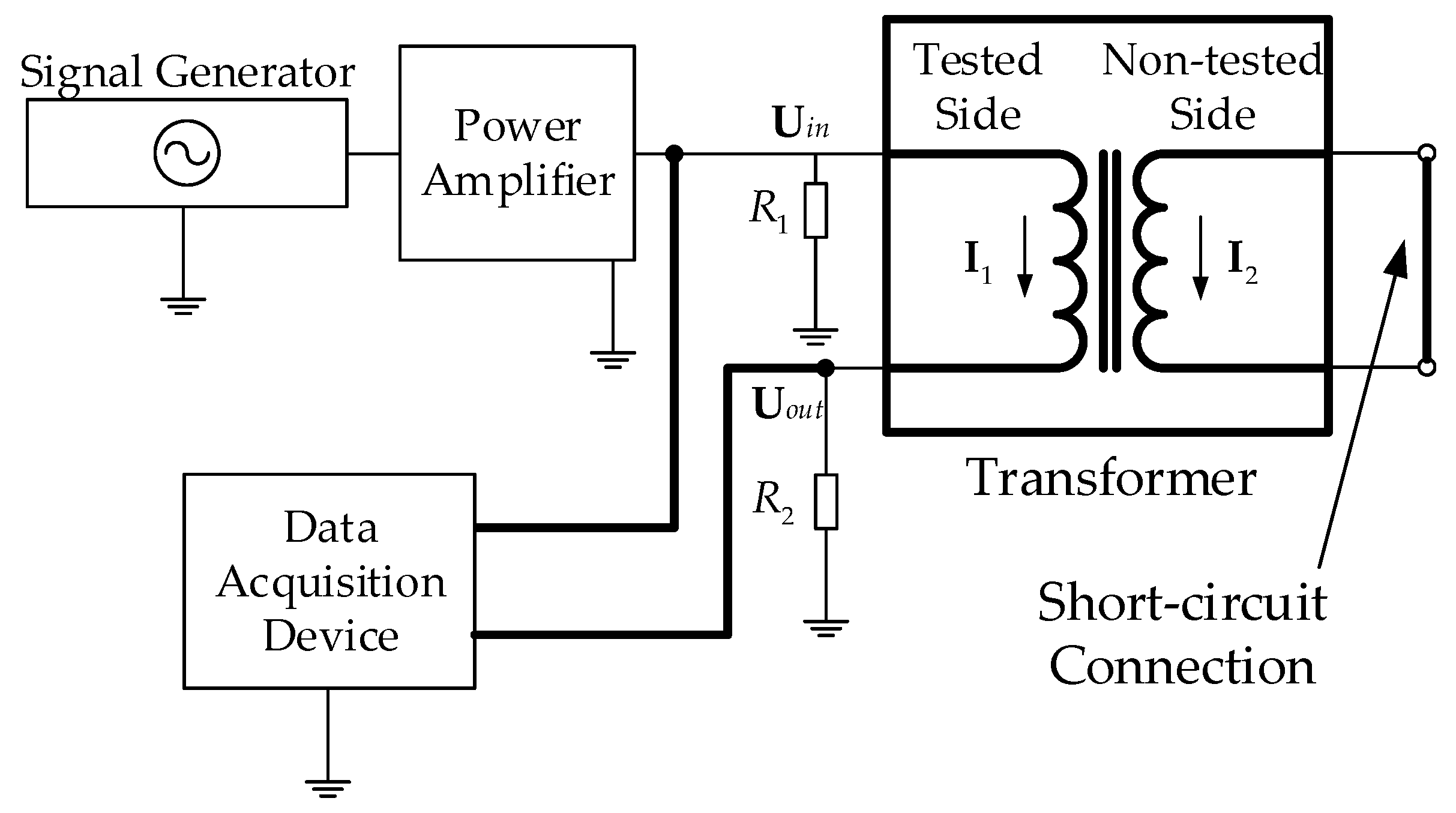
DLN is widely used to study the high-frequency characteristics of a two-winding transformer [3,13]. In this paper, based on the connection mode of the SFI measurements (see Figure 2), winding parameters were calculated using the FEM model and DLN, and a circuit model is proposed to simulate an SC fault of a transformer winding, as shown in Figure 8. In addition, the DLN sections from 1 to n represent the different winding discs in Figure 3, and R₃, connected between the (m + 1)th and nth nodes, stands for the resistance of the wire short-circuited the head and the end of the non-tested winding in Figure 2. As shown in Figure 8, in the SFI simulation of the HV winding, the numbers of tested nodes (1 to m) and non-tested nodes (m + 1 to n) are 49 and 52, respectively, which are equal to the number of HV and LV winding discs in Table 1. The specific circuit parameters in Figure 8 are defined as follows:

Cii, Gii	Ground capacitance and ground conductance of the ith (1 ≤ i ≤ n) winding disc;
Cij, Gij	Capacitance and conductance between the ith and jth (j ≠ i and 1 ≤ j ≤ n) discs;
Lii, Rii	Self-inductance and self-resistance of the ith disc;
Mij, Rij	Mutual inductance and mutual resistance between the disc i and j;
R0, L0	Resistance and inductance of the measurement line;
R1, R2	Sampling resistances of the signals, Uin and Uout;
R3	Resistance of the short-circuit wire.

The state vectors of the circuit model in Figure 8 consist of nodal voltages and inductor currents. Voltage and current equations can be written as follows:

$$-{\Gamma }^{T}I=C\dot{U}+GU,$$

(15)

and

$$\Gamma U=L\dot{I}+RI,$$

(16)

where L, R, C, and G represent the matrices of the inductance, resistance, capacitance, and conductance, respectively, and $\dot{U}$ and $\dot{I}$ (the dots on top of the symbols represent the derivatives of the state variables at the time) are, respectively, the time derivatives of the nodal voltage and inductor current matrices U and I. The matrix, Γ, consisting of 0, 1, and −1, is used to represent the connection mode between the current and voltage equations. Once the kth node is loaded with a voltage signal, U_k, the Equations (15) and (16) can be transformed as:

$$-{\left({\Gamma }^{\prime }\right)}^{T}I=C^{\prime }{\dot{U}}^{\prime }+G^{\prime }{U}^{\prime }+Q_C{\dot{U}}_k+Q_G{U}_k,$$

(17)

and

$$P{U}_k+{\Gamma }^{\prime }{U}^{\prime }=L\dot{I}+RI.$$

(18)

Here, C′ and G′ are obtained by removing the kth column and row from C and G, respectively. The matrices Q_C and Q_G contain the kth column of C and G without the kth row, respectively, and Γ′ is obtained by removing the kth column of Γ, while P contains the column with index k of matrix Γ.

When the signal U_k is a sinusoidal voltage, by using Laplace transformation, the Equations (17) and (18) are transformed into the frequency domain in the following way:

$$\left(\mathrm{j}\omega C^{\prime }+G^{\prime }\right)U^{\prime }+{\left({\Gamma }^{\prime }\right)}^{T}I=-\left(\mathrm{j}\omega Q_C+Q_G\right)U_k,$$

(19)

and

$${\Gamma }^{\prime }{U}^{\prime }-\left(\mathrm{j}\omega L+R\right)I=-P{U}_k.$$

(20)

where j is the imaginary unit and ω is the angular frequency. By rearranging the terms in (19) and (20), the state-space model of the circuit in Figure 8 can be obtained:

$$X=A^{-1}B{U}_k,$$

(21)

where

$$X=\left[\begin{array}{l}{U}^{\prime }\\ I\end{array}\right],A=\left[\begin{array}{cc}Y& {\left({\Gamma }^{\prime }\right)}^T\\ {\Gamma }^{\prime }& -Z\end{array}\right],\mathrm{and}B=\left[\begin{array}{l}-Y_u\\ -P\end{array}\right].$$

(22)

Here, Y, Y_u, and Z, respectively, stand for the matrices of the admittance and impedance in the circuit model, which are expressed as Y = jωC′ + G′, Y_u= jωQ_C+ Q_G, and Z = jωL + R.

Corresponding to the SFI measurement in Figure 2, in the SFI simulation, the external voltage source, U_in(jω), is connected to the 0th node in Figure 8. Based on (1) and (21), the simulated SFI signature, Z(jω), of a transformer winding can be numerically obtained from:

$$Z\left(\mathrm{j}\omega \right)=\left|\frac{U_0\left(\mathrm{j}\omega \right)-U_m\left(\mathrm{j}\omega \right)}{I_m\left(\mathrm{j}\omega \right)}\right|=\left|\frac{U_0\left(\mathrm{j}\omega \right)}{I_m\left(\mathrm{j}\omega \right)}-R_2\right|,$$

(23)

where U₀ and U_m represent the voltages of the 0th and mth nodes, respectively, and I_m is the current of the nth branch.

In conclusion, the general process of modelling SFI measurements, the parameter calculations, and the following correctness validation procedures used in this paper are illustrated in Figure 9.

5. Simulation and Experimental Verification

5.1. Simulation Verification

To verify the accuracy of the abovementioned modelling method, comparisons among the healthy winding SFI results obtained from the detailed model proposed in this paper, the model that did not consider FDCAPs, and the experimental measurements are plotted in Figure 10. All SFI experiments and simulations in this paper were carried out with a swept sinusoidal voltage of 30 V at a frequency range from 10 Hz to 1 MHz, and the number of measurement points was 99 from 10 Hz to 990 Hz, and 1000 from 1 kHz to 1 MHz, respectively. The abovementioned SFI experiments were conducted with the FLC F30PV power amplifier and TiePie HS-3 handy scope, which could be used to generate a swept sinusoidal voltage signal and acquire the excitation and response data. From the figures, it can be observed that the trend, resonance points, and amplitude of the simulation considering FDCAPs almost agree with the experimental SFI signatures when compared with the simulation results obtained from the model that did not consider these details. The differences between the simulation considering FDCAPs and the measurements mainly resulted from the computation error of the core permeabilities and the ignorance of the winding tap structure (see Figure 1) in the investigated transformer during the FEM modelling.

Furthermore, the widely employed indices, such as the integral of difference (ID), the absolute sum of the logarithmic error (ASLE), the spectrum deviation (SD), the stochastic spectrum deviation (SSD), and the sum squared ratio error (SSRE) [24], were used to numerically evaluate the similarity between the simulated and measured curves in Figure 10. The indices can be respectively obtained from:

$$ID={\displaystyle \int \left(y_i-x_i\right)}d{f}_i,$$

(24)

$$ASLE=\frac{{\displaystyle \sum _{i=1}^n\left|20{\log }_{10}{y}_i-20{\log }_{10}{x}_i\right|}}{n},$$

(25)

$$SD=\frac{1}{n}{\displaystyle \sum _{i=1}^n\sqrt{{\left(\frac{x_i-\left(x_i+y_i\right)/2}{\left(x_i+y_i\right)/2}\right)}^2+{\left(\frac{y_i-\left(x_i+y_i\right)/2}{\left(x_i+y_i\right)/2}\right)}^2}},$$

(26)

$$SSD=\frac{100}{n}{\displaystyle \sum _{i=1}^n\left|\frac{y_i-x_i}{x_i}\right|},$$

(27)

and

$$SSRE=\frac{{\displaystyle \sum _{i=1}^n{\left(\frac{y_i}{x_i}-1\right)}^2}}{n},$$

(28)

where x_i, y_i, and f_i represent, respectively, the ith element of the SFI vectors X = [x₁, x₂, …, x_n] and Y = [y₁, y₂, …, y_n] and the sampling frequencies, F = [f₁, f₂, …, f_n] (n is the total number of elements). The results of the indices between the simulations and the measurements are listed in

Table 3. Comparison of the simulation results and experimental measurements using numerical indices.

Location	Index Type	Detailed Model	Model without FDCAPs
HV winding	ID	0.3814 × 106	−3.4681 × 106
	ASLE	0.7959	1.6576
	SD	0.0281	0.0583
	SSD	3.9611	7.7081
	SSRE	0.0026	0.0119
LV winding	ID	−1.2844 × 106	−3.1689 × 106
	ASLE	3.6987	6.1752
	SD	0.1247	0.1826
	SSD	16.8017	20.1212
	SSRE	0.0409	0.0829

.

When the index values used in this paper are closer to 0, a higher similarity between the two sets of data can be obtained. Therefore, Table 3 indicates that the detailed model proposed in this paper is superior to that which did not consider FDCAPs. Based on the abovementioned comparisons, the accuracy of the model proposed in this paper is verified.

5.2. SC Faults

By shorting the circuit nodes or altering the winding shape of the FEM model, the model proposed in this paper can be employed to investigate SFI features of different forms of winding deformation, such as short circuits, axial displacement, radial displacement, and radial/hoop buckling, and so on. SC faults were used in the following case studies to verify the feasibility of using the model to research the SFI signatures of SC faults. The SC faults in this paper can be simulated by connecting a little resistance, R_sc, with the value of 1 × 10^–7 Ω between any two nodes in Figure 8. Figure 11 shows an example of an SC fault simulation, which illustrates SC fault settings in the circuit model.

5.2.1. Effects of SC Fault Levels

The impact of the SC fault level on the SFI curve was first investigated, and the level of the SC fault is defined as:

$$\Delta d=\frac{d_s}{d_t}\times 100\%,$$

(29)

where d_s is the number of shorted turns and d_t is the total turn number of the faulted winding. In this study, the SC faults were implemented in the top section of the HV winding, and their levels were, respectively, 2.04%, 4.08%, and 6.12%. The simulated SFI curves of the healthy and SC faults are shown in Figure 12.

As shown in Figure 12, when the SC faults occurred, the SFI curves of the HV winding presented an apparent right shift from 10 Hz to 700 kHz. Moreover, the impacts of the faults on the SFI curves above 20 kHz were more observable than those below 20 kHz. As the level of the SC fault increased, the abovementioned SFI trend was more obvious. Considering that the deviation of the SFI value of 50 Hz calculated in (4) is an important index for the detection of a winding fault, the impacts of SC faults on the SFI values of 50 Hz are listed in

Table 4. The simulated SFI deviations of 50 Hz between the faulted and healthy HV windings.

Condition	Z/Ω	ΔZ/%
Healthy	47.98	0
2.04%_SC	43.15	−10.07
4.08%_SC	42.81	−10.78
6.12%_SC	42.50	−11.42

.

From Table 4, it can be known that SC faults resulted in a reduction in the SFI value at 50 Hz, which manifested as a negative deviation value. Moreover, with the increase in the fault level, the changing trend of the SFI value at 50 Hz was more obvious, and the deviation, ΔZ, was smaller. Then, the same SC faults were implemented in the investigated transformer (see Figure 1), and the measurement results are plotted in Figure 13; in addition, the measured SFI values of 50 Hz and their corresponding deviations are listed in

Table 5. The deviations of the measured SFI values at 50 Hz between the faulted and healthy HV windings.

Condition	Z/Ω	ΔZ/%
Healthy	51.30	0
2.04%_SC	48.92	–4.64
4.08%_SC	45.18	–11.93
6.12%_SC	42.10	–17.93

.

As shown in Figure 13, the trends of the measured SFI curves with SC faults were the same as the simulated ones. Specifically, the SFI curves of the SC faults also presented an obvious right shift between 10 Hz and 700 kHz. With the increase in the SC fault level, the abovementioned change trend was also clearer; meanwhile, the measured SFI value at 50 Hz (see Table 5) decreased continuously. By comparison, the experimental results were the same as those of the simulation, which verifies that the proposed model can reflect the SFI signatures of the different levels of SC faults correctly.

5.2.2. Effects of SC Fault Positions

To research the capacity of the proposed model for simulating the actual SC faults on different positions of the transformer winding, the comparisons between the simulation and the measurements are shown in the following case study. The SC faults on the top, middle, and bottom sections of the HV winding in the investigated transformer were respectively implemented by connecting the taps of (1, 2), (17, 18), and (33, 34) in Figure 1b, which could be simulated by shorting the corresponding nodes in the circuit (see Figure 8), such as (2, 3), (18, 19), and (34, 35). The SFI results of the simulation and measurements are plotted in Figure 14 and Figure 15, respectively.

From Figure 14 and Figure 15, it can be observed that the change trends of the simulated and measured SFI curves are in satisfactory agreement when the SC fault occurs at different locations of the HV winding. Moreover, the SFI curves of all the SC faults present a right-shift trend, which is more obvious with the SC fault of the middle winding. Above 100 kHz, the resonance peak amplitudes of the SFI curves, reflecting SC faults of the middle and bottom windings, are greater than that of the healthy winding, which is different from that of the SC fault occurring in the top section of the winding.

Table 6. The simulated and measured SFI deviations of 50 Hz between the faulted and healthy HV windings.

Method	Condition	SFI Value/Ω	Deviation/%
Simulation	Healthy	47.98	0
	Top_SC	43.15	−10.07
	Middle_SC	40.67	−15.24
	Bottom_SC	40.88	−14.80
Measurement	Healthy	51.30	0
	Top_SC	48.92	−4.64
	Middle_SC	46.16	−10.02
	Bottom_SC	46.34	−9.67

lists the deviations of the simulated and measured SFI values at 50 Hz, where the variation of the SFI values caused by the SC fault in the middle winding is larger than the others. Meanwhile, when the SC fault occurred at different locations of the HV winding, the changing trend of the SFI deviation in the simulation was the same as that in the measurement, which indicates that introducing the proposed model to study the SFI features of SC faults at different winding locations is feasible.

5.2.3. Effects of SC Faults on the Non-Tested Winding

In this case, the impact of an SC fault of the non-tested winding on the SFI curve of the tested winding was investigated through measurement and simulation. The simulated and measured SFI results of the LV winding, before and after an SC fault of 6.12% implemented in the top section of the HV winding, are plotted in Figure 16 and Figure 17, respectively.

From Figure 16 and Figure 17, it can be seen that as the SC fault occurred in the HV winding, the SFI curve of the LV winding presented a left-shift trend at the high-frequency band, the ranges of which were above 900 kHz in the simulation and above 750 kHz in the measurement, respectively. However, the effect of the HV winding SC fault on the SFI curves of the LV winding was very slight and could be ignored. In

Table 7. The simulated and measured SFI deviations of the LV winding with the faulted and healthy HV windings.

Method	Condition	Z/Ω	ΔZ/%
Simulation	Healthy	1.02	0.00
	HV_SC	1.02	0.00
Measurement	Healthy	1.20	0.00
	HV_SC	1.20	0.00

, the deviation results, ΔZ, obtained from the simulation and the measurement were both 0.00, which indicates that the SC fault of the non-tested winding cannot influence the condition diagnosis of the tested winding. The abovementioned SFI features were wonderfully reflected in both the simulation and the measurements, which again verifies the correctness of the proposed model.

6. Conclusions

In this paper, a broadband model considering FDCAPs is proposed to study the impacts of SC faults on an SFI signature of a transformer winding. Furthermore, the accuracy of the proposed model was assessed by comparing its signature with those of other models, such as the simulation model without FDCAPs and the physical transformer model. The main conclusions are listed as follows:

• The simulation results from the model considering FDCAPs are in more agreement with experimental measurements than those of the model that did not consider FDCAPs, and the impacts of the same SC fault on the SFI curves obtained from the simulation considering FDCAPs and measurements were almost the same, which verifies that the proposed modelling approach can be effectively used to study the SFI features of SC faults.
• The SC fault could lead to a reduction in the SFI value at 50 Hz and a right shift of the SFI signature from 10 Hz to 700 kHz. As the level of the SC fault increased, the abovementioned trend was more significant.
• Unlike the SC fault in the top section of the winding, the SC faults occurring in the middle and bottom sections of the winding also resulted in high amplitudes of resonance peaks on SFI curves above 50 kHz. Meanwhile, the impact of the SC fault, occurring in the middle winding, on the SFI signature was more obvious.
• The SC fault of the non-tested winding could result in a slight left shift of the SFI curve within the tested winding at the high frequencies, but the change was too small to cause a misjudgment of the mechanical condition of the tested winding, which could be ignored in an onsite measurement.

In a word, the proposed model of a power transformer can be used to study the SFI features of SC faults accurately; meanwhile, the concluded SFI features of SC faults in this study contribute to the detection of an SC fault in a transformer winding. Moreover, it is expected that this paper may offer a new practicable idea for investigating the impacts of winding deformation on the SFI signature of a power transformer.

References

1. Hu, H.; Ma, X.; Shang, Y. A Novel Method for Transformer Fault Diagnosis Based on Refined Deep Residual Shrinkage Network. IET Electr. Power Appl. 2022, 16, 206–223. [Google Scholar] [CrossRef]
2. Karami, H.; Gharehpetian, G.B.; Norouzi, Y.; Akhavan-Hejazi, M. Simultaneous Radial Deformation and Partial Discharge Detection of High-Voltage Winding of Power Transformer. IET Electr. Power Appl. 2020, 14, 383–390. [Google Scholar] [CrossRef]
3. Ren, F.; Xiao, Y.; Zhan, C.; Liu, Y.; Yang, F.; Ji, S.; Zhu, L. Ladder Network Parameters Identification of an Isolated Winding by Combining the Intelligent Optimisation Algorithm and GNIA. IET Gener. Transm. Distrib. 2019, 13, 296–304. [Google Scholar] [CrossRef]
4. Meira, M.; Ruschetti, C.R.; Álvarez, R.E.; Verucchi, C.J. Power Transformers Monitoring Based on Electrical Measurements: State of the Art. IET Gener. Transm. Distrib. 2018, 12, 2805–2815. [Google Scholar] [CrossRef]
5. Zhou, L.; Jiang, J.; Li, W.; Wu, Z.; Gao, S.; Guo, L.; Liu, H. FRA Modelling for Diagnosing Axial Displacement of Windings in Traction Transformers. IET Electr. Power Appl. 2019, 13, 2121–2127. [Google Scholar] [CrossRef]
6. Moradzadeh, A.; Moayyed, H.; Mohammadi-Ivatloo, B.; Gharehpetian, G.B.; Aguiar, A.P. Turn-to-Turn Short Circuit Fault Localization in Transformer Winding via Image Processing and Deep Learning Method. IEEE Trans. Ind. Inform. 2022, 18, 4417–4426. [Google Scholar] [CrossRef]
7. Ren, F.; Ji, S.; Zhu, L.; Zhang, F.; Liu, Y. Generic Algorithm to Calculate Jacobian Matrix Used for Ladder Network Parameters Identification and Winding Fault Diagnosis. IET Gener. Transm. Distrib. 2019, 13, 3370–3377. [Google Scholar] [CrossRef]
8. Rajamani, R.; Rajappa, M.; Madanmohan, B. Sweep Frequency Response Analysis Based Diagnosis of Shorts within Transformer Windings. IET Gener. Transm. Distrib. 2017, 11, 4274–4281. [Google Scholar] [CrossRef]
9. Liu, Y.; Ji, S.; Yang, F.; Cui, Y.; Zhu, L.; Rao, Z.; Ke, C.; Yang, X. A Study of the Sweep Frequency Impedance Method and Its Application in the Detection of Internal Winding Short Circuit Faults in Power Transformers. IEEE Trans. Dielectr. Electr. Insul. 2015, 22, 2046–2056. [Google Scholar] [CrossRef]
10. Akhmetov, Y.; Nurmanova, V.; Bagheri, M.; Zollanvari, A.; Gharehpetian, G.B. A New Diagnostic Technique for Reliable Decision-Making on Transformer FRA Data in Interturn Short-Circuit Condition. IEEE Trans. Ind. Inform. 2021, 17, 3020–3031. [Google Scholar] [CrossRef]
11. Wang, S.; Wang, S.; Cui, Y.; Long, J.; Ren, F.; Ji, S.; Wang, S. An Experimental Study of the Sweep Frequency Impedance Method on the Winding Deformation of an Onsite Power Transformer. Energies 2020, 13, 3511. [Google Scholar] [CrossRef]
12. Zhao, X.; Yao, C.; Zhang, C.; Abu-Siada, A. Toward Reliable Interpretation of Power Transformer Sweep Frequency Impedance Signatures: Experimental Analysis. IEEE Electr. Insul. Mag. 2018, 34, 40–51. [Google Scholar] [CrossRef]
13. Zhao, X.; Yao, C.; Abu-Siada, A.; Liao, R. High Frequency Electric Circuit Modeling for Transformer Frequency Response Analysis Studies. Int. J. Electr. Power Energy Syst. 2019, 111, 351–368. [Google Scholar] [CrossRef]
14. Jahan, M.S.; Keypour, R.; Izadfar, H.R.; Keshavarzi, M.T. Detecting the Location and Severity of Transformer Winding Deformation by a Novel Adaptive Particle Swarm Optimization Algorithm. Int. Trans. Electr. Energy Syst. 2019, 29, e2666. [Google Scholar] [CrossRef]
15. Liang, G.; Gao, S.; Wang, Y.; Zang, Y.; Liu, X. Fractional Transmission Line Model of Oil-Immersed Transformer Windings Considering the Frequency-Dependent Parameters. IET Gener. Transm. Distrib. 2017, 11, 1154–1161. [Google Scholar] [CrossRef]
16. Shintemirov, A.; Tang, W.H.; Wu, Q.H. A Hybrid Winding Model of Disc-Type Power Transformers for Frequency Response Analysis. IEEE Trans. Power Deliv. 2009, 24, 730–739. [Google Scholar] [CrossRef]
17. Hashemnia, N.; Abu-Siada, A.; Islam, S. Improved Power Transformer Winding Fault Detection Using FRA Diagnostics–Part 1: Axial Displacement Simulation. IEEE Trans. Dielectr. Electr. Insul. 2015, 22, 556–563. [Google Scholar] [CrossRef]
18. Hashemnia, N.; Abu-Siada, A.; Islam, S. Detection of Power Transformer Bushing Faults and Oil Degradation Using Frequency Response Analysis. IEEE Trans. Dielectr. Electr. Insul. 2016, 23, 222–229. [Google Scholar] [CrossRef]
19. Abu-Siada, A.; Mosaad, M.I.; Kim, D.W.; El-Naggar, M.F. Estimating Power Transformer High Frequency Model Parameters Using Frequency Response Analysis. IEEE Trans. Power Deliv. 2020, 35, 1267–1277. [Google Scholar] [CrossRef]
20. Shamlou, A.; Feyzi, M.R.; Behjat, V. Interpretation of Frequency Response Analysis of Power Transformer Based on Evidence Theory. IET Gener. Transm. Distrib. 2019, 13, 3879–3887. [Google Scholar] [CrossRef]
21. Jiang, J.; Zhou, L.; Gao, S.; Li, W.; Wang, D. Frequency Response Features of Axial Displacement Winding Faults in Autotransformers With Split Windings. IEEE Trans. Power Deliv. 2018, 33, 1699–1706. [Google Scholar] [CrossRef]
22. Zhang, Z.W.; Tang, W.H.; Ji, T.Y.; Wu, Q.H. Finite-Element Modeling for Analysis of Radial Deformations Within Transformer Windings. IEEE Trans. Power Deliv. 2014, 29, 2297–2305. [Google Scholar] [CrossRef]
23. Solovei, V.D.; Dragoshanskii, Y.N. Magnetic Anisotropy Constants of a Fe-3.8% Si Single Crystal. Phys. Metals Metallogr. 2007, 103, 33–38. [Google Scholar] [CrossRef]
24. Bigdeli, M.; Azizian, D.; Gharehpetian, G.B. Detection of Probability of Occurrence, Type and Severity of Faults in Transformer Using Frequency Response Analysis Based Numerical Indices. Measurement 2021, 168, 108322. [Google Scholar] [CrossRef]
Figure 1. The investigated three-phase transformer: (a) front view; (b) oblique view of the internal structure.
Electronics 12 04068 g001
Figure 2. Connection diagram of SFI measurements.
Electronics 12 04068 g002
Figure 3. The FEM model of the investigated transformer.
Electronics 12 04068 g003
Figure 4. Computational methods for permeabilities of the FEM model.
Electronics 12 04068 g004
Figure 5. The meshes and the magnetic fluxes of the FEM model: (a) finite-element mesh; (b) magnetic fluxes at a frequency of 50 Hz; (c) magnetic fluxes at a frequency of 1 MHz.
Electronics 12 04068 g005
Figure 6. Some frequency-dependent inductances and resistances of the first disc on the phase C HV winding from 10 Hz to 1 MHz: (a) inductances; (b) resistances.
Electronics 12 04068 g006
Figure 7. Distribution of the electrical potential and FEM setting in the capacitance calculation.
Electronics 12 04068 g007
Figure 8. An equivalent circuit model of the SFI measurements based on a DLN.
Electronics 12 04068 g008
Figure 9. Flowchart for the calculation of parameters and SFI.
Electronics 12 04068 g009
Figure 10. Comparisons between the measured and simulated SFI curves of the healthy windings: (a) HV winding; (b) LV winding.
Electronics 12 04068 g010
Figure 11. The setting of an SC fault between the first and second nodes in the circuit model.
Electronics 12 04068 g011
Figure 12. Impacts of SC faults with different levels on the simulated SFI signature of the HV winding.
Electronics 12 04068 g012
Figure 13. Impacts of the SC faults with different levels on the measured SFI signature of the HV winding.
Electronics 12 04068 g013
Figure 14. The simulated SFI data of SC faults at different positions of the HV winding.
Electronics 12 04068 g014
Figure 15. The measured SFI data of SC faults at different positions of the HV winding.
Electronics 12 04068 g015
Figure 16. Impacts of HV wingding SC faults on the simulated SFI curve of the LV winding.
Electronics 12 04068 g016
Figure 17. Impacts of HV winding SC faults on the measured SFI curve of the LV winding.
Electronics 12 04068 g017