
FPQNet: Fully Pipelined and Quantized CNN for Ultra-Low Latency Image Classification on FPGAs Using OpenCAPI


Abstract
:1. Introduction
- We optimize the fully parallelized channel and fully pipelined layer structure with the HDMI timing standard to avoid extra data transfer and save hardware resources.
- We integrate the accelerator with a high-bandwidth OpenCAPI interface.
- We combine several proposed quantization and model compression methods to save hardware resources.
2. Background
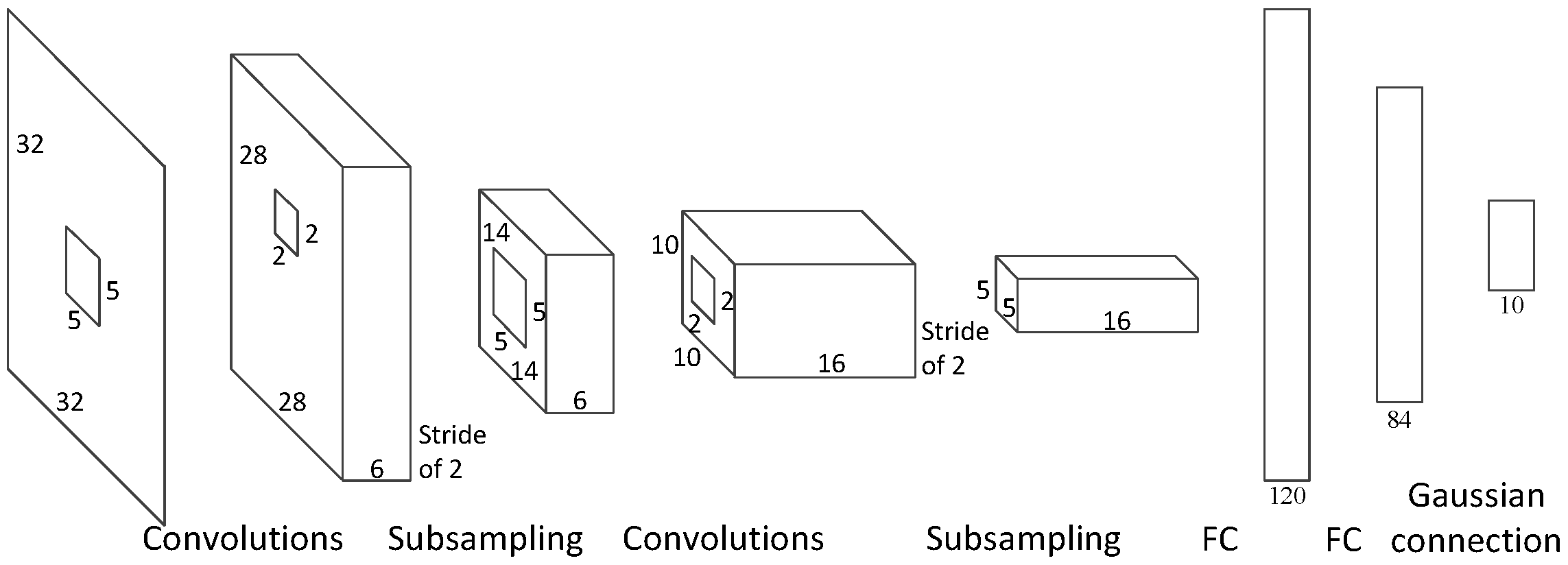
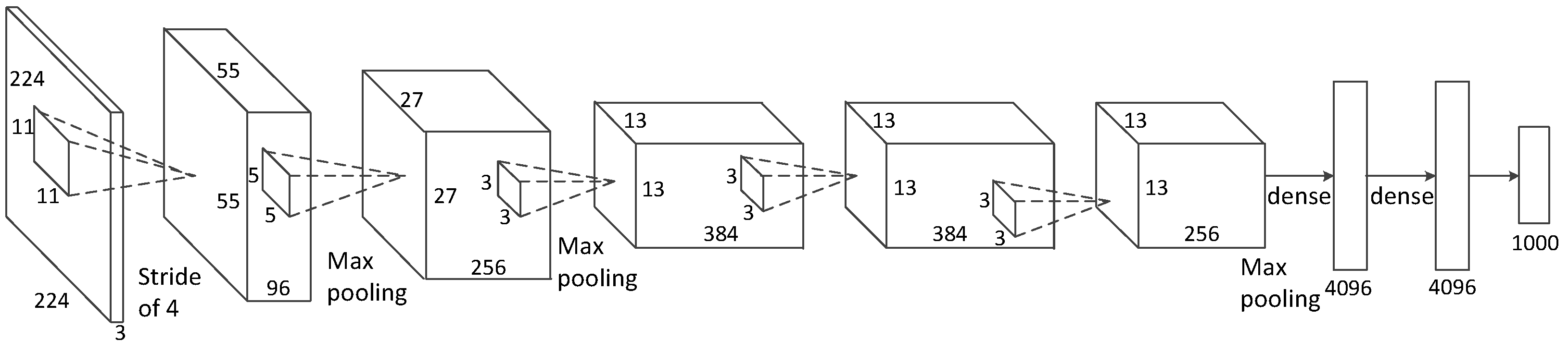
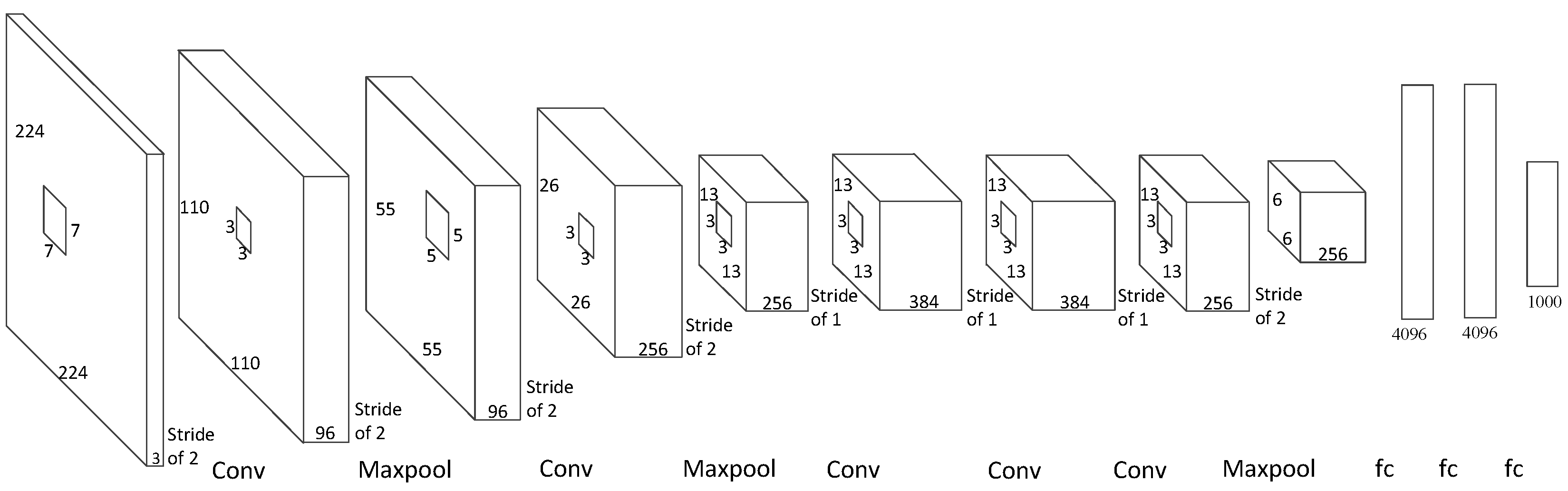
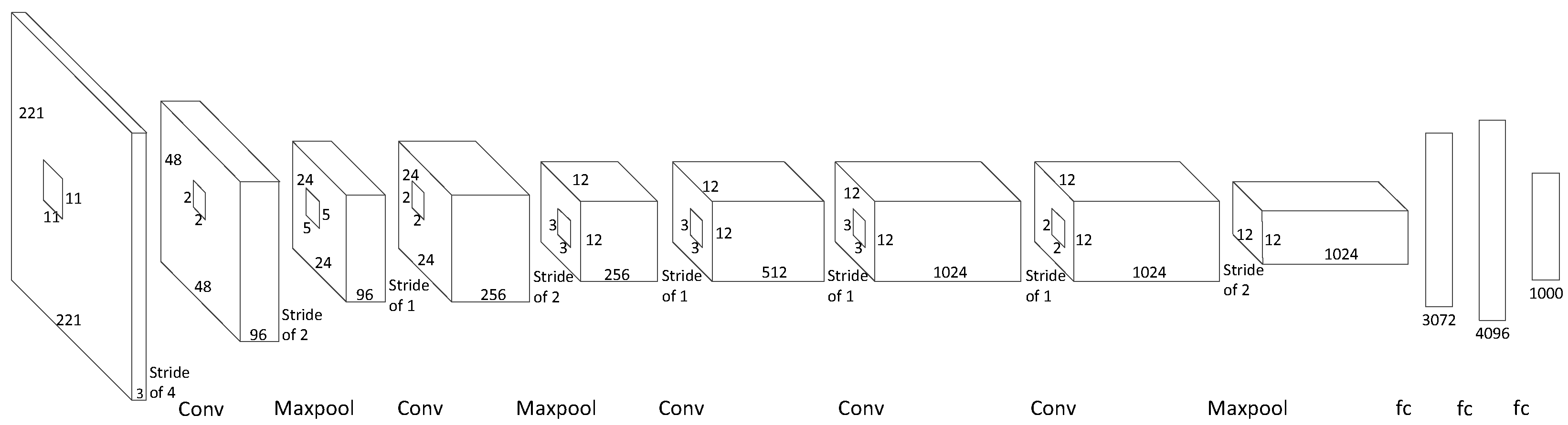
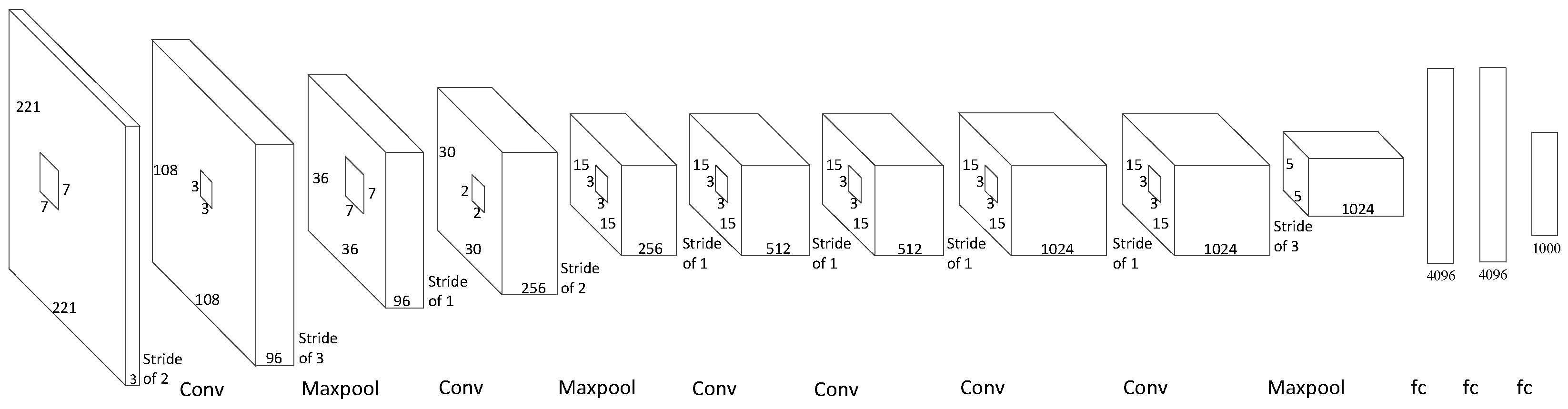
2.1. CNN Structures
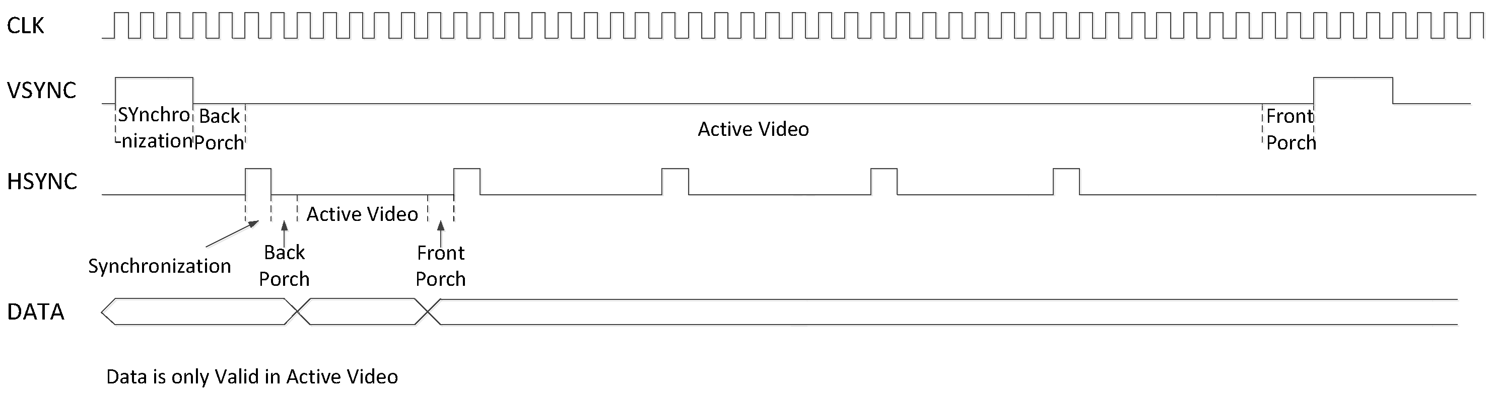
2.2. HDMI Timing Standard
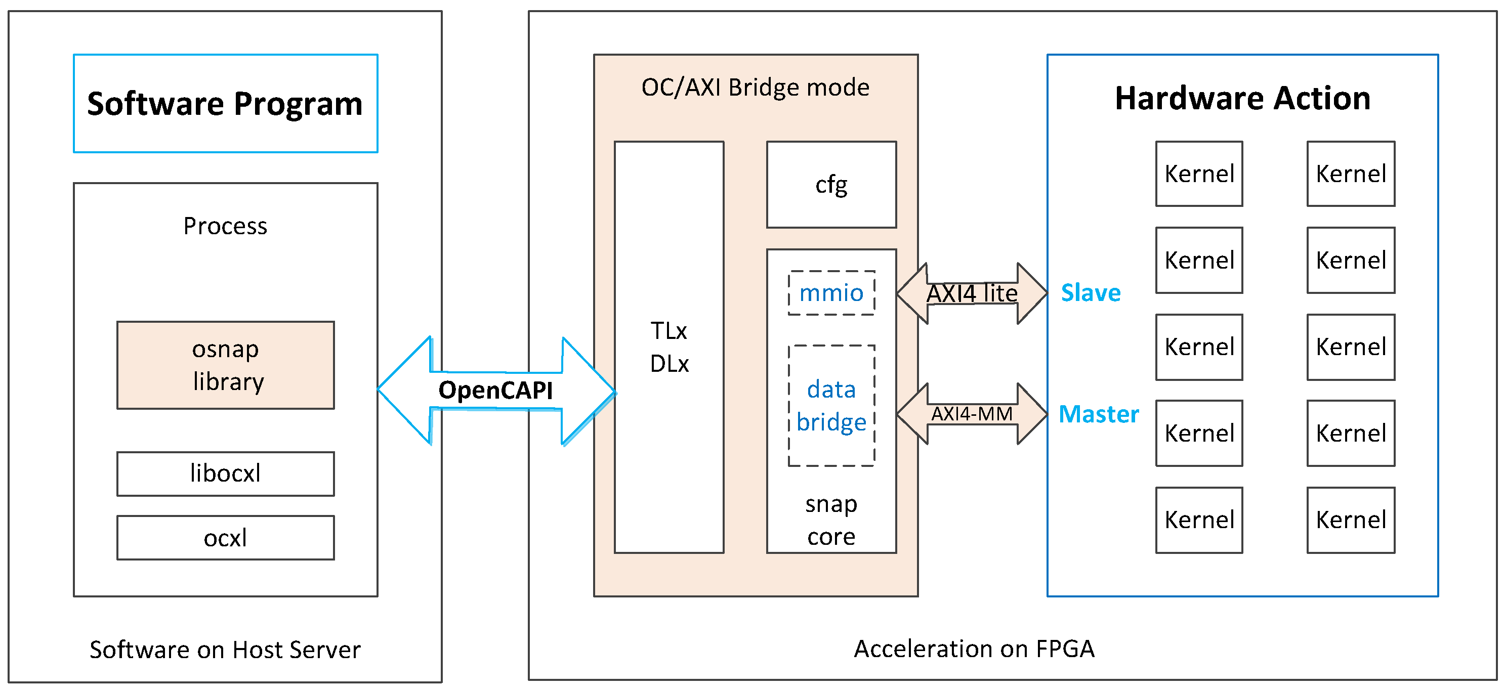
2.3. OpenCAPI Interface
3. Related Work
4. Algorithm Optimization
4.1. Improved Model
4.1.1. Reducing Input Size
4.1.2. Quantizing Parameters and Data
4.1.3. Improved Sigmoid Function
4.1.4. Output Layer Optimization
4.2. Result of Algorithm Optimization
5. Hardware Design
5.1. Overall Hardware Architecture on OpenCAPI
5.2. OpenCAPI Data Transfer Module
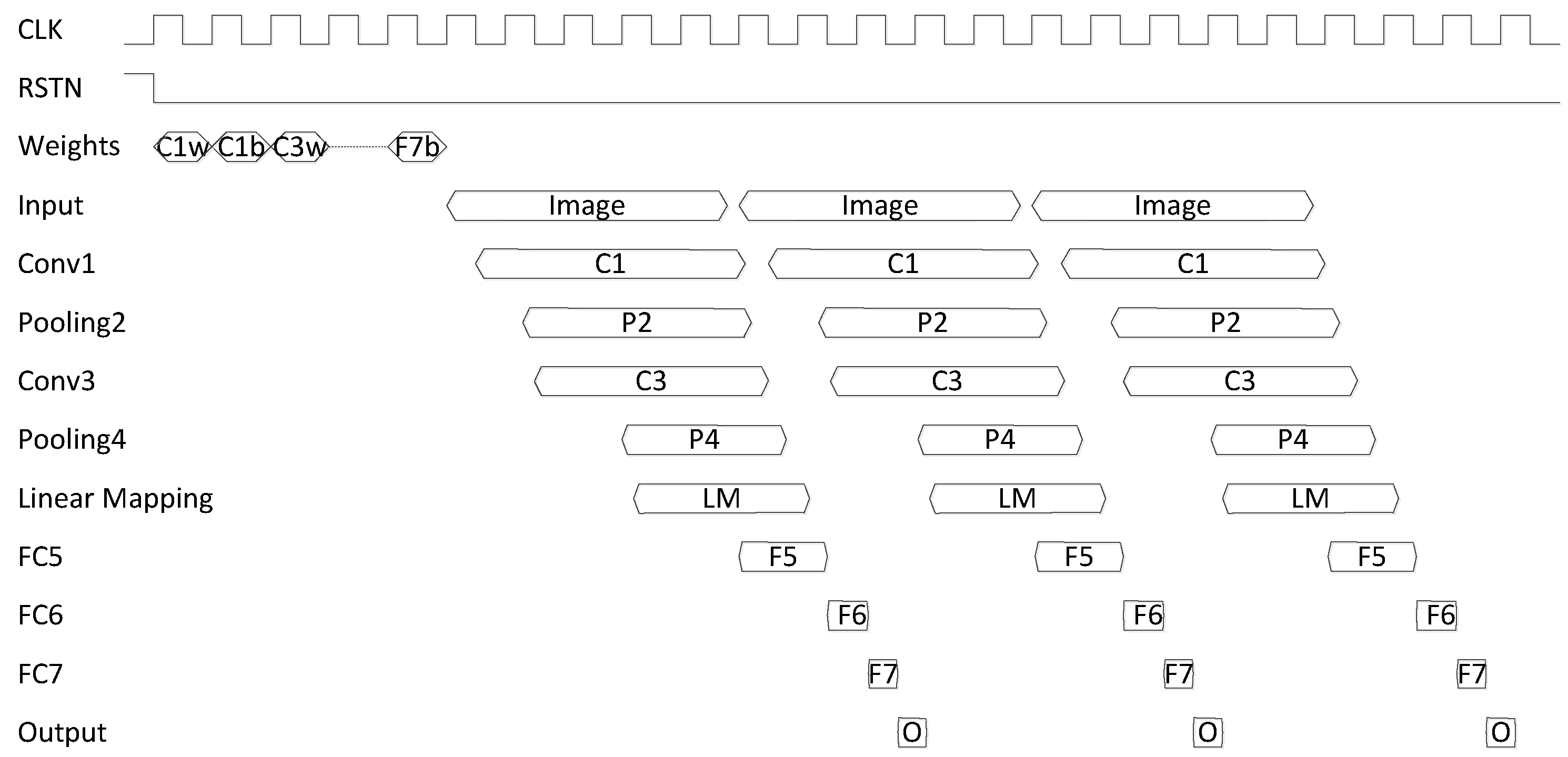
5.3. Layer-Pipeline Hardware Architecture
5.4. HDMI Timing Standard
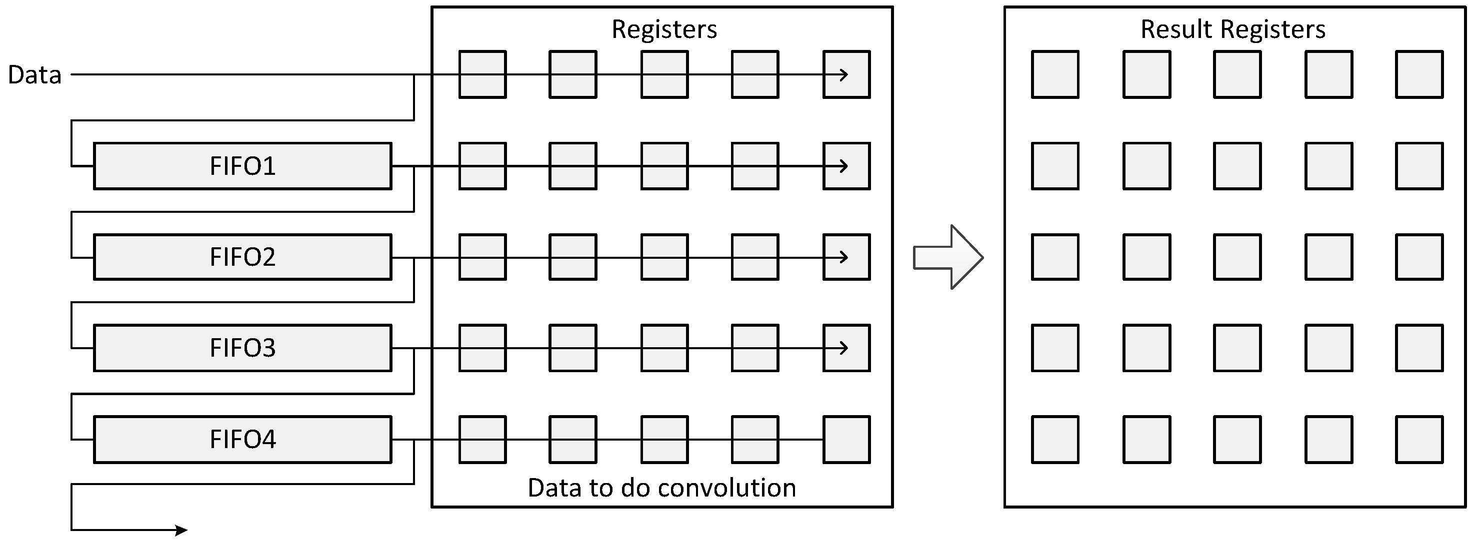
5.5. Convolution Layers
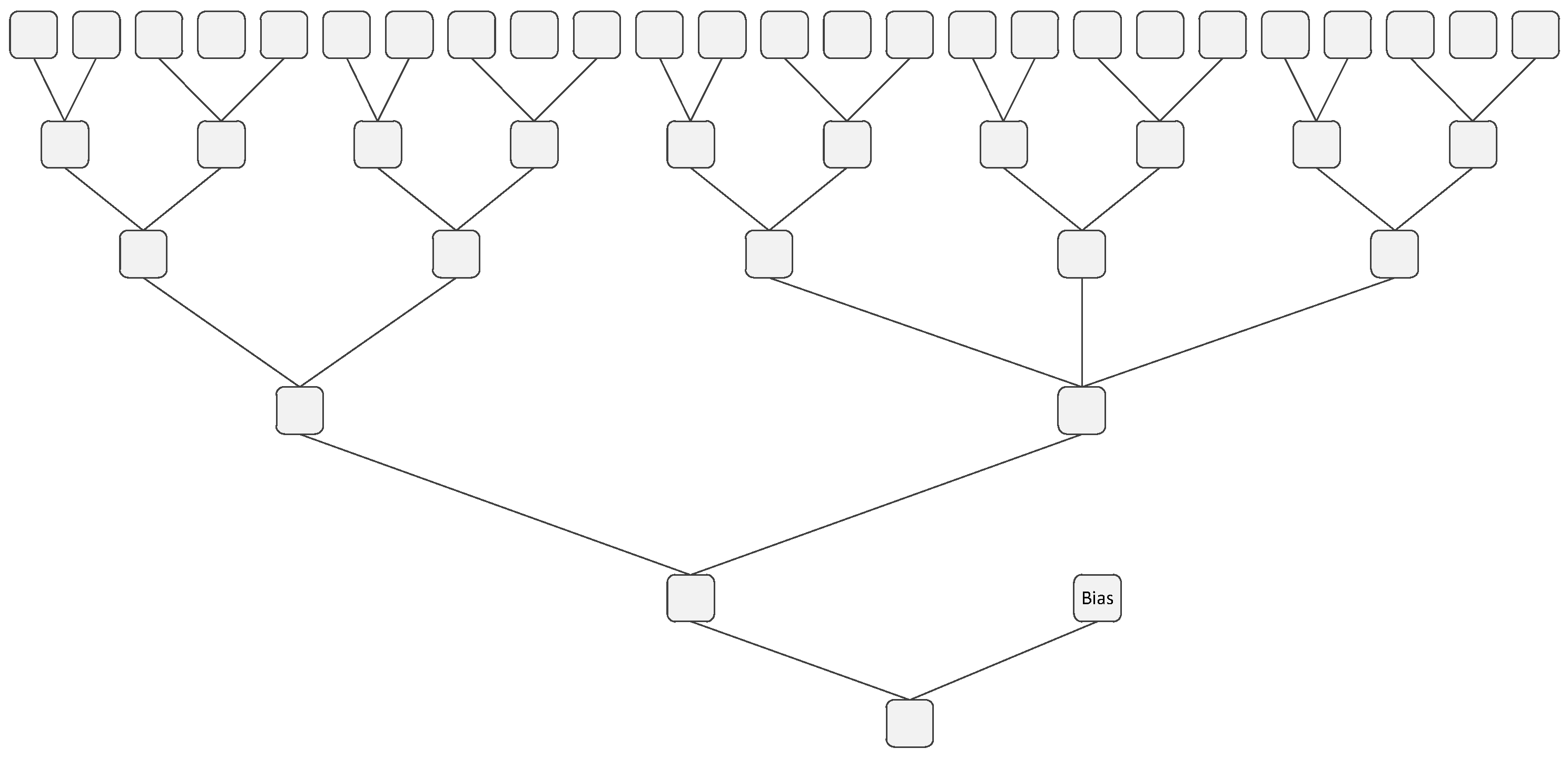
5.6. Pooling Layers
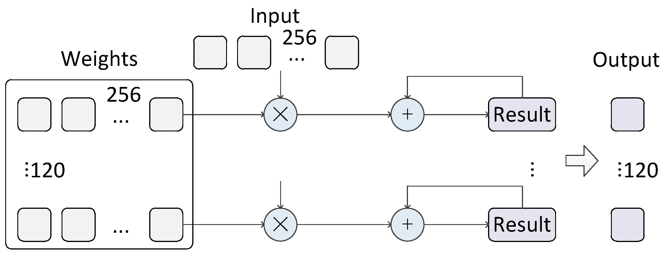
5.7. Fully Connected Layers and Output Layer
6. Experimental Results
6.1. Measurement Results
6.2. Comparison with Other Solutions
6.3. Comparison with FINN Solutions
6.4. Latency Analysis for Other CNNs
7. Conclusions
Author Contributions
Funding
Data Availability Statement
Conflicts of Interest
References
- Horng, S.J.; Supardi, J.; Zhou, W.L.; Lin, C.T.; Jiang, B. Recognizing Very Small Face Images Using Convolution Neural Networks. IEEE Trans. Intell. Transp. Syst. 2022, 23, 2103–2115. [Google Scholar] [CrossRef]
- Le, D.N.; Parvathy, V.S.; Gupta, D.; Khanna, A.; Rodrigues, J.; Shankar, K. IoT enabled depthwise separable convolution neural network with deep support vector machine for COVID-19 diagnosis and classification. Int. J. Mach. Learn. Cybern. 2021, 12, 3235–3248. [Google Scholar] [CrossRef]
- Sharifrazi, D.; Alizadehsani, R.; Roshanzamir, M.; Joloudari, J.H.; Shoeibi, A.; Jafari, M.; Hussain, S.; Sani, Z.A.; Hasanzadeh, F.; Khozeimeh, F.; et al. Fusion of convolution neural network, support vector machine and Sobel filter for accurate detection of COVID-19 patients using X-ray images. Biomed. Signal Process. Control 2021, 68, 102622. [Google Scholar] [CrossRef] [PubMed]
- Gao, S.H.; Cheng, M.M.; Zhao, K.; Zhang, X.Y.; Yang, M.H.; Torr, P. Res2Net: A New Multi-Scale Backbone Architecture. IEEE Trans. Pattern Anal. Mach. Intell. 2021, 43, 652–662. [Google Scholar] [CrossRef] [PubMed]
- Ye, T.; Zhang, X.; Zhang, Y.; Liu, J. Railway Traffic Object Detection Using Differential Feature Fusion Convolution Neural Network. IEEE Trans. Intell. Transp. Syst. 2021, 22, 1375–1387. [Google Scholar] [CrossRef]
- Jung, C.; Han, Q.H.; Zhou, K.L.; Xu, Y.Q. Multispectral Fusion of RGB and NIR Images Using Weighted Least Squares and Convolution Neural Networks. IEEE Open J. Signal Process. 2021, 2, 559–570. [Google Scholar] [CrossRef]
- Fukagai, T.; Maeda, K.; Tanabe, S.; Shirahata, K.; Tomita, Y.; Ike, A.; Nakagawa, A. Speed-up of object detection neural network with GPU. In Proceedings of the 25th IEEE International Conference on Image Processing (ICIP), Athens, Greece, 7–10 October 2018; pp. 301–305. [Google Scholar]
- Jung, W.; Dao, T.T.; Lee, J. DeepCuts: A Deep Learning Optimization Framework for Versatile GPUWorkloads. In Proceedings of the 42nd ACM SIGPLAN International Conference on Programming Language Design and Implementation (PLDI), Virtual, 20–25 June 2021; pp. 190–205. [Google Scholar]
- Ramakrishnan, R.; Dev, K.V.A.; Darshik, A.S.; Chinchwadkar, R.; Purnaprajna, M. Demystifying Compression Techniques in CNNs: CPU, GPU and FPGA cross-platform analysis. In Proceedings of the 34th International Conference on VLSI Design/20th International Conference on Embedded Systems (VLSID), Guwahati, India, 20–24 February 2021; pp. 240–245. [Google Scholar]
- Hsieh, M.H.; Liu, Y.T.; Chiueh, T.D. A Multiplier-Less Convolutional Neural Network Inference Accelerator for Intelligent Edge Devices. IEEE J. Emerg. Sel. Top. Circuits Syst. 2021, 11, 739–750. [Google Scholar] [CrossRef]
- Zhang, C.; Li, P.; Sun, G.; Guan, Y.; Xiao, B.; Cong, J. Optimizing FPGA-based accelerator design for deep convolutional neural networks. In Proceedings of the 2015 ACM/SIGDA International Symposium On Field-Programmable Gate Arrays, Monterey, CA, USA, 22–24 February 2015; pp. 161–170. [Google Scholar]
- Liu, L.Q.; Brown, S. Leveraging Fine-grained Structured Sparsity for CNN Inference on Systolic Array Architectures. In Proceedings of the 31st International Conference on Field-Programmable Logic and Applications (FPL), Dresden, Germany, 30 August–3 September 2021; pp. 301–305. [Google Scholar]
- Huang, W.J.; Wu, H.T.; Chen, Q.K.; Luo, C.H.; Zeng, S.H.; Li, T.R.; Huang, Y.H. FPGA-Based High-Throughput CNN Hardware Accelerator With High Computing Resource Utilization Ratio. IEEE Trans. Neural Netw. Learn. Syst. 2022, 33, 4069–4083. [Google Scholar] [CrossRef]
- Li, H.M.; Fan, X.T.; Jiao, L.; Cao, W.; Zhou, X.G.; Wang, L.L. A High Performance FPGA-based Accelerator for Large-Scale Convolutional Neural Networks. In Proceedings of the 26th International Conference on Field-Programmable Logic and Applications (FPL), Lausanne, Switzerland, 29 August–2 September 2016. [Google Scholar]
- Umuroglu, Y.; Fraser, N.J.; Gambardella, G.; Blott, M.; Leong, P.; Jahre, M.; Vissers, K. FINN: A Framework for Fast, Scalable Binarized Neural Network Inference. In Proceedings of the ACM/SIGDA International Symposium on Field-Programmable Gate Arrays, Monterey, CA, USA, 22–24 February 2017; pp. 65–74. [Google Scholar]
- Balasubramaniam, S.; Velmurugan, Y.; Jaganathan, D.; Dhanasekaran, S. A Modified LeNet CNN for Breast Cancer Diagnosis in Ultrasound Images. Diagnostics 2023, 13, 2746. [Google Scholar] [CrossRef]
- Yuan, Y.X.; Peng, L.N. Wireless Device Identification Based on Improved Convolutional Neural Network Model. In Proceedings of the 18th IEEE International Conference on Communication Technology (IEEE ICCT), Chongqing, China, 8–11 October 2018; pp. 683–687. [Google Scholar]
- Dubey, A. Agricultural plant disease detection and identification. Int. J. Electr. Eng. Technol. 2020, 11, 354–363. [Google Scholar]
- Lecun, Y.; Bottou, L.; Bengio, Y.; Haffner, P. Gradient-based learning applied to document recognition. Proc. IEEE 1998, 86, 2278–2324. [Google Scholar] [CrossRef]
- Krizhevsky, A.; Sutskever, I.; Hinton, G.E. ImageNet Classification with Deep Convolutional Neural Networks. Commun. ACM 2017, 60, 84–90. [Google Scholar] [CrossRef]
- Zeiler, M.D.; Fergus, R. Visualizing and Understanding Convolutional Networks. In Proceedings of the 13th European Conference on Computer Vision (ECCV), Zurich, Switzerland, 6–12 September 2014; pp. 818–833. [Google Scholar]
- Sermanet, P.; Eigen, D.; Zhang, X.; Mathieu, M.; Fergus, R.; LeCun, Y. Overfeat: Integrated recognition, localization and detection using convolutional networks. arXiv 2013, arXiv:1312.6229. [Google Scholar]
- Song, T.L.; Jeong, Y.R.; Yook, J.G. Modeling of Leaked Digital Video Signal and Information Recovery Rate as a Function of SNR. IEEE Trans. Electromagn. Compat. 2015, 57, 164–172. [Google Scholar] [CrossRef]
- Peltenburg, J.; Hadnagy, A.; Brobbel, M.; Morrow, R.; Al-Ars, A. Tens of gigabytes per second JSON-to-Arrow conversion with FPGA accelerators. In Proceedings of the 20th International Conference on Field-Programmable Technology (ICFPT), Auckland, New Zealand, 6–10 December 2021; pp. 194–202. [Google Scholar]
- Hoozemans, J.; Peltenburg, J.; Nonnemacher, F.; Hadnagy, A.; Al-Ars, Z.; Hofstee, H.P. FPGA Acceleration for Big Data Analytics: Challenges and Opportunities. IEEE Circuits Syst. Mag. 2021, 21, 30–47. [Google Scholar] [CrossRef]
- Lin, D.D.; Talathi, S.S.; Annapureddy, V.S. Fixed Point Quantization of Deep Convolutional Networks. In Proceedings of the 33rd International Conference on Machine Learning, New York, NY, USA, 19–24 June 2016. [Google Scholar]
- Zhu, B.; Hofstee, P.; Lee, J.; Alars, Z. Improving Gradient Paths for Binary Convolutional Neural Networks, BMVC 2022. Available online: https://bmvc2022.mpi-inf.mpg.de/0281.pdf (accessed on 18 August 2023).
- Liu, B.; Zou, D.Y.; Feng, L.; Feng, S.; Fu, P.; Li, J.B. An FPGA-Based CNN Accelerator Integrating Depthwise Separable Convolution. Electronics 2019, 8, 281. [Google Scholar] [CrossRef]
- Liu, B.; Zhou, Y.Z.; Feng, L.; Fu, H.S.; Fu, P. Hybrid CNN-SVM Inference Accelerator on FPGA Using HLS. Electronics 2022, 11, 2208. [Google Scholar] [CrossRef]
- Ma, Y.F.; Cao, Y.; Vrudhula, S.; Seo, J.S. Optimizing the Convolution Operation to Accelerate Deep Neural Networks on FPGA. IEEE Trans. Very Large Scale Integr. (Vlsi) Syst. 2018, 26, 1354–1367. [Google Scholar] [CrossRef]
- Cho, M.; Kim, Y. FPGA-Based Convolutional Neural Network Accelerator with Resource-Optimized Approximate Multiply-Accumulate Unit. Electronics 2021, 10, 2859. [Google Scholar] [CrossRef]
- Chen, J.Y.; Al-Ars, Z.; Hofstee, H.P. A Matrix-Multiply Unit for Posits in Reconfigurable Logic Leveraging (Open) CAPI. In Proceedings of the Conference on Next Generation Arithmetic (CoNGA), Singapore, 28 March 2018. [Google Scholar]
- Peltenburg, J.; van Leeuwen, L.T.J.; Hoozemans, J.; Fang, J.; Al-Ars, A.; Hofstee, H.P.; Soc, I.C. Battling the CPU Bottleneck in Apache Parquet to Arrow Conversion Using FPGA. In Proceedings of the 19th International Conference on Field-Programmable Technology (ICFPT), Maui, HI, USA, 9–11 December 2020; pp. 281–286. [Google Scholar]
- Zhu, B.Z.; Al-Ars, Z.; Pan, W. Towards Lossless Binary Convolutional Neural Networks Using Piecewise Approximation. In Proceedings of the 24th European Conference on Artificial Intelligence (ECAI), European Assoc Artificial Intelligence, Santiago de Compostela, Spain, 29 August–8 September 2020; pp. 1730–1737. [Google Scholar]
- Zhu, B.Z.; Al-Ars, Z.; Hofstee, H.P. NASB: Neural Architecture Search for Binary Convolutional Neural Networks. In Proceedings of the International Joint Conference on Neural Networks (IJCNN) Held as Part of the IEEE World Congress on Computational Intelligence (IEEE WCCI), Glasgow, UK, 19–24 July 2020. [Google Scholar]
- Baozhou, Z.; Hofstee, P.; Lee, J.; Al-Ars, Z. SoFAr: Shortcut-based fractal architectures for binary convolutional neural networks. arXiv 2020, arXiv:2009.05317. [Google Scholar]
- Zhou, S.; Wu, Y.; Ni, Z.; Zhou, X.; Wen, H.; Zou, Y. Dorefa-net: Training low bitwidth convolutional neural networks with low bitwidth gradients. arXiv 2016, arXiv:1606.06160. [Google Scholar]
- Otsu, N. Threshold Selection Method From Gray-Level Histograms. IEEE Trans. Syst. Man Cybern. 1979, 9, 62–66. [Google Scholar] [CrossRef]
- Han, J.; Moraga, C. The influence of the sigmoid function parameters on the speed of backpropagation learning. In International Workshop on Artificial Neural Networks; Springer: Berlin/Heidelberg, Germany, 1995; pp. 195–201. [Google Scholar]
- Liu, Z.C.; Luo, W.H.; Wu, B.Y.; Yang, X.; Liu, W.; Cheng, K.T. Bi-Real Net: Binarizing Deep Network Towards Real-Network Performance. Int. J. Comput. Vis. 2020, 128, 202–219. [Google Scholar] [CrossRef]
- Givaki, K.; Salami, B.; Hojabr, R.; Tayaranian, S.M.R.; Khonsari, A.; Rahmati, D.; Gorgin, S.; Cristal, A.; Unsal, O.S.; Soc, I.C. On the Resilience of Deep Learning for Reduced-voltage FPGAs. In Proceedings of the 28th Euromicro International Conference on Parallel, Distributed and Network-Based Processing (PDP), Vasteras, Sweden, 11–13 March 2020; pp. 110–117. [Google Scholar]
- Wang, H.; Wang, Y.T.; Zhou, Z.; Ji, X.; Gong, D.H.; Zhou, J.C.; Li, Z.F.; Liu, W. CosFace: Large Margin Cosine Loss for Deep Face Recognition. In Proceedings of the 31st IEEE/CVF Conference on Computer Vision and Pattern Recognition (CVPR), Salt Lake City, UT, USA, 18–23 June 2018; pp. 5265–5274. [Google Scholar]
- Qiao, S.J.; Ma, J. FPGA Implementation of Face Recognition System Based on Convolution Neural Network. In Proceedings of the Chinese Automation Congress (CAC), Xian, China, 30 November–2 December 2018; pp. 2430–2434. [Google Scholar]
- Molchanov, P.; Tyree, S.; Karras, T.; Aila, T.; Kautz, J. Pruning convolutional neural networks for resource efficient inference. arXiv 2016, arXiv:1611.06440. [Google Scholar]
- Zhang, L.; Bu, X.; Li, B. XNORCONV: CNNs accelerator implemented on FPGA using a hybrid CNNs structure and an inter-layer pipeline method. IET Image Process. 2020, 14, 105–113. [Google Scholar] [CrossRef]
- Laguduva, V.R.; Mahmud, S.; Aakur, S.N.; Karam, R.; Katkoori, S. Dissecting convolutional neural networks for efficient implementation on constrained platforms. In Proceedings of the 2020 33rd International Conference on VLSI Design and 2020 19th International Conference on Embedded Systems (VLSID), Bangalore, India, 4–8 January 2020; pp. 149–154. [Google Scholar]
- Li, Z.; Wang, L.; Guo, S.; Deng, Y.; Dou, Q.; Zhou, H.; Lu, W. Laius: An 8-bit fixed-point CNN hardware inference engine. In Proceedings of the 2017 IEEE International Symposium on Parallel and Distributed Processing with Applications and 2017 IEEE International Conference on Ubiquitous Computing and Communications (ISPA/IUCC), Guangzhou, China, 12–15 December 2017; pp. 143–150. [Google Scholar]
- Blott, M.; Preusser, T.B.; Fraser, N.J.; Gambardella, G.; O’Brien, K.; Umuroglu, Y.; Leeser, M.; Vissers, K. FINN-R: An End-to-End Deep-Learning Framework for Fast Exploration of Quantized Neural Networks. ACM Trans. Reconfig. Technol. Syst. 2018, 11, 1–23. [Google Scholar] [CrossRef]


| Resource | Available | Used | Utilization | Used | Utilization |
|---|---|---|---|---|---|
| One Net | Ten Nets | ||||
| LUTs | 1,303,680 | 53,292 | 4.09% | 1,061,205 | 81.40% |
| FFs | 2,607,360 | 94,470 | 3.62% | 1,131,786 | 43.41% |
| BRAMs | 2016 | 341 | 16.91% | 1465 | 72.67% |
| DSPs | 9024 | 2614 | 28.97% | 9024 | 100% |
| Reference | [45] | [46] | [47] | This Work | |
|---|---|---|---|---|---|
| One Net | Ten Nets | ||||
| FPGA platform | Zynq-7020 | PYNQ | Virtex7 485t | Alpha Data 9H7 | Alpha Data 9H7 |
| Layers | 6 | 7 | 7 | 7 | 7 |
| Frequency (MHz) | 150 | 650 | - | 250 | 250 |
| Data precision (bit) | 2 | - | 8 | 8 | 8 |
| Latency (µs) | 18.97 | 9100 | 490 | 9.32 | 9.32 |
| Accuracy | 98.4% | 97.06% | 98.16% | 98.8% | 98.8% |
| Throughput (GOPs) | - | 0.42 | 44.9 | 110.8 | 1108 |
| LUTs | 36,798 | - | 9071 | 53,292 | 1061 k |
| DSPs | 214 | - | 916 | 2614 | 9024 |
| BRAMs | 123 | - | 619 | 341 | 1465 |
| FINN | This Paper | |
|---|---|---|
| Model | LeNet-5 | LeNet-5 |
| Weight precision (bit) | 8 | 8 |
| Activation precision (bit) | 8 | 8 |
| FPGA platform | Alveo U200 | Alpha Data 9H7 |
| Frequency (MHz) | 250 | 250 |
| Accuracy | 98.8% | 98.8% |
| Throughput | 17,193.95 fps | 110.8 GOPs |
| Latency (µs) | 230.38 | 9.32 |
| BRAM utilization | 32 | 341 |
| LUT utilization | 66,931 | 53,292 |
| DSP utilization | 0 | 2614 |
| Model | LeNet-5 | LeNet-5 | LeNet-5 | LeNet-5 |
|---|---|---|---|---|
| Weight precision (bit) | 8 | 8 | 2 | 2 |
| Activation precision (bit) | 2 | 1 | 2 | 1 |
| FPGA platform | Alveo U200 | Alveo U200 | Alveo U200 | Alveo U200 |
| Frequency (MHz) | 250 | 250 | 250 | 250 |
| Accuracy | 98.6% | 98.2% | 98.6% | 97.5% |
| Throughput (fps) | 17,193.95 | 17,193.95 | 17,193.95 | 17,193.95 |
| Latency (µs) | 231.02 | 231.02 | 231.02 | 231.02 |
| BRAM utilization | 32 | 32 | 10 | 10 |
| LUT utilization | 5267 | 4754 | 3145 | 2811 |
| Layer | Cycle |
|---|---|
| ConvolutionInputGenerator_0 | 14,540 |
| MatrixVectorActivation_0 | 3456 |
| StreamingMaxPool_Batch_0 | 720 |
| ConvolutionInputGenerator_1 | 9960 |
| MatrixVectorActivation_1 | 10,240 |
| StreamingMaxPool_Batch_1 | 80 |
| MatrixVectorActivation_2 | 7680 |
| MatrixVectorActivation_3 | 10,080 |
| MatrixVectorActivation_4 | 840 |
| Latency (µs) | Conv1 | Pool2 | Conv3 | Pool4 | Conv5 | Conv6 | Conv7 |
|---|---|---|---|---|---|---|---|
| AlexNet | 9.86 | 0.66 | 0.54 | 0.32 | 0.16 | 0.16 | - |
| ZFNet | 6.27 | 1.32 | 1.10 | 0.31 | 0.16 | 0.16 | - |
| OverFeat-Fast | 10.16 | 3.84 | 0.48 | 0.10 | 0.14 | 0.14 | - |
| OverFeat-Accurate | 6.19 | 1.30 | 1.01 | 0.36 | 0.18 | 0.18 | 0.18 |
| Latency (µs) | Conv8 | Pool9 | FC1 | FC2 | FC3 | Output | Total |
| AlexNet | 0.16 | 0.16 | 0.07 | 36.86 | 16.38 | 4.00 | 69.27 |
| ZFNet | 0.16 | 0.16 | 0.07 | 36.86 | 16.38 | 4.00 | 66.95 |
| OverFeat-Fast | 0.14 | 0.10 | 0.04 | 147.46 | 16.38 | 4.00 | 182.98 |
| OverFeat-Accurate | 0.18 | 0.18 | 0.06 | 102.40 | 16.38 | 4.00 | 132.6 |
Disclaimer/Publisher’s Note: The statements, opinions and data contained in all publications are solely those of the individual author(s) and contributor(s) and not of MDPI and/or the editor(s). MDPI and/or the editor(s) disclaim responsibility for any injury to people or property resulting from any ideas, methods, instructions or products referred to in the content. |
© 2023 by the authors. Licensee MDPI, Basel, Switzerland. This article is an open access article distributed under the terms and conditions of the Creative Commons Attribution (CC BY) license (https://creativecommons.org/licenses/by/4.0/).
Share and Cite
Ji, M.; Al-Ars, Z.; Hofstee, P.; Chang, Y.; Zhang, B. FPQNet: Fully Pipelined and Quantized CNN for Ultra-Low Latency Image Classification on FPGAs Using OpenCAPI. Electronics 2023, 12, 4085. https://doi.org/10.3390/electronics12194085
Ji M, Al-Ars Z, Hofstee P, Chang Y, Zhang B. FPQNet: Fully Pipelined and Quantized CNN for Ultra-Low Latency Image Classification on FPGAs Using OpenCAPI. Electronics. 2023; 12(19):4085. https://doi.org/10.3390/electronics12194085
Chicago/Turabian StyleJi, Mengfei, Zaid Al-Ars, Peter Hofstee, Yuchun Chang, and Baolin Zhang. 2023. "FPQNet: Fully Pipelined and Quantized CNN for Ultra-Low Latency Image Classification on FPGAs Using OpenCAPI" Electronics 12, no. 19: 4085. https://doi.org/10.3390/electronics12194085
APA StyleJi, M., Al-Ars, Z., Hofstee, P., Chang, Y., & Zhang, B. (2023). FPQNet: Fully Pipelined and Quantized CNN for Ultra-Low Latency Image Classification on FPGAs Using OpenCAPI. Electronics, 12(19), 4085. https://doi.org/10.3390/electronics12194085