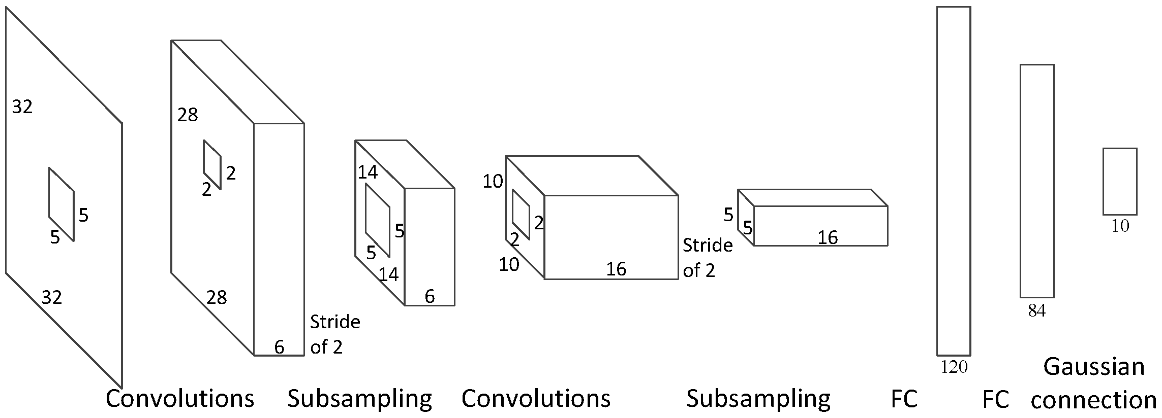
In this section, we show our hardware experimental results for our FPQNet implementation. We also compare our results with other solutions and discuss the advantages and disadvantages of our design. Furthermore, we analyze the latency of other popular convolutional neural networks. The code for this work can only be used for this specific LeNet-5 network. However, the same design approach can be used to implement the proposed hardware techniques for other networks.
6.1. Measurement Results
The experimental setup used in this paper to perform the measurements consists of an Inspur FP5290G2 system with a dual-socket POWER9 Lagrange 22-core CPU and OpenCAPI interface to an Aphadata ADM-PCIE-9H7 FPGA board, with a Xilinx XCVU37P chip. Our design is implemented via Verilog hardware design language rather than HLS tools. Our network design runs at a 250 MHz clock frequency. We also use the MNIST dataset for inference measurements.
Measurements show that our design can achieve an ultra-low latency inference time for each MNIST image that is as low as 9.32 µs. Due to the predictable operation of the FPGA designs, all MNIST images run at that exact timing. This indicates that it is possible to use such FPGA ML designs to perform inference in applications that require real-time inference capabilities as well as predictable timing.
The latency to transfer the parameters from CPU to FPGA is 222 µs. However, we only need to transfer the weights once and then can infer multiple images continuously. Therefore, this transfer of parameters is not part of the latency-critical path. When transferring the images and transferring the results back to the CPU for multiple kernels, the high bandwidth of OpenCAPI can avoid a bottleneck.
The hardware utilization values of the FPGA resources for the full designs of one network and ten parallel networks are listed in
Table 1. These numbers include the full hardware, including the one or ten convolutional neural network designs, as well as the OpenCAPI interfacing infrastructure. The table shows that the utilization values of the DSPs, BRAMs, and LUTs for one network are 28.97%, 16.91%, and 4.09%. The utilization values of the DSPs, BRAMs, and LUTs for ten networks are 100%, 72.67%, and 81.4%, respectively. One network only uses about one-tenth of the resources on FPGA and multiple networks make almost full use of the resources on FPGA.
As discussed earlier in the paper, the design can achieve an accuracy of 98.8%.
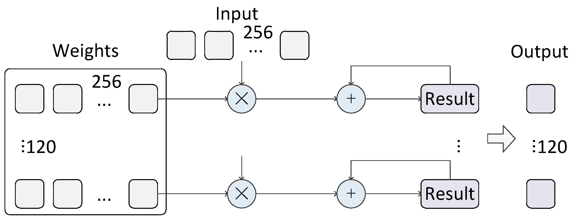
To calculate the throughput, we need to calculate the number of floating-point operations (FLOPs) used by the network first. Now, we calculate the FLOPs of one LeNet-5 convolutional neural network. For convolutional layers, pooling layers, and fully connected layers, we follow the method in [
44]. The FLOP numbers for convolutional layers, pooling layers, and fully connected layers are 940,416, 4480, and 83,280, respectively. For the optimized Sigmoid function, each input pixel only needs to undergo one operation, making the total FLOPs for all the Sigmoid functions 4684. For the max operation in the output layer, each input pixel needs to undergo one operation; therefore, the FLOPs of this operation is 10. In total, the number of FLOPs of all operations in one network is 1,032,870, which gives a throughput of 1,032,870/9.32 µs = 110.8 GOPs. Ten neural networks working together make the overall throughput 1108 GOPs. This is the highest throughput reported for accelerating LeNet on FPGAs.
From the Vivado report, the power consumption of one LeNet implementation is 420 W. The static power consumption is 37.0 W, which is 9% of the total power consumption and the dynamic power consumption is 383 W, which is 91% of the total power consumption.
6.2. Comparison with Other Solutions
In
Table 2, we compare our FPQNet implementation with former implementations of the LeNet network on FPGAs. The accuracy results are all based on inference measurement on the MNIST dataset.
Compared to [
45], the latency of 9.32 µs in our implementation is about half of the latency of 18.97 µs in the cited paper. Considering that the frequency of the cited paper is lower than ours, we run a simulation with a reduced frequency equal to that in [
45]. This increases our latency to 15.5 µs, which is 18.1% lower than the latency in [
45]. Another difference between the two implementations is that the cited paper uses the original dataset image size while we optimize the image by reducing its size. On the other hand, our design is targeted toward video processing; therefore, our design includes the horizontal/vertical back/front porch signals for the images, which is not included in [
45]. Due to these differences, it is not possible to provide a direct fair comparison between the latency of the two designs. In addition, our accuracy is 0.4% higher than the accuracy in [
45]. However, our implementation uses 1.4 times more LUTs, 12.2 times more DSPs, and 2.8 times more BRAMs. Compared to [
46], our latency is about 1000 times lower and our throughput is 264 times higher, despite the fact that they use higher frequencies. At the same time, our accuracy is 1.74% higher than the accuracy in [
46]. Reference [
47] shows a 53 times higher latency and a 2.5 times lower throughput than our implementation. At the same time, our implementation uses 5.9 times more LUTs and 2.9 times more DSPs but about half of the BRAMs compared to [
47].
The table shows that our FPQNet design is able to achieve the lowest latency of all available published solutions, scoring less than half of the lowest latency of any of the alternatives. With 10 networks working together, the overall throughput achieved is almost 25 times higher than other reported designs. However, this comes at the expense of high resource utilization. The resources are used to enable the parallelization needed to achieve lower latency and higher throughput. Still, for modern-day FPGAs, the continued increase in available resources makes such a trade-off viable. In terms of accuracy, with our optimized methods, our design has the highest accuracy of 98.8% among these designs.
6.3. Comparison with FINN Solutions
We compare the results in this paper with the results of the same CNN model implemented by FINN [
15,
48]. We train the same LeNet-5 model with Brevitas. We use the batch size of 256, the learning rate of 0.001, the epoch number of 40, and an Adam optimizer to train the model. The pooling layer is changed from the average pooling layer to the max-pooling layer because we are not able to obtain a good accuracy result using the average pooling layer. After training, we use FINN 0.8.1 to implement the model as well as Alveo U200 FPGA to implement the model. The comparison of the results of the model implemented by FINN and the manually implemented model in this paper is shown in
Table 3.
The table shows that—with the same data precision as the LeNet-5 model implemented manually in this paper, which is 8 bits for the weights and 8 bits for the activations—the FINN implementation shows the same accuracy result. The lowest latency that FINN models can achieve is 230.38 µs, which is 24.7× higher compared to the latency of 9.32 µs in our implementation. The LUT utilization of this FINN model is 66,931, which is 25.6% higher than our implementation. The BRAM utilization of the FINN implementation is 32, which is 9.4% of our implementation, and our implementation utilizes 2614 DSPs, whereas the FINN implementation does not employ DSPs.
We also implement the LeNet-5 models with other bit widths in FINN. The results of the FINN implementations of models with other bit widths of data precision are also shown in
Table 4. The lowest latency and the highest throughput that the FINN implementations can achieve are similar. When increasing the bit width of the data precision, the accuracy of the models increases, while the resource utilization of the implementation also increases.
Here, we further explore the reason for the large gap in latency between the results of FINN and the results of our implementation. We look into the latency results of each layer of the CNN model of FINN. The latency of each layer is shown in
Table 5. The latency is presented by the number of clock cycles used. As shown in the table, the bottleneck of the design is the first ConvolutionInputGenerator layer, which takes 14,540 clock cycles. The main operation of FINN is based on matrix–vector multiplications. FINN maps each layer of a CNN to a dedicated processing engine named the matrix–vector–threshold unit (MVTU). Every convolutional layer is converted into a sliding window unit (SWU), which generates the image matrix from incoming feature maps, and an MVTU. The ConvolutionInputGenerator in
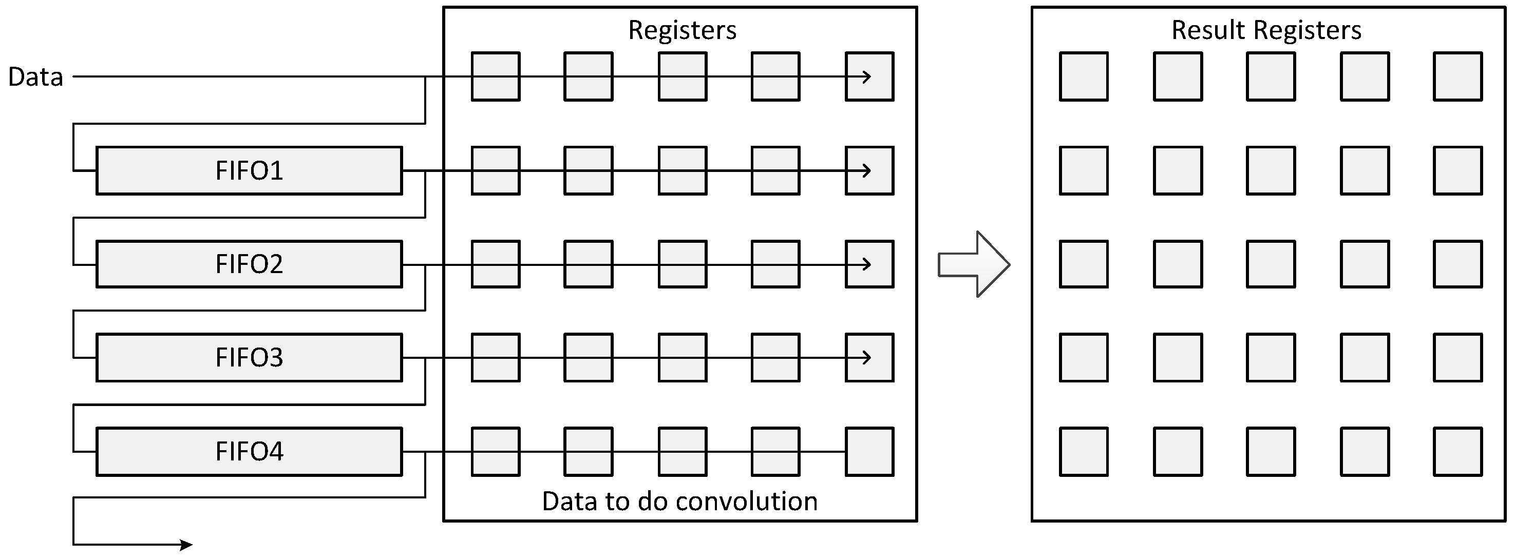
Table 5 is the SWU. The time that FINN needs to generate the input features into the matrix, which is needed for the next step, is long, because it needs to copy data multiple times, and it cannot be parallel when the input only has one channel. However, our design in this paper directly uses FIFOs to store data for the convolution operation, such that data can stream in one by one, and the convolution operation can start and continue to work as long as the kernel size line data are streamed in. In this way, our design does not have the same bottleneck as FINN.
However, FINN is an automated design framework, which requires less effort to implement a neural network. As an example, for the LeNet-5 designs in this paper, it took us two months to implement the network manually, as compared with two days to implement in FINN.
In conclusion, the results show that FINN can implement a model efficiently and flexibly, and FINN can achieve a trade-off between latency and resource utilization. However, FINN does not focus on implementing extremely low latency implementations. In situations that have strict latency requirements but have sufficient hardware resources and enough human costs, the implementation strategy represented in this paper works better than the FINN implementations.
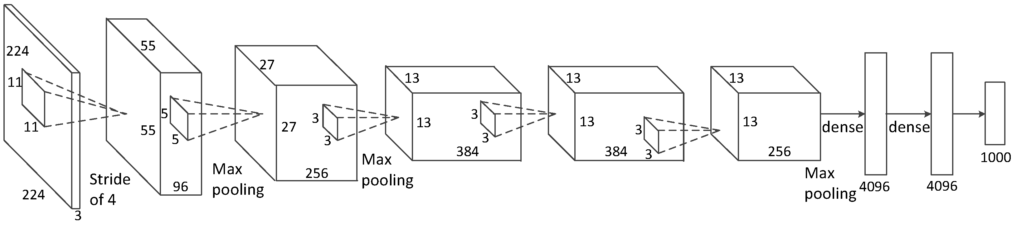
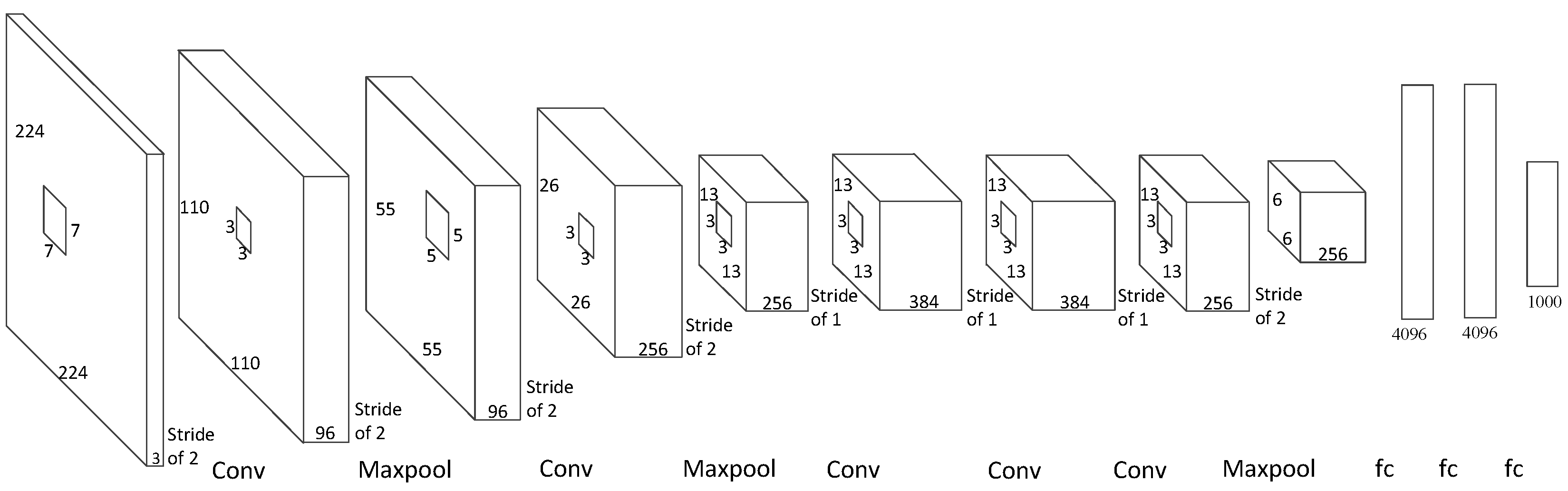
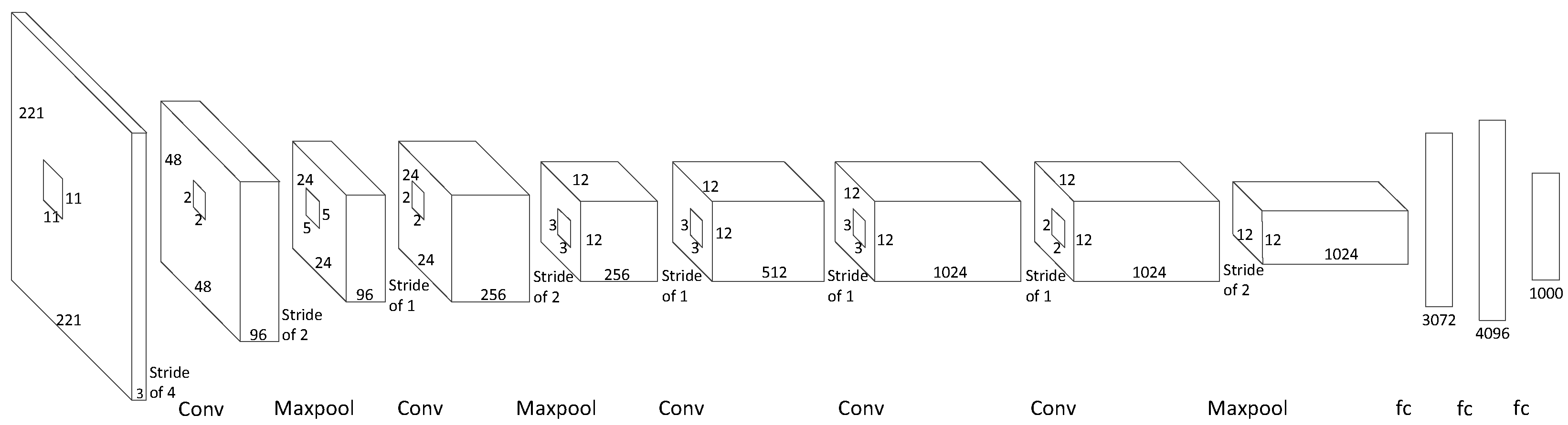
6.4. Latency Analysis for Other CNNs
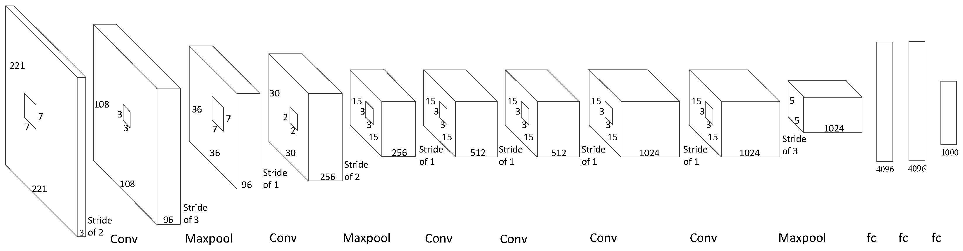
The architecture we show in this paper can be used in many other convolutional neural networks, such as AlexNet, ZFNet, and OverFeat. In this section, we estimate the latency we expect to achieve by implementing our architecture to several other networks. Due to the labor-intensive nature of the hardware implementation, we focus on estimating the impact of our architecture rather than on a detailed hardware implementation. As shown in
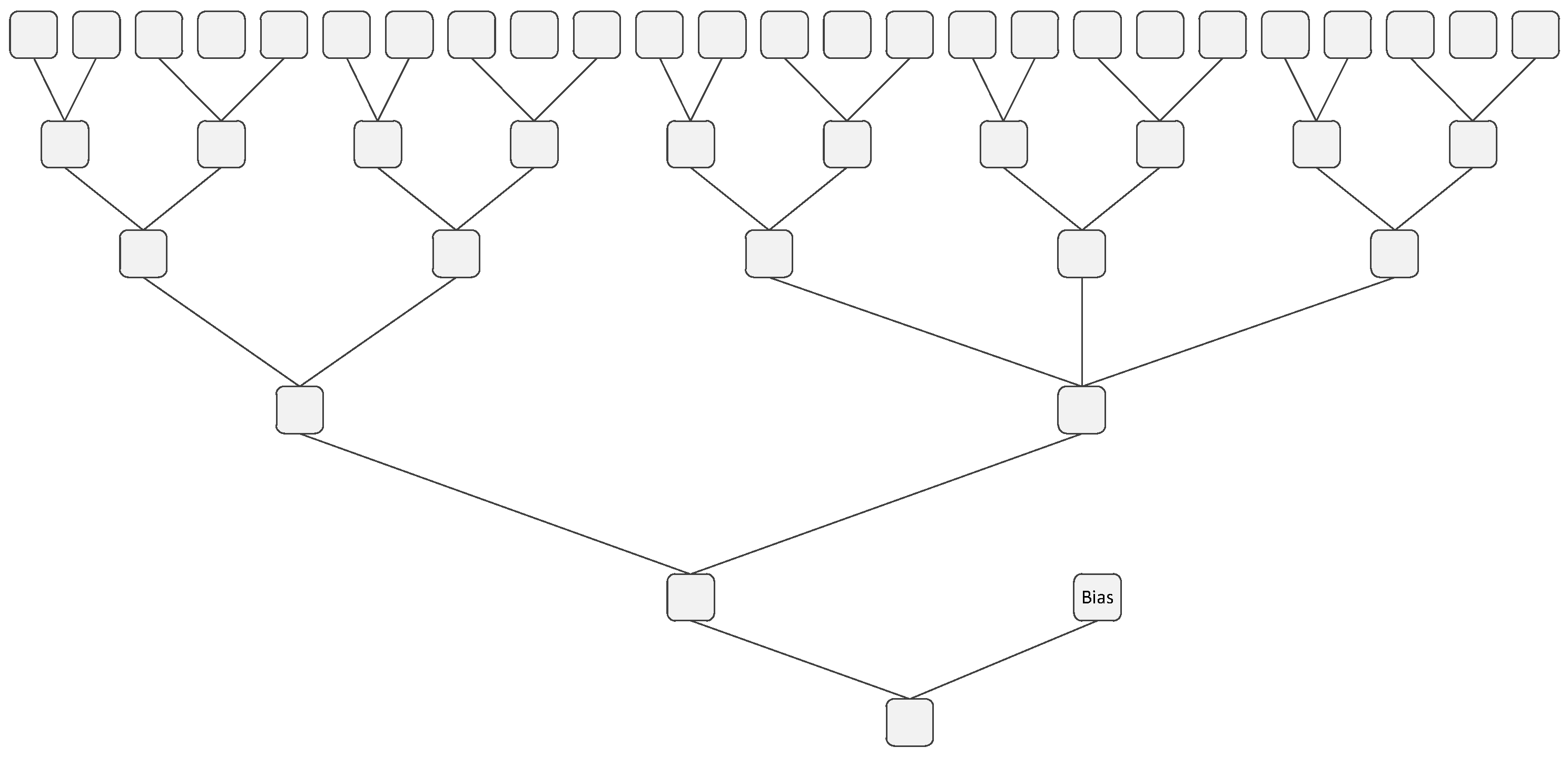
Figure 8, we can calculate how much time is needed in each layer before the next layer can start. The formula of the latency of the convolutional layers is shown in Equation (
6), where K is the size of the convolutional kernel, W is the width of the input map, and T is the clock period. Equation (
7) shows the latency of the fully connected layers and the output layers, where I is the input length. The total latency is shown in Equation (
8), where M is the number of convolutional layers and N is the number of fully connected layers and output layers. With a frequency of 250 MHz and using the ImageNet dataset, the times used in each layer of AlexNet, ZFNet, and OverFeat are shown in
Table 6.
With our structure, the theoretical latency values of AlexNet, ZFNet, OverFeat-Fast, and OverFeat-Accurate are 69.27 µs, 66.95 µs, 182.98 µs, and 132.6 µs. The longest period of time is spent in fully connected layer 2 and fully connected layer 3. This is because these fully connected layers cannot operate in parallel, and they have to wait for the former layer to finish.


