1. Introduction
On-line robotic trajectory planning, especially under dynamically changing environment settings, is a challenging core problem in the field of robotic autonomy. Many conventional robotic systems have been used in static environment scenarios such as automated factory production lines in which the off-line preplanning strategies for its paths are feasible and adequate [
1]. With recent advances in the domain of AI and reinforcement learning, however, efforts are being made to address scenarios where such assumptions do not hold.
Most conventional non-data-driven solutions for dynamic adaptive motion planning such as [
2] require considerable effort in elaborate tuning and design tailored to the system. On the other hand, many state-of-the-art systems employ deep reinforcement learning (DRL) approaches, harnessing the generalization capability of neural network models to learn the particular characteristics of the problem and the system at hand and in many cases creating end-to-end solutions [
3]. DRL approaches, however, require an extensive amount of training data which, depending on the problem, may not be feasible.
In such cases, Gaussian process (GP) regression is often explored as an alternative to DRL as it shows powerful generalization capabilities given the small amount of data. This data efficiency is especially well exploited in imitation learning scenarios, where the model must infer generalized policies from a limited number of demonstrations. However, where GP-based approaches excel in data efficiency, they are limited in data scalability, as the required matrix inversion computation becomes highly expensive as the amount of data increases [
4]. This issue extends to limitation in terms of scalability in the dimensionality of the problem, as higher dimensionality of feature space warrants a larger amount of data needed to cover the feature space. This study thus aims to address the data scalability issue of GP-based dynamic motion planning.
1.1. Literature Review
The most widely used conventional motion planners generally fall into the category of either search-based methods or optimization-based methods [
5]. Graph-based search methods [
6,
7] quantize the configuration space in graph nodes and iteratively search for the best path in the graph, while sampling-based search methods [
8,
9] iteratively create tree-like graphs from given starting points such as initial and global configurations to form a global path. While widely used for ease of implementation, these methods can become computationally expensive; are only asymptotically optimal, meaning that the paths are initially largely suboptimal; and show jerky behaviors due to the discretized nature of the methods. Local optimization in path planning has become popular for dynamic local path planning as the high computational costs of the optimization have become feasible. Timed elastic bands [
10] is a popular method as it incorporates the kinodynamic constraints of the robot into the optimization. Such methods, however, require a separate global path planner to be implemented in a hierarchical framework, and tuning the optimization parameters adds to the complexity of the planner design.
In this regard, GP-based motion planners [
11,
12,
13,
14] provide a powerful solution in that they can generalize smooth, optimal motion policies given the limited amount of initial data, which can be generated intuitively by human operators. These, however, suffer from the aforementioned limitation in terms of scalability. Such a limitation in GP-based approaches can be addressed by either improving the efficiency of the computation algorithm or employing sampling strategies that obtain only the most necessary training data. There exist several works [
4,
15,
16] that attempt to address the data scalability issue from a computational efficiency perspective.
To the authors’ knowledge, however, there has been limited research investigating data sampling methods for enhanced data efficiency and the exploration–exploitation trade-off in the GP-based imitation learning of robotic motion planning. As Gaussian process regression learning offers higher data efficiency compared to neural-network-based models, most conventional works do not focus on data sampling strategies for training their models. Refs. [
12,
13], for example, which both propose GP-based probabilistic trajectory planning frameworks for dynamic adaptation, both employ i.i.d. uniform random sampling or grid sampling approaches to obtain training data.
Especially in cases such as [
13] where the GP regression model learns optimized motion policies and thus needs to infer a reasonably optimal output for the optimization algorithm to converge to a learnable outcome, it is important to ensure that the model learns data that are learnable yet informative. One way to do so is by employing an active learning strategy, in which the data to be learned are determined by querying the model for uncertainty w.r.t. unseen data. Again, there are few works on employing active learning in GP regression models for robotic motion planning, but [
17,
18] use the learning strategy to approximate reward functions in RL quickly and in a data-efficient manner.
Voronoi tessellation, on the other hand, is classically employed in robotic path planning as a method to partition the configuration space and generate graphs of possible paths. These include methods that use generalized Voronoi diagrams [
19] to generate collision-free paths and those that employ Voronoi tessellation as a means to discretize the configuration space to apply graph search path planning [
5,
20]. Whereas such an application of Voronoi tessellation in robotic path planning has been extensively studied, there have been few efforts in its application in the learning of motion policies.
1.2. Motivation
While these methods do not extend the concept of Voronoi tessellation to sampling training features for the learning of motion planning, it can be reasoned that where these methods employ Voronoi tessellation to interpolate points between configuration space via-points and obstacles, it can also be used to interpolate points between features in higher-dimensional feature space where features represent the configuration space coordinates of via-points. Here, GP regression itself can also be interpreted as an interpolation machine that learns the correlation of input features and the outputs to find “midpoints” between learned outputs given an unseen set of features. As such, where the initial data features are conditioned to have an even spread over the feature space, Voronoi tessellation can be used to acquire features that are adequately conditioned in between the known features, such that the model can learn an even spread of data.
Hence, this nature of Voronoi tessellation as a spatial interpolation method is utilized to propose a sampling strategy that selects only the most necessary data for the GP regression model to learn, i.e., data that contribute to a relatively even distribution of learned features along the feature space.
1.3. Contribution
This study proposes a novel training scheme to address the data scalability issue of a GP regression model in dynamic robotic motion planning. This continuous-space data sampling approach uses Voronoi tessellation to leverage the spatial correlation between the input and the output of the model and balance exploration and exploitation. As baseline, Ref. [
13] provides a simple yet realistically applicable baseline experiment for a motion policy learning framework, where the model uses GP regression to infer motion policies for unseen environment configurations and consequently learns optimized versions of the inferred policies. Comparative experimental evaluation is performed to show that policies derived with the proposed method can indeed show similar optimality with fewer learned data, thereby limiting the amount of computation required for real-time inference.
3. Methods
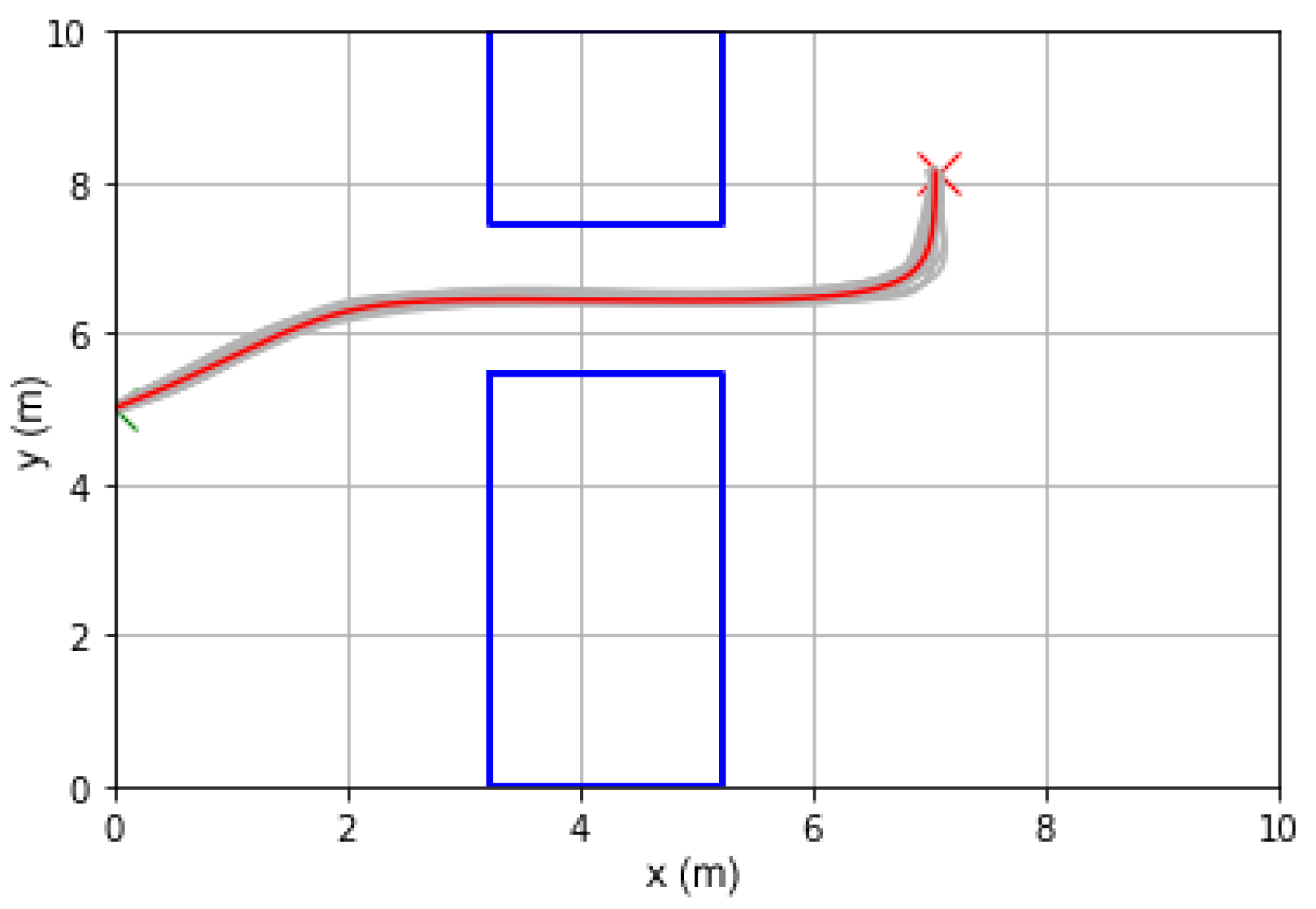
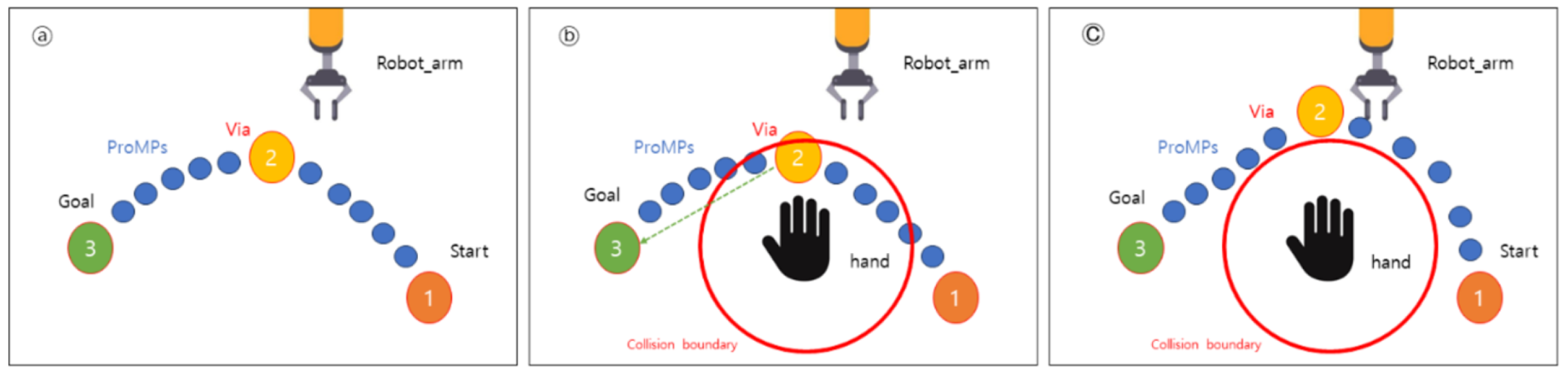
The experiment, illustrated in
Figure 1, follows the experiment detailed in Section 5.2 of Ref. [
13] (the codes can be accessed at M. Ewerton’s Github repository. URL:
https://github.com/marcoewerton/avoid_moving_walls (accessed on 19 February 2022)). As shown in
Figure 1, it involves a 2 DOF point particle agent navigating through a 2D task space, going past a via-point
at a window through a wall obstacle and terminating at the given goal position
. The starting position is fixed at
, and the 4D environment vector
is defined in the range of
,
,
,
.
Training is run for 945 iterations of an unsupervised learning loop, starting with 5 manually- generated demonstration trajectories for each of the 30 initial environment configurations. The kernel parameter as shown in Equation (
6) was defined to be
as chosen by authors of [
13].
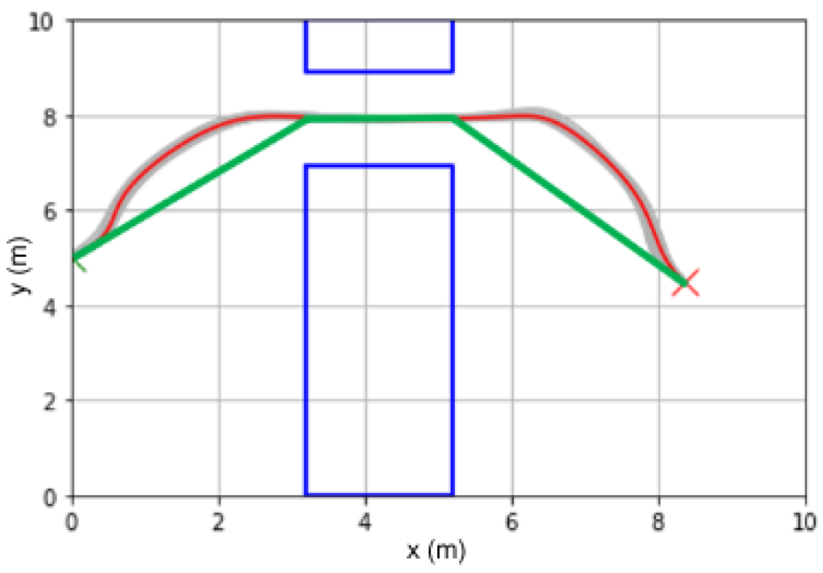
PRO uses 5 objective functions. Three of these are via-point objectives: initial position error to start configuration, minimum signed Euclidean distance to obstacle, and terminal position error to goal configuration. Two trajectory smoothing objectives are added in this experiment to be able to compare the optimality of the inferred policies. These are the average absolute value of jerk as the jerk objective function and the signed difference between the inferred trajectory and corresponding reference trajectory as the trajectory length objective function. As shown in
Figure 2, the reference trajectory (green) is automatically synthesized as three line segments between the initial position, the midpoints of the beginning and ending of the window in the wall, and the goal position.
Here, the reward function for PRO is formulated as , where denote the via-point objective, trajectory length objective weight, trajectory length objective function, jerk objective weight, and jerk objective function, respectively. The objective weights are determined to be by empirically testing over values of [0.1, 0.5, 1, 2, 5, 10] for and [, , , , ] for , except for , which is the value as set in the authors’ codes.
Additionally, the convergence and trajectory optimality criteria were relaxed in order to mitigate the additional objectives making successful convergence more difficult. A fault in the algorithm for optimization loop termination was also identified and fixed, where originally PRO would continue the optimization loop if the optimality criteria were not met even after convergence was achieved. This, with some optimization in the codes and removing redundancies, reduced the training time from 24 h or more to 6–12 h.
3.1. Baseline
The baseline approach as implemented in [
13] uses the random uniform sampling (RUS) of unseen environment features (training data).
Initial environment features for demonstration are also sampled via random uniform sampling, for which there are 5 demonstrations given for each of the 30 environment configurations. In total, 945 iterations of the self-improvement loop are set to run after which training terminates.
3.2. Voronoi Tessellation Sampling
The PRO-GP training scheme assumes that PRO can adequately optimize trajectories inferred by the GP regression model, but this is not necessarily always true. If the GP regression model cannot infer trajectories that are already adequate to a certain degree, PRO fails to converge to a learnable outcome, and nothing is learned in the iteration. This is especially so when te query feature is sampled such that it is far removed from the distribution of learned data and the model subsequently infers a highly suboptimal trajectory, which is likely during early iterations of training.
The baseline method of random uniform sampling depends on pure luck to find an environment feature to learn, which does not guarantee that the sampled data will be informative for the model. The GP regression model also requires learning an even distribution of data over the feature space to be able to yield adequate generalization performance, and random uniform sampling lacks in this regard as well.
In other words, the baseline method can often fail to find data that are similar enough to the learned data for the model to be able to learn, are dissimilar enough for them to be informative for the model, and ensure that the distribution of the learned data will converge towards an even conditioning over feature space. This poor conditioning of training data is likely to result in requiring a large amount of data before the model is able to reliably generalize over all feature space.
As such, an alternative data sampling strategy is warranted such that the exploration–exploitation trade–off is implemented to ensure that the model learns an evenly conditioned distribution of data, spanning the entire feature space, which in turn will potentially result in better inferred policies with fewer learned data. It can thus be reasoned that applying such a method will allow for the training of fewer data to yield better results.
GP regression in essence can be interpreted as a statistical interpolation method between learned features and output variables. Especially in the case of this experiment, there exists an intuitively observable spatial correlation between the input features (environment configurations) and inferred outputs (trajectory distributions) as input features dictate where in the configuration space the trajectory needs to navigate. Hence, without trying to decide the extent to which exploration should be allowed starting from a cluster of initial data, it would be possible to efficiently learn to cover the feature space by interpolating between the learned data to obtain training data features if the initial demonstration data are conditioned to be even along the feature space and cover edge cases of the feature space, where Voronoi vertices can be a good representation of such interpolation, as shown in
Figure 3.
Hence, in this experiment, a new set of demonstrations is created in 30 environment configurations sampled with Latin hypercube sampling (LHS) which enables the set of features to better represent uniform distribution than individually, independently sampled features. Using these “learned” environment features as seed points, Voronoi tessellation is performed where the obtained Voronoi vertices are the new set of environment features to be trained on. To identify the effect of initial data sampling on the end result, 5 different sets of initial demonstration data are created via random uniform sampling as per baseline, with which models are trained using Voronoi tessellation sampling (VTS) and their performances are compared to that of the model trained with initial data conditioned with LHS. The generalized algorithmic process of VTS is briefed in Algorithm 1.
| Algorithm 1: Voronoi tessellation sampling |
| Require: set of learned feature vectors D |
| Ensure: set of feature vectors to be learned V |
| Generate grid of 945 points over feature space G |
| for each point g in G do |
| Evaluate density of learned data distribution around g |
| end for |
| Add 20 grid points with lowest to D to obtain seed set S |
| Perform Voronoi tessellation with S as seeds to obtain set of Voronoi vertices V |
| for all vertices v in V do |
| Evaluate density of learned data around v |
| Evaluate closest distance to learned data around v |
| if and then |
| Delete v from V |
| end if |
| end for |
| return V |
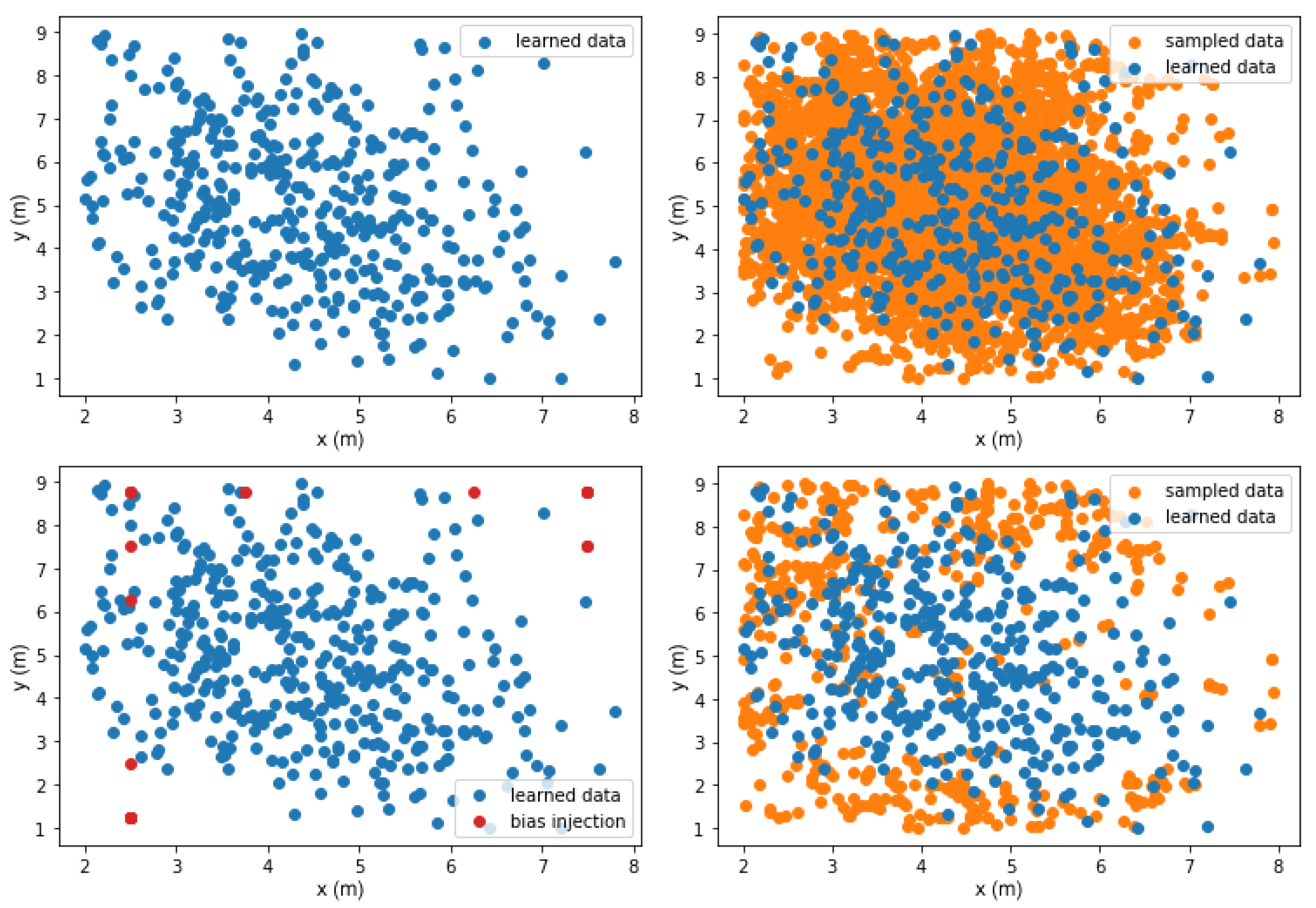
Here, two additional measures are placed to ensure effective learning—data pruning and bias injection. Sampling by interpolating alone does not ensure that the sampled features will yield inferred policies that are optimal enough for PRO to successfully converge and yet be sufficiently different from learned features that it is informative to the model. To do so, vertices (sampled features) that already have enough learned data in their vicinities are pruned before training. Here, an average Euclidean distance of 5 nearest neighboring learned data is used to measure the density of learned data around a sampled feature. Sampled features that are not within the defined feature space must also be discarded.
Furthermore, it must be noted that the interpolation-based sampling method tends to predominantly sample from within the cluster of learned data, and exploration towards the outside of the cluster is minimal if not unseen. Bias injection is thus performed when sampling, simply by adding points at relatively underexplored regions of feature space into the set of seed points.
This process is demonstrated in
Figure 4, where the data pruning and bias injection encourage gradual exploration towards the outside of the cluster of learned data and contribute to efficiently learning larger areas of the feature space. To identify the effect of data pruning and bias injection measures, a model is trained without the said procedures to be compared with control.
For this experiment, 20 grid points with lowest data density are used as injected bias seeds, and sampled features are kept to be trained on only if and , where is Euclidean distance to the closest neighboring learned data, and is the 5-NN average Euclidean distance from learned data. The number of grid points to add to the seed set and the data pruning threshold were determined empirically by inspecting 6 rounds of Voronoi tessellation sampling on the initial data without training the GP model, over the range of [5, 10, 20, 40] for the number of grid points added, [0.5, 1, 1.2, 1.5] for maximum threshold, [1, 1.2, 1.5] for minimum threshold, and [2, 2.2, 2.5, 3] for maximum threshold.
3.3. Evaluation Metrics
The outcome of each training strategy is evaluated through the optimality of the inferred policy. To measure how well the model’s trajectory inference performs, rewards (in the form of the five aforementioned objective functions, i.e., initial position error to start configuration, minimum signed Euclidean distance to obstacle, terminal position error to goal configuration, average absolute jerk, and signed trajectory length difference with synthesized reference) are evaluated for trajectories inferred in 945 environments generated from a grid of the feature space. The mean, standard deviation, minimum, and maximum of this metric will provide insight into the model’s overall performance in any given environment configuration.
5. Discussion
Results in
Table 1 are displayed in
Figure 7,
Figure 8 and
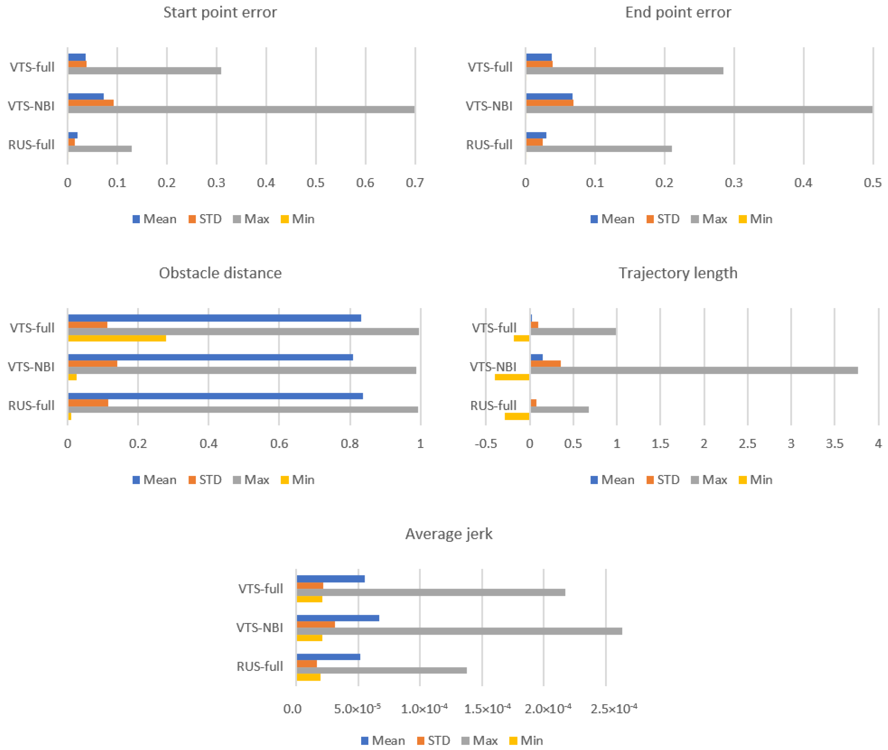
Figure 9 for ease of visual analyses. As can be seen in
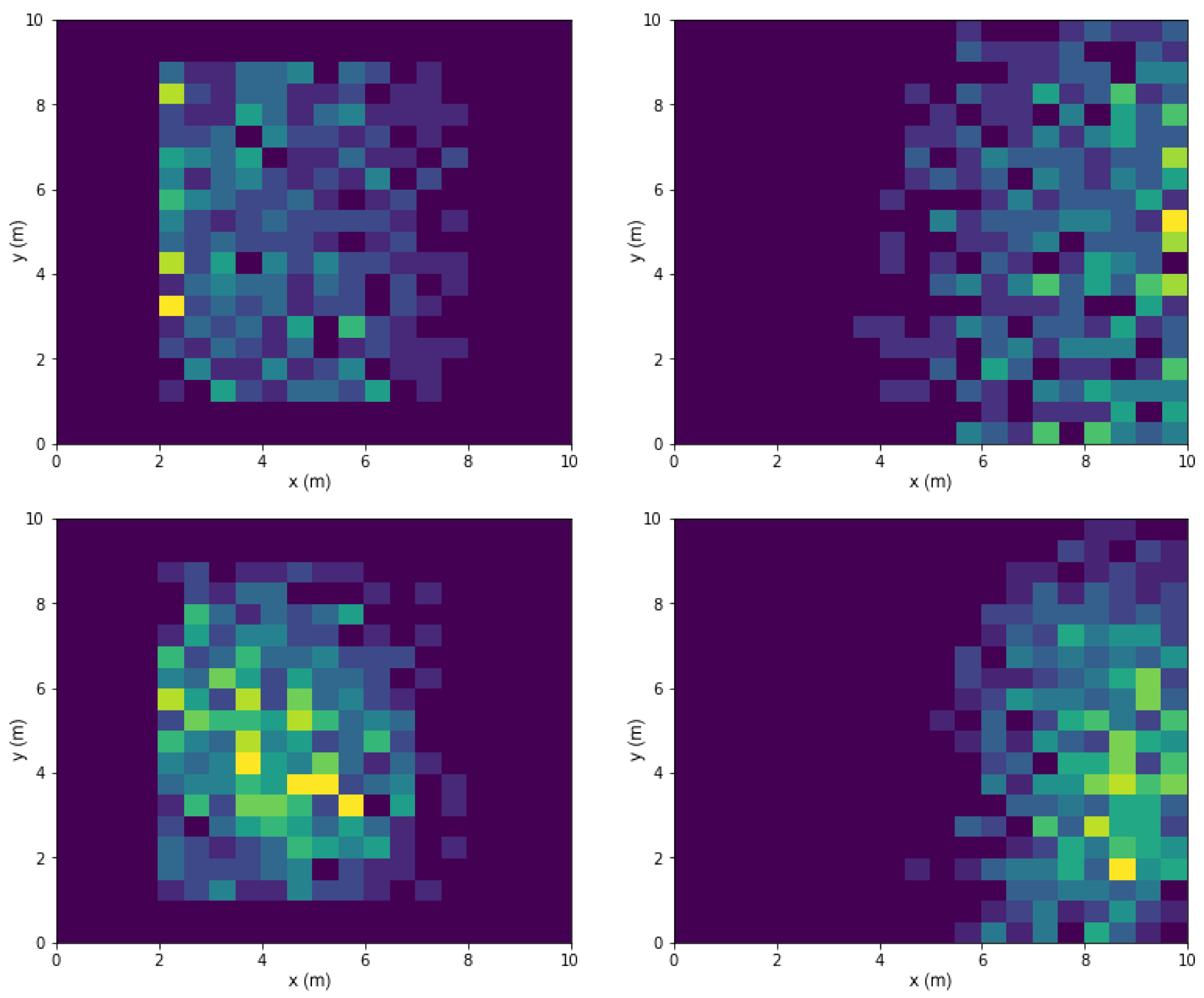
Figure 7, the proposed method (VTS-full) only manages to learn approximately 40% of the data learned by the baseline, but it achieves comparable performance. It can also be seen how the VTS model performs far worse without bias injection and data pruning measures. The reason can be identified in
Figure 10, which shows on the task space which environmental configuration features occurred most frequently as training data. Here, the learned data of VTS-NBI have clustered towards the center while VTS-full has learned to cover the feature space evenly. Where the bias injection and data pruning measures encourage exploration, the lack thereof resulted in the VTS-NBI model not being able to learn in certain regions of the feature space, thus leading to suboptimal policies.
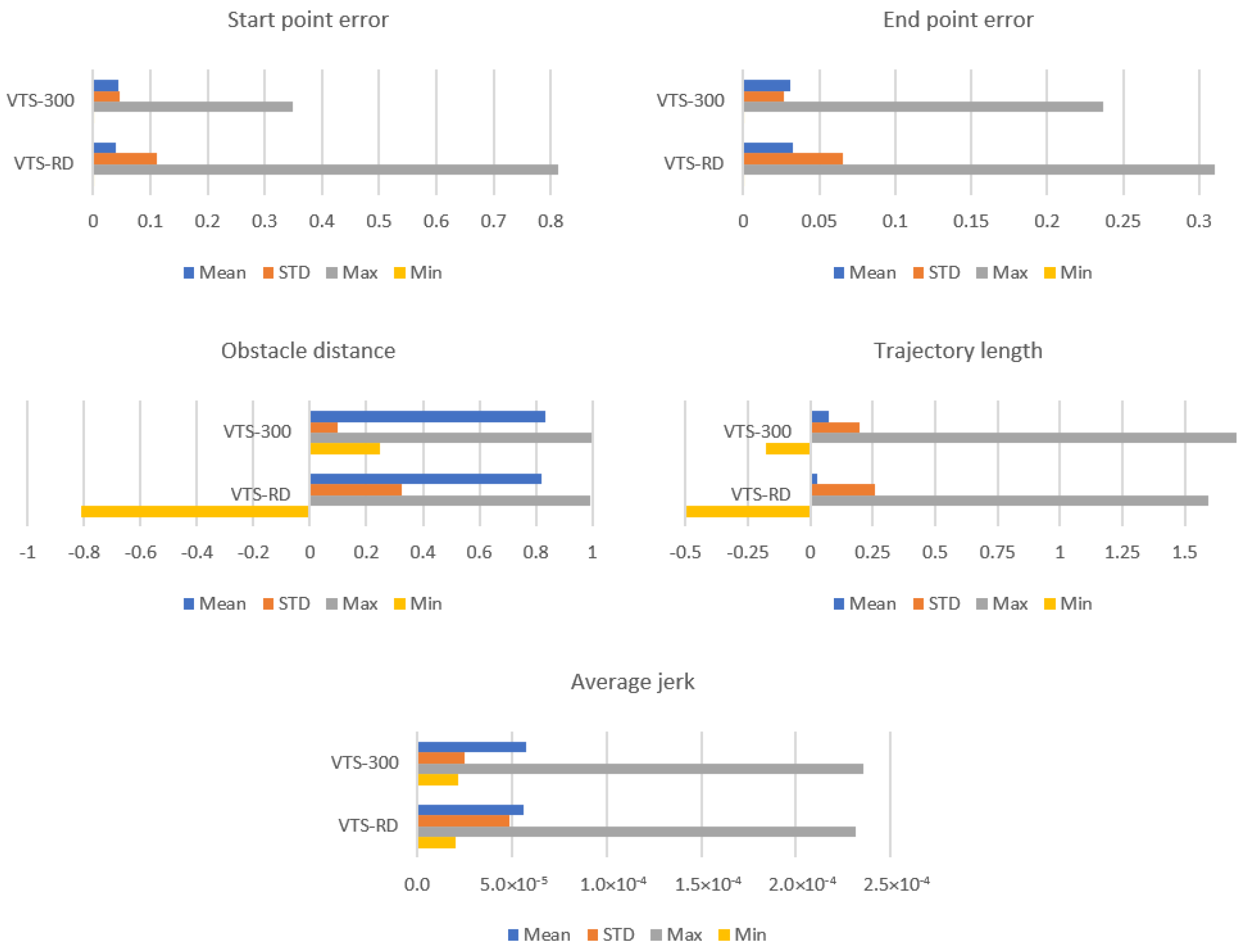
Conditioning the spread of the initial data features also proved to be important. Latin hypercube sampling was chosen to represent an ”even” spread of initial data features in the feature space in the proposed method, and
Figure 8 shows the standard proposed model (VTS-300) outperforming its counterpart (VTS-RD) with randomly selected initial data at nearly every performance metric. In particular, note the minimum obstacle distance metric, where a negative value indicates collision, rendering VTS-RD unusable in certain regions of the feature space. Note, on the other hand, in
Figure 7,
Figure 8 and
Figure 9, negative minimum values for the trajectory length objective function indicate no notable significance as outliers or undesirable behaviors, as the negative values only signify that the inferred mean trajectories are shorter than the corresponding synthesized three-segment reference trajectories shown in
Figure 2.
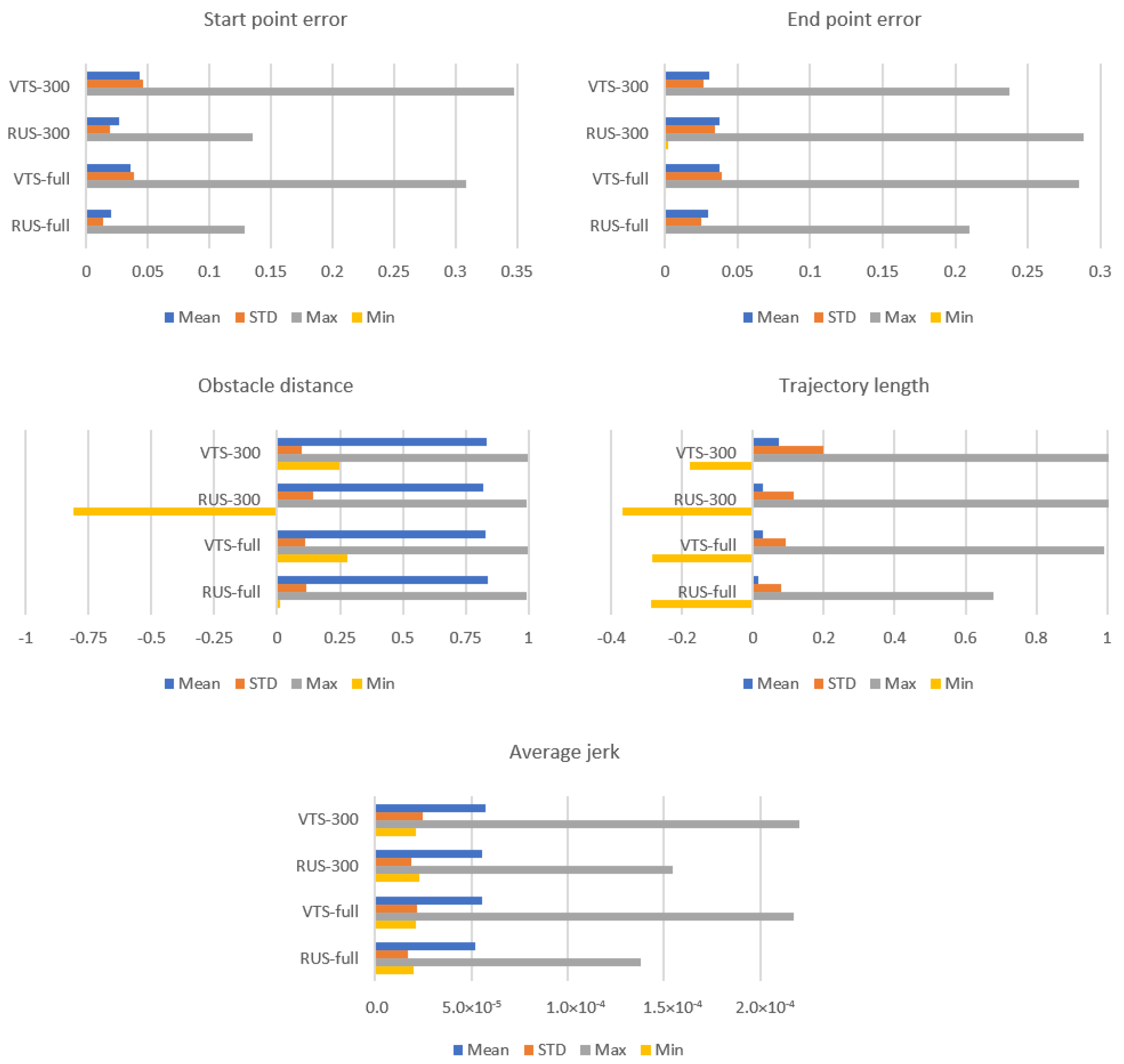
For both baseline and VTS models, early training cut-off was performed at the 300th data point learned to verify if VTS achieves a good exploration–exploitation trade-off with a small amount of data by comparing the performance of the baseline model trained with only 300 data points. For most metrics, VTS-300 achieves similar performances to VTS-full, which is worse than that of the baseline, but within a tolerable margin. Note, however, the negative minimum obstacle distance for RUS-300 in
Figure 9. This being the signed minimum distance to the obstacle, negative values mean that some inferred trajectories have collided into the obstacle, i.e., the model has failed to learn enough of the feature space to be able to reliably output an adequate, if not optimal, policy throughout all ranges of environment configurations possible.
This, when compared to the performance of VTS-300, highlights the ability of the VTS method to evenly sample across the data space while ensuring that PRO is able to optimize learnable trajectories, and it can be reasoned that by employing VTS, the GP regression model learns to reliably generalize over all feature space using fewer learned data, allowing for less computation in policy inference. In real applications, a training cut-off could be implemented, conditioned on the learning rate (amount of data learned per iteration) and ”evenness” of data distribution to automatically harness this efficiency and allow for training with fewer iterations.
Furthermore, as RUS relies on luck and a large number of iterations to reach optimal learning, it is unlikely that the optimality it learned shown in the results will extend to problems of higher DOFs as it becomes exponentially more difficult to randomly find a learnable and informative feature point. On the other hand, as VTS leverages geometric interpolation to find training data, it will likely retain the ability to reach even distribution of data along feature space.
6. Conclusions
In this study, a novel data sampling strategy for learning GP regression-based dynamic robot motion planning was proposed. This method exploits the nature of GP regression’s generalization as an interpolation technique. It allows for simple and data-efficient implementation of continuous-space data sampling for GP regression models, addressing the data scalability issue of GP regression approaches by choosing the right data to learn, and in theory is scalable to problems with higher dimensionality. Experiments show that this method can achieve similar or better policies over all feature space with fewer data compared to baseline.
While the proposed method is conceptually simple, the learning hyperparameters can be somewhat difficult to tune. Especially in the data pruning stage of VTS, there is no methodical way to determine optimal thresholds for data density measures. It is also difficult to conduct preliminary experiments with less iterations to gain insight, as the data distribution will wildly vary depending on the training outcome. These hyperparameters are, however, vital to optimal and efficient training as the restriction in these thresholds result in the algorithm prioritizing the learning of data that are more different than the learned data, thus acting as exploration–exploitation trade-off parameters. This added complexity can prove to be problematic in application to more complex scenarios.
In the future, the scalability of VTS is to be scrutinized further by exploring problem settings with higher DOFs. It would also be beneficial to explore other exploration strategies used in RL, as well as using data density metrics other than K-NN average Euclidean distance (e.g., kernel density functions).


