RenderBench: The CPU Rendering Benchmark Suite Based on Microarchitecture-Independent Characteristics

Abstract

This research addresses the issue of evaluating CPU rendering performance by introducing the innovative benchmark test suite construction method RenderBench. This method combines CPU microarchitecture features with rendering task characteristics to comprehensively assess CPU performance across various rendering tasks. Adhering to principles of representativeness and comprehensiveness, the constructed benchmark test suite encompasses diverse rendering tasks and scenarios, ensuring accurate capture of CPU performance features. Through data sampling and in-depth analysis, this study focuses on the role of microarchitecture-independent features in rendering programs, including instruction-level parallelism, instruction mix, branch prediction capability, register dependency distance, data flow stride, and memory reuse distance. The research findings reveal significant variations in rendering programs across these features. For instance, in terms of instruction-level parallelism, rendering programs demonstrate a high level of ILP (instruction-level parallelism), with an average value of 5.70 for ILP256, surpassing benchmarks such as Mibench and NAS Parallel Benchmark. Furthermore, in aspects such as instruction mix, branch prediction capability, register dependency distance, data flow stride, and memory reuse distance, rendering programs exhibit distinct characteristics. Through the application of the RenderBench method, a scalable and highly representative benchmark test suite was constructed, facilitating an in-depth exploration of CPU performance bottlenecks in rendering tasks. By delving into microarchitecture-independent features, this study provides profound insights into rendering program performance, offering valuable guidance for optimizing CPU rendering performance. The application of ensemble learning models, such as random forest, XGBoost, and ExtraTrees, reveals the significant influence of features like floating-point computation, memory access patterns, and register usage on CPU rendering program performance. These insights not only offer robust guidance for performance optimization but also underscore the importance of feature selection and algorithm choice. In summary, the results of feature importance ranking in this study provide beneficial directions and deep insights for the optimization and enhancement of CPU rendering program performance. These findings are poised to exert a positive impact on future research and development endeavors.

1. Introduction

With the rapid development of computer graphics and the emergence of diverse applications, graphics processing units (GPUs) play a crucial role in modern computer systems. Leveraging their powerful parallel computing capabilities, GPUs offer extensive support for real-time rendering, game design, virtual reality, and scientific visualization, among other domains [1,2]. Nevertheless, in the pursuit of overall system performance optimization, the role of central processing units (CPUs) remains equally significant. This is particularly pronounced for rendering tasks that necessitate close collaboration with GPUs, where CPU performance profoundly influences the efficiency and quality of the overall rendering process. In recent years, as computer architectures continue to evolve, modern CPUs have made remarkable progress in their microarchitecture and instruction sets. Nonetheless, comprehensive assessment and optimization of CPU rendering performance continue to present challenges. Traditional CPU performance evaluation methods often focus on general computing and standard benchmark tests, often overlooking features specific to rendering tasks [3,4]. Consequently, to better comprehend and optimize CPU performance in rendering, the development of a CPU rendering benchmark dataset based on microarchitecture-independent features has become paramount.

This study aims to explore and address the challenges surrounding CPU rendering performance evaluation, introducing an innovative benchmark dataset construction methodology named RenderBench. RenderBench not only incorporates CPU microarchitecture features but also integrates them with rendering task-specific characteristics to enable a comprehensive evaluation of CPU rendering performance. Guided by the principles of representativeness and comprehensiveness for the benchmark dataset, representativeness signifies that the samples included should effectively epitomize the entirety of a particular domain or problem. In this context, the benchmark dataset’s samples should encompass a wide spectrum of rendering tasks and scenarios to accurately reflect CPU performance characteristics across diverse rendering scenarios. Comprehensiveness emphasizes the dataset’s coverage scope. A comprehensive dataset should encapsulate various situations and scenes, extending beyond a singular domain or problem. In the context of rendering tasks, a comprehensive benchmark dataset should encompass a variety of rendering tasks, spanning from simple to complex, and low to high workload rendering scenarios, thus providing an encompassing understanding of CPU performance across diverse contexts. Drawing from a repository of 200 CPU rendering programs, this study utilizes the MICA microarchitecture-independent feature mining tool to conduct data sampling on 60 selected CPU rendering programs, extracting 100 microarchitecture-independent features per rendering program, subsequently followed by data analysis. On one hand, this study combined the Mibench and NPB (NAS Parallel Benchmark) CPU benchmark datasets to perform an analysis of microarchitecture-independent feature performance for the 60 selected CPU rendering programs. On the other hand, this study employed random forest importance ranking, XGBoost importance ranking, and ExtraTrees importance ranking for the 60 selected CPU rendering programs, ultimately selecting 10 performance indicators that best represent CPU rendering programs, offering insights for subsequent CPU rendering performance analysis and optimization. Simultaneously, this study conducted Pearson correlation analysis on the 60 CPU rendering programs, eliminating highly correlated rendering programs, ultimately identifying the most representative 12 CPU rendering programs as the CPU rendering benchmark dataset. The focus of this study lies in the development of a scalable, reusable, and representative benchmark dataset, enabling researchers and engineers to better understand and analyze CPU performance bottlenecks in rendering tasks.

The RenderBench methodology revolves around a spectrum of microarchitecture-independent features, encompassing the following aspects: (1). Instruction-level parallelism: This feature explores the CPU’s ability to execute multiple instructions simultaneously in rendering tasks, enhancing overall performance. High instruction-level parallelism directly influences rendering task speed and efficiency, crucial for elevating CPU rendering performance. (2). The instruction mix: Rendering tasks often involve a variety of instruction types, including arithmetic operations, logical operations, and more. Analysis of the instruction mix aids in understanding the array of operations a CPU undertakes in rendering tasks, thereby optimizing its execution flow. (3). Branch predictability: In rendering tasks, the accuracy of branch prediction greatly affects CPU performance. The strength of branch predictability determines whether the CPU can efficiently predict and execute branch statements, reducing potential performance bottlenecks. (4). Register dependency distances: Register dependencies in rendering tasks influence the execution order and parallelism of instructions. Analyzing register dependency distances assists in optimizing instruction scheduling, enhancing CPU efficiency in rendering tasks. (5). Data stream strides: Rendering tasks often involve substantial data access operations. Data storage layout and access patterns impact CPU memory access performance. Analyzing data stream strides aids in understanding CPU data access patterns during rendering, enabling targeted optimization. (6). Memory reuse distances: Memory reuse is a common occurrence in rendering tasks. Analyzing memory reuse distances allows insight into whether the CPU effectively utilizes loaded data, thereby reducing memory access latency and enhancing performance.

By delving into an in-depth analysis of these microarchitecture-independent features using the RenderBench methodology, this study comprehensively understands CPU performance in rendering tasks, providing robust support for performance optimization [5,6,7,8]. By optimizing these features, this study unearths the potential of CPUs in the realm of rendering, further enhancing the efficiency and quality of the overall rendering process, thereby propelling the continuous development of computer system performance.

2. Introduction to CPU Rendering Benchmark

The CPU rendering benchmark dataset holds significant importance in the field of computer science and engineering as a pivotal tool for assessing, comparing, and optimizing the performance of central processing units (CPUs) in rendering tasks. Firstly, the CPU rendering benchmark dataset provides an objective standard for performance evaluation and comparison. Within computer hardware and software development, comprehending the performance disparities among various CPU architectures in rendering tasks is paramount. By executing benchmark tests in a uniform testing environment, one can quantify the performance disparities among different CPUs, accurately gauging their efficiency and speed in handling rendering tasks. Secondly, the CPU rendering benchmark dataset plays a crucial role in guiding architectural design. By analyzing rendering tasks’ dependencies on distinct performance features, designers can better optimize CPU architectures to cater to the demands of the rendering domain. For instance, if rendering tasks demand higher instruction-level parallelism and branch prediction capability, designers may integrate additional execution units into the CPU architecture and optimize branch prediction strategies, thereby enhancing rendering performance. Lastly, the CPU rendering benchmark dataset can also direct future research directions and innovation. Through in-depth analysis of test outcomes, researchers can pinpoint critical issues and challenges within rendering tasks, thus guiding forthcoming research efforts and fostering the advancement of rendering technologies.

In 1989, Pixar developed an early computer system performance assessment benchmark tool called RenderMan Benchmark. This tool was specifically tailored to evaluate the performance of Pixar’s rendering engine, RenderMan, with the aim of gaining a deeper understanding of computer systems’ performance when handling complex rendering tasks. The core objective of RenderMan Benchmark is to assess the computer system’s performance during the rendering process, covering several key aspects. Firstly, concerning lighting computation performance, this benchmark explores the speed and efficiency of computer systems in handling optical effects such as lighting, shadows, and reflections under intricate lighting environments. Secondly, in terms of texture mapping performance, the benchmark focuses on the speed and accuracy of mapping textures onto object surfaces, evaluating the computer system’s performance when applying texture effects. Additionally, RenderMan Benchmark highlights geometry computation performance, scrutinizing the efficiency of handling complex geometric shapes and objects [9]. In 1991, NVIDIA introduced the Mental Ray Benchmark, designed for evaluating computer system performance using the Mental Ray rendering engine. Mental Ray is a widely used rendering engine in computer graphics and visualization, renowned for generating high-quality, realistic images, and animations [10]. In 1992, the POV-Ray community released POV-Ray (Persistence of Vision Raytracer), a powerful and extensively utilized free and open-source ray tracing rendering engine. A classic tool in the field of computer graphics, POV-Ray is predominantly employed to generate high-quality, realistic images and animations, with recognized rendering quality and flexibility across academic research, film production, and artistic creation. The unique aspect of POV-Ray lies in its utilization of ray tracing technology—a method simulating the propagation of light rays within a scene. By tracking the interaction between light rays and objects, the engine computes colors and brightness for each point in the scene. This technique yields highly realistic images, including lifelike lighting, shadows, refraction, reflection, and other [11] effects, creating visually appealing renderings closely resembling the real world. In 1995, the SPEC (Standard Performance Evaluation Corporation) introduced the first version of SPECviewperf, a benchmark tool dedicated to evaluating computer graphics system performance, specifically targeting professional 3D modeling and rendering applications. SPECviewperf tests various professional applications, providing users insights into hardware performance across a range of rendering tasks. In the realm of CPU rendering benchmark sets, SPECviewperf quantifies graphic performance through a series of visual application scenarios. These scenarios encompass 3D modeling, rendering, animation creation, and more, covering industries such as engineering, medicine, entertainment, and beyond [12].

In 2001, the YafaRay community released the YafaRay Benchmark, allowing users to run rendering tasks on different CPU hardware configurations and measure rendering time and quality. This facilitates objective assessment of various CPU performance and direct comparisons. By executing diverse rendering scenes, users acquire performance data under different workloads, gaining a better understanding of CPU capabilities in rendering tasks [13]. In 2001, Maxon Computer introduced the Cinebench benchmark tool, dedicated to evaluating computer system performance while utilizing the Cinema 4D rendering engine for image rendering. Cinema 4D is a popular 3D modeling and rendering software widely applied in film, animation, gaming, and other fields. Cinebench employs the Cinema 4D rendering engine for performance testing, reflecting real-world performance in actual application scenarios [14]. In 2005, Glare Technologies introduced the IndigoBench benchmark tool designed to evaluate computer system performance when using the Indigo Renderer rendering engine. Indigo Renderer is a physically based high-quality rendering engine widely used in film, animation, architectural visualization, and more, praised for its realistic lighting and material effects. IndigoBench results assist users in selecting suitable CPU hardware for their rendering needs and identifying hardware bottlenecks for optimization, thereby enhancing CPU rendering performance [15]. In 2009, RandomControl released the Frybench benchmark tool, specifically for evaluating computer system performance using the FryRender rendering engine. FryRender, a physically based rendering engine, is utilized extensively in film, gaming, architectural visualization, and more due to its high-quality rendering results and realism. Frybench not only tests computer system performance under FryRender but also encompasses various rendering engine features and functionalities, providing users a comprehensive understanding of rendering engine performance on different CPU hardware and in various rendering tasks [16]. In 2009, the Appleseed team introduced the Appleseed Benchmark tool, tailored for evaluating computer system performance using the Appleseed rendering engine. Appleseed, an open-source rendering engine, is widely acclaimed for its high-quality rendering results and powerful rendering capabilities. Through an array of advanced rendering algorithms and techniques, Appleseed generates high-quality, realistic rendering results, including ray tracing, global illumination, physical materials, and more. The Appleseed Benchmark evaluates CPU performance when processing these high-quality rendering algorithms, serving as a performance assessment platform [17].

In 2010, the LuxCoreRender team released the LuxMark benchmark tool, designed to assess computer system performance using the LuxCoreRender rendering engine. LuxCoreRender, an open-source rendering engine, garnered attention for its high-quality rendering results and diverse rendering functionalities. LuxMark offers various rendering modes, including ray tracing and path tracing, each with distinct characteristics and application scenarios, enabling users to tailor performance tests to their needs [18]. In 2012, Redshift Rendering Technologies introduced the Redshift Benchmark tool, focused on evaluating computer system performance while using the Redshift rendering engine. Redshift Renderer gained acclaim for its fast rendering speed and high-quality rendering results, primarily employed in visual effects, animation production, and virtual reality domains [19]. In 2014, Solid Iris Technologies released Thea Render Benchmark, specialized for assessing computer system performance using the Thea Render rendering engine. Thea Render, renowned for its rapid rendering speed and photorealistic results, is extensively used in various fields [20]. In 2014, Render Legion launched the Corona Benchmark tool, dedicated to evaluating computer system performance while using the Corona Renderer rendering engine. Corona Renderer is celebrated for its high-quality rendering results and user-friendly features, widely applied in architectural visualization, film production, and other domains [21]. In 2018, the Blender Foundation introduced the Blender Benchmark tool, tailored for evaluating computer system performance while using the Blender software for image rendering. Blender, a free and open-source 3D modeling, animation, and rendering software, is widely employed in film, animation, gaming, and more [22]. In 2018, Solid Angle released the Arnold Benchmark tool, aimed at evaluating computer system performance using the Arnold rendering engine. Arnold Renderer is distinguished for its high-quality rendering results and wide application in film, animation, and visual effects domains [23]. In 2019, OTOY launched the OctaneBench benchmark tool, specifically for evaluating computer system performance using the Octane Render rendering engine. Octane Render, a GPU-accelerated rendering engine, is recognized for its high-speed rendering efficiency and realistic results [24]. In 2021, Chaos Group released the V-Ray 5 Benchmark tool, used to assess computer system performance when using the V-Ray rendering engine. V-Ray Renderer is acclaimed for its high-quality rendering results and versatile features, widely applied in film, architecture, design, and other fields [25]. In June 2023, the Blender Foundation unveiled Blender version 3.6 LTS, supporting multiple rendering engines including Cycles, Eevee, and Workbench. Hardware-accelerated ray tracing is also supported, enabling faster rendering speeds and higher quality on compatible CPUs [26].

3. Introduction to RenderBench Microarchitecture-Independent Features

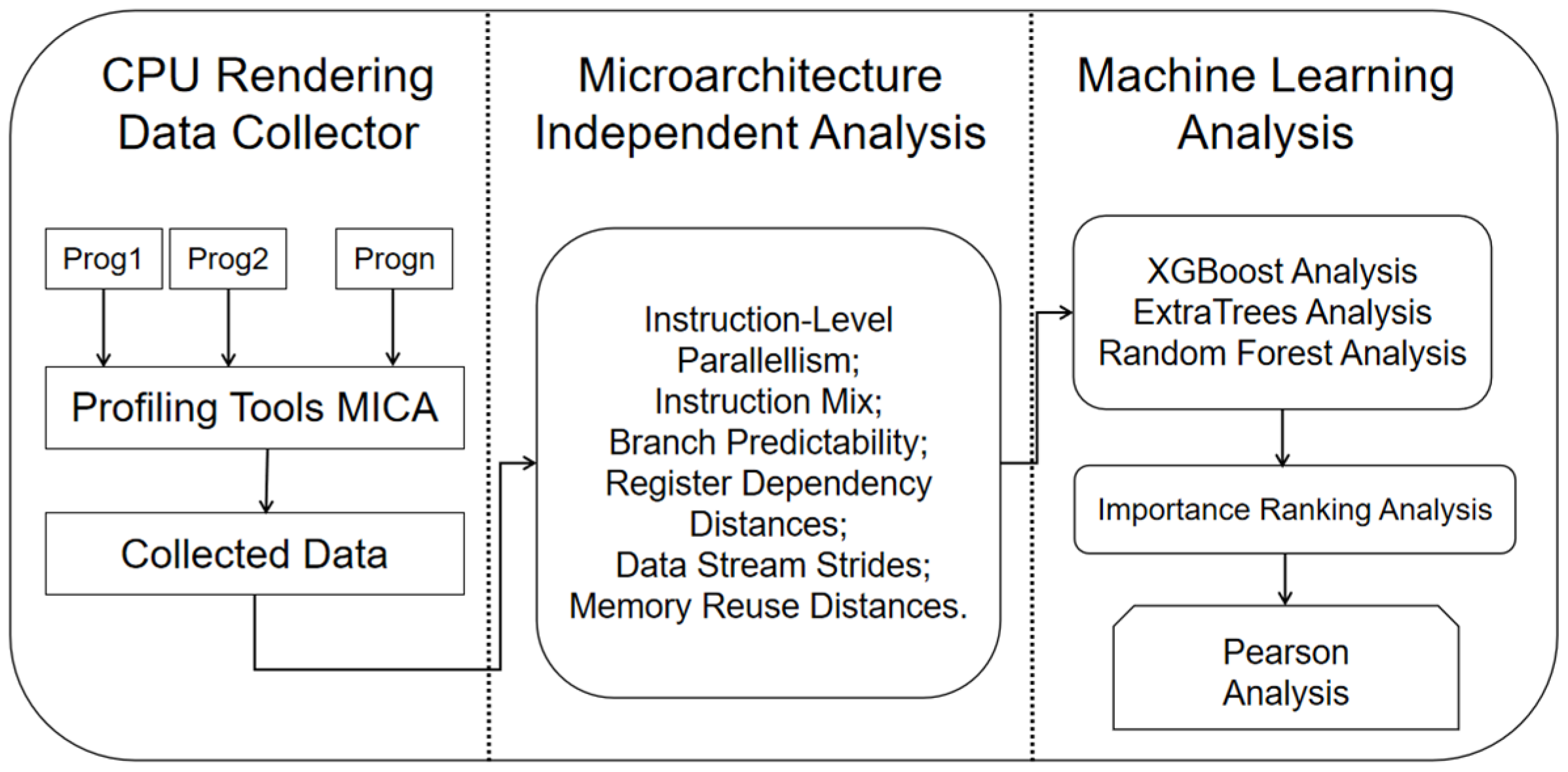
The designed CPU rendering benchmark suite, RenderBench, based on microarchitecture-independent features, comprises three main components in Figure 1: (1) Collection of CPU rendering program data, (2) microarchitecture-independent feature analysis, and (3) machine learning analysis. Firstly, in the CPU rendering program data collection phase, a selection of 120 CPU rendering programs is collected from open-source repositories. With an emphasis on the benchmark’s representativeness and comprehensiveness, the study further narrows down the selection to the most representative 60 CPU rendering programs in

Table 1. The description of CPU microarchitecture-independent characteristics.

Characteristic Name	Num	Description
Instruction-level parallelism (ILP)	4 values	IPC achievable for an idealized out-of-order processor (with perfect caches and branch predictor) for window sizes of 32, 64, 128, and 256 in-flight instructions.
Instruction mix	12 percentages	Percentage of mem read, mem write, control flow, arithmetic, floating point, stack, shift, string, MMX SSE, other, NOP and reg transfer operations.
Register dependency distances	7 probabilities	Distribution (measured in buckets) of register dependency distance, or number of instructions between production and consumption of a register instance.
Data stream strides	28 probabilities	The strides are characterized by powers of 8, i.e., 1, 8, 64, 512, 4096, 32,768, 262,144. Prob.local store stride ≤ 4096 is the portion of 0, 8, 64, 512 and 4096 in per static instruction write access. Prob.global store stride ≤ 4096 is the portion of 0, 8, 64, 512 and 4096 in all instructions write accesses. Prob.global load stride ≤ 4096 is the portion of 0, 8, 64, 512 and 4096 in all instructions read accesses.
Branch predictability	12 percentages	Branch prediction accuracy for the theoretical prediction-by-partial matching (PPM) predictor. We considered global and local history predictors, and per-address and global predictors.
Memory reuse distance	20 probabilities	The portion of the memory reuse distance is at the interval of [2n, 2n + 1], where n ranges from 0 to 18. Prob.memory reuse distance ≤ 512, namely [1, $2^9$].
Working-set size	4 numbers	Number of unique 32-byte blocks and 4-Kbyte memory pages touched for both instruction and data streams.

that encompass the entire spectrum of prevalent algorithms in the CPU rendering domain.

Concurrently, the MICA microarchitecture-independent feature extraction tool is employed to mine data from these 60 programs, capturing microarchitecture-independent features at the instruction, thread, and memory levels in

Table 2. The program names of CPU rendering programs.

Benchmark	Abr	Benchmark	Abr	Benchmark	Abr
18-RenderHelp [27]	18	19-mesh-quad [27]	19	58-raytr-master [28]	58
64-real-time-rendering [29]	64a	65-RayTracing [30]	65a	78-GameBoyEmul [31]	78
80-Cuda-Rasterizer [32]	80	88-cloud_gen [33]	88	97-ray-tracing-engine [34]	97
117-vision3D [35]	117	87-poisson_blend [36]	87	1-draw-window [37]	1a
1-tinykaboom [38]	1b	2-triangle [37]	2a	2-tinyraytracer-master [37]	2b
3 quadrangle [37]	3a	3-tinyrenderer [37]	3b	4-task04-sphere [37]	4
5-model [37]	5	15-teapot [39]	15a	15-Sample 1 Render to PNG [39]	15b
15-Sample 2—Basic App [39]	15c	15-Sample 3—Resizable [39]	15d	15-Sample 4—JavaScrip [39]	15e
15-Sample 5—File Loading [39]	15f	15-Sample6-Intro--C [39]	15g	15-Sample7-OpenGL-Integration [39]	15h
15-Sample9-Multi-Window [39]	15i	20-mesh-shading [39]	20	21 benchmarks [27]	21
22 benchmarks [27]	22	23 benchmarks [27]	23	24 benchmarks [27]	24
26-Raymarcher [40]	26	27-cartoon [41]	27	30-RayTracing [41]	30
36-pillow [42]	36	37-skinning_renderer [43]	37	38-rendertri [44]	38
42-gol3d [45]	42	43-ren [46]	43	47-render_engine [47]	47
54-PPM [48]	54a	54-Scotty3D [49]	54b	52-photon-rt-master [50]	52
62-LDSO--problem [51]	62	69-3D-RayTracer [52]	69	71-3D-Renderer [53]	71
73-nibbler-master [54]	73	78-GameOfLife-master [55]	78a	78-Gamenge-Render [56]	78b
82-raytracing-opengl [57]	82	85-DeferredRaster [58]	85	65-softbivpt [59]	65b
81-montelight-cpp [60]	81	89-voxelizer [61]	89	32-clothrendering [62]	32
64-cube-gpu-raytracing [63]	64b	33-rasterization [64]	33	31-triangles [62]	31

, thus laying the groundwork for subsequent analyses. The microarchitecture-independent feature analysis stage (2) involves an in-depth feature extraction process for the selected 60 representative CPU rendering programs, as well as non-rendering programs like Mibench and NAS Parallel Benchmark. By conducting microarchitecture-independent feature mining, the research contrasts the microarchitecture-independent attributes at the instruction, thread, and memory levels between CPU rendering and non-rendering programs. Lastly, the machine learning analysis phase (3) employs XGBoost, ExtraTrees, and random forest algorithms to rank the importance of 100 microarchitecture-independent features for each of the 60 CPU rendering programs. The resulting analysis identifies the top 10 microarchitecture-independent features that most significantly influence rendering performance, providing valuable insights for CPU rendering optimization efforts. Simultaneously, employing Pearson correlation analysis, a similarity assessment is conducted across the 60 CPU rendering programs. By considering the benchmark suite’s comprehensiveness and representativeness, a final selection of the 12 most representative CPU rendering programs is chosen as the CPU rendering benchmark suite. In our study, we utilized SPSS Statistics 29 for the purpose of data standardization. The dataset comprised 60 samples, each containing 100 microarchitecture-independent features. The primary goal of data standardization is to address potential scale differences among these features, ensuring a consistent foundation for analysis. Subsequently, we designated the variable “total instruction” as the dependent variable, while the remaining 99 features were considered independent variables. Our objective was to perform feature importance ranking through the application of machine learning techniques, specifically employing the random forest, XGBoost, and ExtraTrees algorithms. This approach allowed us to evaluate the relative significance of each independent variable concerning the dependent variable “total instruction.” Utilizing machine learning algorithms for feature importance ranking constituted a fundamental aspect of our research, enabling us to identify key factors contributing to the variability in the dependent variable. This comprehensive analysis of feature importance provides valuable insights into the relationships between microarchitecture-independent features and “total instruction,” ultimately enhancing our understanding of our research objectives.

3.1. Analysis of Instruction-Level Parallelism Feature

Instruction-level parallelism (ILP) is a crucial concept within computer architecture, elucidating the capability for multiple instructions to execute concurrently during program execution. The presence of ILP allows processors to more efficiently harness computational resources, thereby enhancing program execution speed and performance. Measurement of ILP, using MICA, typically involves considering various instruction window sizes, denoting the number of instructions that can be simultaneously processed.

Here, this study considers four different instruction window sizes: 32, 64, 128, and 256. The choice of instruction window size directly affects the processor’s ability to execute instructions in parallel, with larger windows accommodating more instructions, thereby enhancing parallelism and performance. While measuring ILP, certain ideal conditions are assumed, such as perfect caching and branch prediction. This simplifies the measurement process to make the impact on ILP assessment more apparent. However, in real-world scenarios, cache might not perfectly store all data, and branch prediction might not be entirely accurate, potentially limiting actual ILP. The constraints of ILP primarily stem from instruction window size and data dependencies. The instruction window’s size dictates the number of instructions that can be executed concurrently. An insufficiently sized window may underutilize processor resources, leading to performance bottlenecks. Data dependencies refer to the interconnections between instructions. If data dependencies exist, certain instructions might have to wait for others to complete before execution, thereby diminishing ILP.

This study conducted instruction-level parallelism analysis on 60 CPU rendering programs, 30 NAS Parallel Benchmarks, and 30 Mibench programs. As depicted in Figure 2, the average ILP32, ILP64, ILP128, and ILP256 values for the 60 CPU rendering programs were 4.29, 4.94, 5.42, and 5.70, respectively. The ILP for each instruction window size surpassed that of the 30 NAS Parallel Benchmarks and 30 Mibench programs by one unit. Larger instruction windows can more efficiently exploit program parallelism, thereby enhancing performance. Taking actual rendering programs as an example, consider a complex scene rendering task involving extensive texture mapping and lighting computations. With a smaller instruction window (e.g., ILP32), data dependencies might limit ILP due to operations like texture mapping and lighting computations. However, within a larger instruction window (e.g., ILP256), more parallel operations can be accommodated, thereby expediting the execution of texture mapping and lighting computations. Furthermore, a larger instruction window can more effectively handle operations like branch prediction and memory access, further boosting rendering program performance. Rendering programs generally exhibit higher ILP values than non-rendering programs, as they frequently involve substantial parallel computations, such as lighting calculations, texture mapping, and polygon processing. These computations inherently possess strong data independence, allowing multiple pixels or fragments to be processed simultaneously. In contrast, certain applications within the NAS Parallel Benchmarks and Mibench suite might be more limited by data correlations, resulting in constrained ILP. Parallel computations within rendering programs can effectively achieve ILP within larger instruction windows. For instance, during the lighting calculation phase, multiple intersection points of light rays can be computed concurrently, potentially without data dependencies. Conversely, some applications in the NAS Parallel Benchmarks and Mibench suite might include more conditional branches and loops, which could impede ILP realization. Rendering programs often exhibit favorable data access patterns, enabling memory access to overlap within larger instruction windows. For instance, during the texture mapping phase, multiple pixels might need to access the same texture data. This data access pattern permits simultaneous execution of multiple memory access instructions within the instruction window, thereby enhancing ILP. Conversely, some applications within the NAS Parallel Benchmarks and Mibench suite might possess irregular memory access patterns, constraining ILP realization.

3.2. Analysis of Instruction Mix Characteristics

Instruction mix is one of the essential metrics in the performance evaluation of computer architectures, illustrating the relative proportions of various types of instructions during program execution. In this study, the Intel profiling tool PIN, combined with the microarchitecture feature extraction tool MICA, was employed to categorize instructions based on the X86 instruction set manual. A total of 11 instruction types were identified, including mem-read, sse, mem-write, nop, stack, control-flow, floating-point, shift, string, and other types. These 11 instruction types encompassed in the instruction mix feature represent the diversity of programs. Let i denote the index of instruction types (e.g., i = 1 for mem-read, i = 2 for sse, and so on). You can use the following formula to express the percentage of each instruction type in instruction mix:

$$P(i)=\frac{N\left(i\right)}{N\left(total\right)}\times \mathrm{100\%}$$

(1)

where P(i) is the percentage of instruction type i, N(i) is the count of instruction type i in the program, and N(total) is the total count of instructions in the program. Different applications may exhibit varying demands and proportions for these instruction types. For instance, floating-point instructions might dominate in compute-intensive applications, while mem-read and mem-write instructions could be more crucial in memory-intensive applications. The diversity of instruction types allows the instruction mix to comprehensively depict the performance characteristics and requirements of programs. In Figure 3, analyzing the instruction mix of CPU rendering programs reveals that control-flow and arithmetic instructions account for a significant proportion among the 60 CPU rendering programs, with average percentages of 42.43% and 12.34%, respectively. This indicates a substantial demand for control flow operations and arithmetic computations in CPU rendering tasks.

Furthermore, the average percentages of mem-read and mem-write instructions are also significant, at 19.03% and 9.57%, respectively, indicating a notable demand for memory access and data writing within rendering programs. In comparison with Mibench and NAS Parallel Benchmark in Figure 4 and Figure 5, it is evident that CPU rendering programs exhibited higher demand for control-flow and arithmetic instructions. In contrast, Mibench showed a higher proportion of arithmetic and floating-point instructions, while NAS Parallel Benchmark demonstrated greater demand for mem-read and MMX/SSE instructions. This suggests that CPU rendering programs prioritize control flow operations and arithmetic computations in alignment with the nature of rendering tasks. Additionally, the demand for stack, shift, and string instructions within CPU rendering programs is relatively low, implying that these instruction types do not play a dominant role in rendering tasks. Moreover, the proportion of NOP and reg-transfer instructions within CPU rendering programs is also modest, possibly indicating a focus on practical computations and data operations rather than relying heavily on no-operation or register transfer operations. Analyzing the instruction mix can assist developers in better optimizing and balancing the instruction flow of programs. By adjusting the ratios of different instruction types, it is possible to optimize program performance on specific architectures. For instance, in a memory-intensive application, optimizing the ratio of mem-read and mem-write instructions could alleviate memory access bottlenecks. Such optimization and balancing can lead to improved performance across various architectures.

3.3. Analysis of Register Dependency Distances Feature

Register dependency distance refers to the dynamic number of instructions generated between the write and subsequent read of a data from the same register during program execution. This concept is closely associated with computer architecture, particularly in the context of instruction-level parallelism (ILP), and is particularly pertinent to superscalar and out-of-order execution processor architectures. In such architectures, processors can execute multiple instructions simultaneously. However, the presence of register dependencies can lead to out-of-order execution and reordering of instructions, thereby impacting program performance.

$$RDD=R-W$$

(2)

where RDD is the register dependency distance, R is the index of the instruction that reads from the same register, and W is the index of the instruction that writes to the same register. Register dependency distance is a pivotal performance metric within computer architecture research. A shorter register dependency distance typically indicates that instructions within a program can execute faster, as data can be read from registers more swiftly, consequently reducing instruction wait times. Conversely, a longer register dependency distance can extend instruction waiting times, thereby diminishing program execution efficiency. The register dependency distance is influenced by the data dependency relationships within a program. When one instruction needs to wait for the result of another instruction, register dependency distance arises. If a program contains a substantial number of data dependencies, resulting in a larger register dependency distance, the processor might be unable to fully leverage instruction-level parallelism, consequently impairing program performance.

As illustrated in Figure 6, the horizontal axis, namely reg_depend_1, reg_depend_2, reg_depend_4, reg_depend_8, reg_depend_16, reg_depend_32, and reg_depend_64, respectively denote the percentage of dynamic instructions generated between multiple register writes and reads in relation to the total number of instructions. In the realm of register dependency distances, measurements have been conducted for CPU rendering programs, Mibench, and NAS Parallel Benchmark, with average values provided for distinct register dependency distances. Firstly, it can be observed that as register dependency distance increased, all three benchmark programs exhibited an escalating trend in register dependency distance. This implies that with heightened occurrences of data utilization within registers, inter-instruction dependency relationships also proliferate. Larger register dependency distances lead to augmented instruction waiting times, consequently diminishing program performance. Contrasting the outcomes of the three benchmark programs, it becomes apparent that CPU rendering programs marginally exceeded Mibench and NAS Parallel Benchmark in terms of register dependency distance. This indicates a more substantial prevalence of data dependency relationships among instructions in the test cases of CPU rendering programs, resulting in frequent use of data stored in registers, thereby elevating the register dependency distance. Furthermore, it is noteworthy that the register dependency distances of all three benchmark programs increased to varying degrees as register dependency distance expanded. This underscores the notion that with heightened data utilization occurrences within registers, inter-instruction data dependency relationships also escalate. In actual program scenarios, fluctuations in register dependency distance might be influenced by a multitude of factors, including the program’s data access patterns, loop structures, and conditional branches.

3.4. Analysis of Data Stream Strides Feature

Data stream strides refer to the distances between adjacent memory accesses within a data stream, encompassing local load (memory read) strides, global load (memory read) strides, local store (memory write) strides, and global store (memory write) strides. ‘Local’ pertains to the stride of each static instruction access, while ‘global’ refers to the average stride of all instructions. These strides are characterized using powers of 8, typically ranging from 0, 8, 64, 512, 4096, 32,768, to 262,144. Data stream strides measure the continuity and locality of memory access, with smaller strides indicating more contiguous and localized memory access, thus enhancing data access efficiency and performance. Conversely, larger strides may result in increased memory access latency and cache misses, leading to reduced program performance.

Local Load (Memory Read) Stride (LS_local):

$$\mathrm{L}\mathrm{S}\_\mathrm{l}\mathrm{o}\mathrm{c}\mathrm{a}\mathrm{l}\left(\mathrm{i}\right)=\mathrm{A}\mathrm{d}\mathrm{d}\mathrm{r}\mathrm{e}\mathrm{s}\mathrm{s}\left(\mathrm{i}\right)-\mathrm{A}\mathrm{d}\mathrm{d}\mathrm{r}\mathrm{e}\mathrm{s}\mathrm{s}(\mathrm{i}-1)$$

(3)

where i represents the instruction index, and Address(i) is the memory address accessed by the ith instruction.

Global Load (Memory Read) Stride (LS_global):

$$\mathrm{L}\mathrm{S}\_\mathrm{g}\mathrm{l}\mathrm{o}\mathrm{b}\mathrm{a}\mathrm{l}=\mathrm{A}\mathrm{v}\mathrm{e}\mathrm{r}\mathrm{a}\mathrm{g}\mathrm{e} \mathrm{o}\mathrm{f} \mathrm{a}\mathrm{l}\mathrm{l} \mathrm{L}\mathrm{S}\_\mathrm{l}\mathrm{o}\mathrm{c}\mathrm{a}\mathrm{l}\left(\mathrm{i}\right) \mathrm{f}\mathrm{o}\mathrm{r} \mathrm{i}=1 \mathrm{t}\mathrm{o} \mathrm{N}$$

(4)

where N is the total number of instructions in the program.

Local Store (Memory Write) Stride (SS_local):

$$\mathrm{S}\mathrm{S}\_\mathrm{l}\mathrm{o}\mathrm{c}\mathrm{a}\mathrm{l}\left(\mathrm{i}\right)=\mathrm{A}\mathrm{d}\mathrm{d}\mathrm{r}\mathrm{e}\mathrm{s}\mathrm{s}\left(\mathrm{i}\right)-\mathrm{A}\mathrm{d}\mathrm{d}\mathrm{r}\mathrm{e}\mathrm{s}\mathrm{s}(\mathrm{i}-1)$$

(5)

where i represents the instruction index, and Address(i) is the memory address accessed by the ith instruction.

Global Store (Memory Write) Stride (SS_global):

$$\mathrm{S}\mathrm{S}\_\mathrm{g}\mathrm{l}\mathrm{o}\mathrm{b}\mathrm{a}\mathrm{l}=\mathrm{A}\mathrm{v}\mathrm{e}\mathrm{r}\mathrm{a}\mathrm{g}\mathrm{e} \mathrm{o}\mathrm{f} \mathrm{a}\mathrm{l}\mathrm{l} \mathrm{S}\mathrm{S}\_\mathrm{l}\mathrm{o}\mathrm{c}\mathrm{a}\mathrm{l}\left(\mathrm{i}\right) \mathrm{f}\mathrm{o}\mathrm{r} \mathrm{i}=1 \mathrm{t}\mathrm{o} \mathrm{N}$$

(6)

where N is the total number of instructions in the program, similar to LS_global but for memory write instructions.

These formulas provide a conceptual understanding of how to calculate these strides. You would need to analyze the memory access patterns of instructions within a program to calculate these values. The key is to determine the memory address accessed by each instruction and then compute the differences between consecutive memory accesses to measure the stride.

The ‘local’ stride indicates the distance between memory accesses of each static instruction, while the ‘global’ stride represents the average distance between memory accesses for all instructions. Strides are characterized using powers of 8, including 0, 8, 64, 512, 4096, 32,768, and 262,144. These power values correspond to memory address offsets, for example, 8 denotes a difference of 8 bytes between memory addresses, and 64 denotes a difference of 64 bytes. This characterization method aids in effective statistical analysis of memory access patterns. Data stream strides hold significance in understanding program memory access patterns and performance optimization. Smaller local and global strides typically indicate better memory access continuity and locality, facilitating performance improvement through sensible cache optimization. Conversely, larger strides may lead to scattered and discontinuous memory access, necessitating targeted optimizations to reduce memory latency and enhance performance.

From the data in Figure 7, it is evident that the CPU rendering programs, Mibench, and NPB benchmark exhibited varying average values under different local memory read strides. Their average values for stride_0 (stride of 0) were exceedingly small, almost approaching 0. This is likely because adjacent memory reads with a stride of 0 are rare in practical programs. With increasing stride values, the average values gradually rose, indicating growing distances between adjacent memory reads and diminishing data access locality. When comparing CPU rendering programs with other test programs, it was observed that CPU rendering programs generally had smaller average values under different strides, particularly under stride_0 and stride_8. This suggests that CPU rendering programs possess better local and contiguous memory access in terms of memory reads. In contrast, Mibench and NPB benchmark exhibited slightly larger average values under the same strides, implying somewhat lower memory read locality compared to CPU rendering programs. As strides increased, the average values for all test programs progressively increased, aligning with expectations. Larger strides signify greater distances between adjacent memory reads, reduced data locality, and possibly heightened cache misses, affecting program performance.

Similarly, CPU rendering programs, Mibench, and NPB benchmark displayed varying average values under different global memory write strides. Their average values for stride_0 were extremely small, nearly reaching 0, indicating infrequent occurrence of adjacent memory writes with a stride of 0 in practical programs. As stride values increased, the average values gradually rose, implying larger distances between adjacent memory writes and diminishing data access locality. CPU rendering programs tended to have smaller average values under different strides, especially under stride_0 and stride_8. This implies that CPU rendering programs exhibit better local and contiguous memory access in terms of memory writes. In comparison, Mibench and NPB benchmark exhibited slightly larger average values under the same strides, indicating somewhat lower memory write locality compared to CPU rendering programs. As strides increased, the average values for all test programs increased consistently, aligning with expectations. Larger strides denote greater distances between adjacent memory writes, reduced data locality, and potential increases in cache misses, thereby influencing program performance.

3.5. Analysis of Branch Predictability Feature

In the context of this program, the present study conducted an assessment of predictive performance of conditional branches utilizing the MICA feature mining tool, employing a methodology termed prediction-by-partial-match (PPM) predictor. This predictor leverages the historical occurrences of past conditional branches and employs a localized matching approach to forecast outcomes of branch instructions. The evaluation process encompassed four distinct configurations, involving global/local branch history and employment of shared/independent prediction tables, coupled with three varying historical lengths (4, 8, 12 bits).

PPM context probability formula: This formula calculates the probability of a specific symbol (e.g., a character in text compression) given the context (previous symbols).

$$\mathrm{P}\left(\mathrm{s}\mathrm{y}\mathrm{m}\mathrm{b}\mathrm{o}\mathrm{l}\right|\mathrm{c}\mathrm{o}\mathrm{n}\mathrm{t}\mathrm{e}\mathrm{x}\mathrm{t})=(\mathrm{C}\mathrm{o}\mathrm{u}\mathrm{n}\mathrm{t}(\mathrm{c}\mathrm{o}\mathrm{n}\mathrm{t}\mathrm{e}\mathrm{x}\mathrm{t},\mathrm{s}\mathrm{y}\mathrm{m}\mathrm{b}\mathrm{o}\mathrm{l})+1)/(\mathrm{C}\mathrm{o}\mathrm{u}\mathrm{n}\mathrm{t}\left(\mathrm{c}\mathrm{o}\mathrm{n}\mathrm{t}\mathrm{e}\mathrm{x}\mathrm{t}\right)+\mathrm{N})$$

(7)

where P(symbol|context) is the conditional probability of the symbol given the context, Count(context, symbol) is the count of occurrences of the symbol following the context, and Count(context) is the count of occurrences of the context. N is the total number of symbols in the alphabet.

PPM update formula: In the PPM algorithm, probabilities are updated based on observed data. The update formula is typically used to adjust probabilities after each symbol is encoded or decoded.

$$\mathrm{N}\mathrm{e}\mathrm{w} \mathrm{p}\mathrm{r}\mathrm{o}\mathrm{b}\mathrm{a}\mathrm{b}\mathrm{i}\mathrm{l}\mathrm{i}\mathrm{t}\mathrm{y}=\mathsf{\alpha }\ast \mathrm{o}\mathrm{b}\mathrm{s}\mathrm{e}\mathrm{r}\mathrm{v}\mathrm{e}\mathrm{d} \mathrm{p}\mathrm{r}\mathrm{o}\mathrm{b}\mathrm{a}\mathrm{b}\mathrm{i}\mathrm{l}\mathrm{i}\mathrm{t}\mathrm{y}+(1-\mathsf{\alpha })\ast \mathrm{p}\mathrm{r}\mathrm{i}\mathrm{o}\mathrm{r} \mathrm{p}\mathrm{r}\mathrm{o}\mathrm{b}\mathrm{a}\mathrm{b}\mathrm{i}\mathrm{l}\mathrm{i}\mathrm{t}\mathrm{y}$$

(8)

where New probability is the updated probability of a symbol, α (alpha) is a weighting factor between 0 and 1 that determines the influence of the observed probability, Observed probability is the probability estimated from observed data, and Prior probability is the probability from the previous iteration [65]. These formulas are fundamental to understanding how PPM predictors work, particularly in the context of data compression and prediction modeling. The specific implementation details may vary depending on the variant of the PPM algorithm being used. Additionally, average execution and transition counts were quantified. The PPM predictor constitutes a machine learning-based approach, with the aim of predicting future outcomes of conditional branches based on their historical occurrence patterns. By dissecting patterns within the branch history, the PPM predictor endeavors to identify recurring sequences and enhance prediction accuracy. The evaluation encompassed four configurations:

Global branch history: In this configuration, the PPM predictor utilized global branch history, thereby considering the collective historical data of all program branches for predictions.

Local branch history: In contrast, the local branch history configuration treated each branch individually, utilizing distinct historical information for predictions.

Shared prediction table: Certain configurations employed shared prediction tables, where multiple branches shared the same prediction table for forecasting.

Independent prediction table: Alternatively, other configurations assigned independent prediction tables for each branch, ensuring prediction information specific to each individual branch.

Furthermore, the MICA feature mining tool incorporated three distinct historical lengths: 4 bits, 8 bits, and 12 bits. Longer historical lengths have the potential to capture more intricate branch behavior patterns, possibly leading to enhanced prediction accuracy. During the evaluation process, average execution and transition counts were also gauged. Average execution denotes the proportion of executed branches during program execution, including jumps or loops. Transition count indicates the frequency of transitions in branch instructions, switching from execution to non-execution or vice versa. Through the implementation of varied configurations and historical lengths in the evaluation, a comprehensive understanding of the PPM predictor’s performance and accuracy was achieved. The objective was to identify the most effective prediction configurations, while also comprehending the impact of branch history length on prediction accuracy. This information is pivotal for optimizing branch prediction mechanisms and augmenting overall program performance.

Within the context of the CPU rendering program in Figure 8, different branch prediction configurations (GAg and PAg) were employed, alongside distinct historical lengths (4 bits, 8 bits, 12 bits), to measure misprediction counts in branch prediction. Concurrently, two distinct branch prediction configurations, GAg and PAg, were employed. GAg denotes the global adaptive predictor, which utilizes global historical data to forecast branch instruction execution paths. PAg signifies the local adaptive predictor, which predicts branch instruction execution paths based on the historical information of each individual branch. Additionally, distinct historical lengths (4 bits, 8 bits, 12 bits) were employed. Historical length indicates the number of bits in the historical record used for branch prediction. The results illustrate that misprediction counts increase with the augmentation of historical length. This phenomenon can be attributed to longer historical lengths potentially resulting in more intricate prediction patterns, which in turn may contribute to increased mispredictions. Furthermore, during the transition from the GAg to PAg predictor, misprediction counts also exhibited an increase. This was due to the distinct prediction strategies employed by these two predictors, potentially resulting in varied prediction accuracies for diverse branch instructions.

Comparatively, in contrast to the CPU rendering program, Mibench demonstrated fewer instances of misprediction. This can be attributed to the relatively simpler branch instruction patterns within Mibench. In this case, shorter historical lengths were sufficient to address the majority of branch prediction requirements, thereby minimizing the significance of longer historical lengths in performance enhancement. In the comparison between the GAg and PAg predictors, it was observed that the GAg predictor exhibited relatively higher misprediction counts at shorter historical lengths, which gradually diminished as historical length increased. This suggests that the predictive capability of the GAg predictor might be limited for shorter historical lengths, whereas its predictive accuracy improves with increasing historical length. In contrast, the PAg predictor exhibited greater stability across different historical lengths, manifesting relatively fewer instances of misprediction. Compared to the CPU rendering program and Mibench, the NPB benchmark demonstrated a higher frequency of mispredictions. This could be attributed to the complexity of programs within the NPB benchmark, encompassing a greater number of branch instructions and consequently presenting greater challenges in branch prediction. In the comparison between GAg and PAg predictors within the NPB benchmark, it was evident that across all historical lengths, the GAg predictor displayed higher misprediction counts than the PAg predictor. This underscores the weaker predictive capacity of the GAg predictor for the NPB benchmark, particularly in predicting complex branch instruction patterns. Conversely, the PAg predictor exhibited greater stability. With the increase in historical length, both GAg and PAg predictors exhibited an augmentation in misprediction counts. This illustrates that for intricate programs within the NPB benchmark, augmenting historical length does not fully resolve the challenges associated with branch prediction, and a degree of misprediction still persists.

3.6. Analysis of Memory Reuse Distances Feature

In the chart shown based on a Kiviat diagram in Figure 9, various metrics related to memory reuse distance are presented, along with their proportions within the total reuse distance. Here, memory reuse distance refers to the count of times a program accesses different 64-byte cache blocks after accessing the same one. To grasp this concept better, one can analogize it to the behavior of a processor running a program: after initially accessing a 64-byte cache block, the processor might subsequently access two or three other distinct 64-byte cache blocks before returning to the original block. The memory reuse distance quantifies the number of cache block accesses made by the processor during this process. The chart displays eight distinct metrics (m1, m2, …, m8), representing the proportions of memory reuse distances within different ranges concerning the total reuse distance. Specifically, m1 denotes the proportion of memory reuse distances in the range of 0 to 4 bytes, m2 signifies the proportion in the range of 4 to 16 bytes, and so forth. The values of these metrics fall between 0 and 1, with the left boundary of each interval excluded and the right boundary included. For instance, if m1 is 0.5, it implies that the portion of reuse distances within 0 to 4 bytes accounts for 50% of the total reuse distance. Similarly, if m2 is 0.3, it indicates that the portion of reuse distances within 4 to 16 bytes constitutes 30% of the total reuse distance. These metrics aid in understanding the memory access patterns of a program across different reuse distance ranges. Such analysis is pivotal for optimizing program performance, as insights into memory reuse distance characteristics enable targeted optimization of memory access patterns, thus enhancing execution efficiency and performance. For instance, if a high access proportion is observed within a specific memory reuse distance range, measures can be taken to reduce memory access instances, such as increasing cache size or optimizing data structure layout. Such optimizations mitigate memory access latencies, thereby improving program execution speed. Thus, an in-depth analysis of memory reuse distance provides valuable insights for program performance optimization.

This article utilized the MICA performance analysis tool for performance feature extraction. It extracted architecture-independent features of CPU rendering programs, Mibench, and NPB programs.

Table 3. Memory reuse distance data in CPU rendering programs, Mibench, and NPB programs.

Benchmark	m1	m2	m3	m4	m5	m6	m7	m8
basicmath	0.5044	0.2947	0.1091	0.0915	0.0002	0.0001	0.0000	0.0000
bitcount	0.6815	0.2384	0.0570	0.0228	0.0004	0.0000	0.0000	0.0000
qsort	0.5139	0.2621	0.1837	0.0355	0.0013	0.0011	0.0011	0.0013
jpeg	0.7185	0.1239	0.1323	0.0147	0.0063	0.0007	0.0010	0.0025
dijkstra	0.4699	0.2024	0.2058	0.1026	0.0103	0.0076	0.0014	0.0000
patricia	0.4745	0.2418	0.1675	0.1113	0.0043	0.0005	0.0001	0.0000
stringsearch	0.4736	0.2734	0.1301	0.1041	0.0081	0.0097	0.0010	0.0000
sha	0.6073	0.2666	0.1216	0.0002	0.0043	0.0000	0.0000	0.0000
FFT	0.4697	0.2541	0.2167	0.0585	0.0000	0.0000	0.0010	0.0000
gsm	0.6259	0.3663	0.0060	0.0018	0.0001	0.0000	0.0000	0.0000
19	0.7234	0.1710	0.0844	0.0212	0.0000	0.0000	0.0000	0.0000
58	0.5193	0.1791	0.1139	0.0754	0.0855	0.0203	0.0047	0.0018
64a	0.4057	0.2709	0.2049	0.1177	0.0005	0.0001	0.0000	0.0002
65a	0.5309	0.1725	0.1783	0.1181	0.0000	0.0000	0.0000	0.0000
78	0.4865	0.1669	0.1655	0.1718	0.0044	0.0034	0.0014	0.0000
80	0.5938	0.3566	0.0420	0.0030	0.0007	0.0009	0.0026	0.0004
88	0.5727	0.1921	0.1371	0.0944	0.0024	0.0011	0.0003	0.0000
18	0.7042	0.1931	0.0835	0.0191	0.0000	0.0000	0.0000	0.0000
97	0.7360	0.2278	0.0326	0.0035	0.0000	0.0000	0.0000	0.0000
15d	0.4541	0.1462	0.1944	0.1803	0.0171	0.0044	0.0019	0.0017
mg-S	0.2110	0.2704	0.3107	0.1439	0.0086	0.0234	0.0089	0.0229
mg-C	0.1108	0.3149	0.3852	0.0011	0.0264	0.0977	0.0001	0.0639
is-A	0.6503	0.0650	0.1936	0.0699	0.0007	0.0001	0.0000	0.0204
is-C	0.5421	0.1656	0.1262	0.0742	0.0765	0.0154	0.0000	0.0000
ft-A	0.6228	0.2011	0.0291	0.0044	0.0129	0.0451	0.0703	0.0143
ep-A	0.3848	0.0886	0.4371	0.0471	0.0351	0.0001	0.0000	0.0071
ep-B	0.3626	0.1108	0.4371	0.0471	0.0351	0.0001	0.0000	0.0071
ep-S	0.3850	0.0887	0.4368	0.0472	0.0351	0.0002	0.0000	0.0071
ep-B	0.3626	0.1108	0.4371	0.0471	0.0351	0.0001	0.0000	0.0071
ep-S	0.3850	0.0887	0.4368	0.0472	0.0351	0.0002	0.0000	0.0071

below depicts memory reuse distances based on a Kiviat chart for CPU rendering programs, Mibench, and NPB programs. Looking at the average value data for CPU rendering programs, they exhibited relatively balanced feature distributions across different memory reuse distance ranges. In the 0 to 4 range, the significance of memory reuse distance was slightly higher than in other ranges, indicating the presence of some memory reuse in adjacent memory locations. However, the importance gradually decreased in more distant ranges, suggesting a tendency to utilize smaller memory distances for data access. This balanced memory access pattern likely aims to achieve efficient data access and processing for smooth rendering effects.

In the case of specific CPU rendering programs in Figure 10, a comparison is drawn between the memory reuse distance patterns of real-time rendering program 64a and ray tracing program 65a. Data reveal significant differences in the significance distribution across different memory reuse distance ranges between these two programs. For instance, in the 0 to 4 range, the significance is 0.406 for 64a and 0.531 for 65a. This implies that ray tracing program 65a relies more on memory reuse in close memory positions. The differences in significance distribution suggest varying degrees of impact on memory reuse for these two programs. Ray tracing program 65a appeared more sensitive to memory reuse, especially in smaller distance ranges, while real-time rendering program 64a exhibited relatively lower significance within that range. These discrepancies may also reflect distinct memory access patterns of the two programs. Ray tracing programs typically require efficient access to more data to support complex ray calculations, whereas real-time rendering programs may prioritize real-time performance, favoring compact memory layouts and frequent memory reuse.

The Mibench benchmark dataset showcased different memory access patterns across various memory reuse distance ranges. Notably, within the 0 to 4 memory reuse distance range, its significance was markedly higher than in other ranges, indicating a tendency to frequent memory reuse in adjacent memory locations. This could be attributed to Mibench programs emphasizing efficient processing of specific datasets, thereby favoring data access within compact memory distance ranges for improved access speed. However, the significance gradually diminished in more distant memory distance ranges, suggesting a higher focus on locality, i.e., data access within relatively smaller memory ranges. The memory reuse distance characteristics of the NPB benchmark dataset exhibited distinct variations. In the 0 to 4 range, the significance was relatively lower, while it gradually increased in the 4 to 16 and 16 to 64 ranges. The significance further rose in larger memory distance ranges. This may indicate a pronounced memory reuse pattern within larger memory ranges for NPB programs, extending beyond just adjacent memory positions. This could be due to NPB programs encompassing a range of scientific computing tasks, necessitating extensive dataset processing. Therefore, data access within broader memory distance ranges better supports their computational demands.

Taking an integrated view, the memory reuse distance characteristics of these three benchmark datasets exhibit distinct patterns, closely tied to their application domains and computational requirements. This underscores that programs of different types display significant variations in memory access patterns and memory reuse, emphasizing the need to employ diverse strategies for optimizing program performance based on their specific memory access patterns. This in-depth feature analysis provides valuable insights for program optimization, enabling the attainment of enhanced performance and efficiency.

4. Machine Learning Analysis of RenderBench

Machine learning importance ranking was performed on 0 architecture-independent features, encompassing importance ranking by random forest, XGBoost, and ExtraTrees algorithms. Subsequently, the top 10 architecture-independent features from the combined rankings were selected as the criteria for assessing CPU rendering program characteristics. Simultaneously, this study standardized data for 60 CPU rendering programs, each with 100 architecture-independent features, followed by Pearson correlation analysis. Ultimately, considering the representative and comprehensive nature of the rendering benchmark dataset, along with the exclusion of highly correlated CPU rendering programs, a final selection of 12 most representative CPU rendering programs was made as the CPU rendering benchmark dataset.

4.1. Machine Learning Importance Ranking Analysis

Utilizing the method of machine learning importance ranking offers a more comprehensive evaluation of the influence of various architecture-independent features on the performance of CPU rendering programs. Traditional performance assessment methods might consider only a limited number of features, thereby overlooking other potentially impactful attributes. By incorporating machine learning models, a more encompassing assessment can be conducted within a broader feature space, leading to a more precise identification of the key features impacting CPU rendering performance. Random forest, XGBoost, and ExtraTrees are widely employed ensemble learning models in the field of machine learning, all falling under the category of decision-tree-based methods. These models exhibit exceptional performance when dealing with extensive datasets and high-dimensional feature spaces, showcasing remarkable predictive capability and robustness. To ensure the robustness of our machine learning models, we initiated the data processing phase for CPU rendering data, removing any dimensional constraints to ensure the data’s consistency. Subsequently, we meticulously partitioned the dataset into three distinct sets: the training set, the evaluation set, and the test set. The training set, consisting of 70% of the data, served as the foundation for training our machine learning models. This substantial portion allowed our models to learn intricate patterns and relationships within the data. The evaluation set, encompassing 15% of the data, played a crucial role in fine-tuning hyperparameters and facilitating the selection of the most optimal models. It provided a controlled environment for assessing model performance under varying conditions. The remaining 15% of the data was allocated to the test set, which served as the ultimate benchmark for evaluating the final performance of our machine learning models. This separate and unbiased dataset ensured an unbiased and robust assessment of our models’ capabilities.

Firstly, random forest is an ensemble learning method based on decision trees, constructing multiple decision trees by randomly sampling data and features. These trees are then combined into a more robust classifier or regressor. Random forest exhibits strong robustness, capable of handling large samples and high-dimensional feature spaces, with a degree of tolerance towards noise and outliers in data. This positions it well for addressing complex machine learning problems and is applicable to various types of datasets. Secondly, XGBoost is a gradient boosting tree algorithm that progressively enhances model performance by optimizing the loss function at each iteration. XGBoost demonstrates exceptional predictive performance and efficient computational speed, particularly excelling on large-scale datasets. It automatically selects crucial features and mitigates overfitting through feature splitting and regularization. Consequently, XGBoost has garnered widespread application in both competitions and real-world scenarios. Lastly, ExtraTrees is an extension of the random forest method, introducing greater randomness when constructing decision tree nodes. In contrast to traditional random forest, ExtraTrees emphasizes randomness even more, enhancing model robustness through increased random selection. This positions ExtraTrees well for handling noise and outliers while minimizing overfitting risk. Notably, in processing complex data and high-dimensional feature spaces, ExtraTrees significantly enhances model performance and generalization capabilities.

The provided data in Figure 11 and

Table 4. Feature importance ranking data of CPU rendering programs based on three machine learning algorithms.

Metrics Importance Ranking	Random Forest Data	Metrics Importance Ranking	ExtraTrees Data	Metrics Importance Ranking	XGBoost Data
floating-point	10.60%	GAg_mispred_cnt_4bits	4.90%	ILP32	55.70%
mem-read	4.40%	mem_read_global_stride_262144	4.10%	ILP32 cycles	38.30%
reg_age_cnt_4	4.20%	mem_read_local_stride_8	4.00%	control-flow	5.90%
GAs_mispred_cnt_8bits	3.60%	mem_write_global_stride_8	4.00%	ILP64 cycles	0.10%
reg_age_cnt_8	3.60%	ILP256 cycles	3.60%	ILP128 cycles	0.00%
ILP64 cycles	3.50%	mem_read_local_stride_4096	3.60%	ILP256 cycles	0.00%
PAg_mispred_cnt_12bits	3.20%	ILP32 cycles	2.90%	ILP64	0.00%
reg_age_cnt_1	3.00%	memReuseDist4-8	2.90%	ILP128	0.00%
memReuseDist2-4	2.90%	GAs_mispred_cnt_8bits	2.80%	ILP256	0.00%
mem_read_local_stride_32768	2.90%	PAg_mispred_cnt_4bits	2.70%	mem-read	0.00%
mem_write_local_stride_8	2.80%	mem_read_local_stride_32768	2.70%	mem-write	0.00%
mem_write_local_stride_512	2.80%	reg_age_cnt_16	2.40%	arithmetic	0.00%
ILP32 cycles	2.60%	memReuseDist512-1k	2.20%	floating-point	0.00%
reg_age_cnt_2	2.60%	ILP128 cycles	2.10%	stack	0.00%

showcases feature importance ranking results for CPU rendering programs. These rankings provide crucial insights into the impact of different features on rendering program performance. Analyzing these results in-depth, several observations and conclusions can be drawn. Firstly, the random forest algorithm assigned the highest importance rating of 10.60% to the floating-point feature, indicating a significant influence of floating-point calculations on CPU rendering program performance. In ray tracing, floating-point computations are prevalent, such as vector calculations, projection, and shading. These computations demand high-precision floating-point operations, emphasizing the criticality of optimizing floating-point calculations for enhancing ray tracing program performance. In the case of the ExtraTrees feature importance ranking algorithm, it assigned higher importance to the ‘GAg_mispred_cnt_4bits’ and ‘mem_read_global_stride_262144’ features, at 4.90% and 4.10%, respectively. The XGBoost feature importance ranking algorithm ranked the ‘ILP32’ feature as most important, with a dominance of 55.70%. In CPU ray tracing rendering programs, an efficient memory access pattern can reduce memory latency, enhance data cache hit rates, and thereby accelerate data read and write operations.

Secondly, the differences among the algorithms reveal the diversity of features. For example, in both the random forest and ExtraTrees feature importance rankings, the ‘reg_age_cnt_4’ and ‘GAs_mispred_cnt_8bits’ features are deemed to have some importance. The ‘reg_age_cnt_4’ feature relates to the frequency of register usage and the duration data is stored in registers. In CPU path tracing rendering programs, register usage can affect instruction scheduling and execution, thereby influencing program performance. Frequent register usage can lead to register contention, reducing instruction-level parallelism. This impact yields similar results in different algorithms, indicating a certain level of importance for this feature across multiple algorithms.

Furthermore, the ranking results from the three algorithms exhibited differences in the distribution of feature importance. Some features were deemed highly important in certain algorithms while having lower importance in others. This implies that specific features hold varying influence for different algorithms, underscoring the importance of careful consideration during feature selection and algorithm choice.

Lastly, these ranking results provide valuable guidance for optimizing CPU rendering program performance. By delving into the individual features and their importance across different algorithms, developers can optimize their strategies for improving overall rendering program performance. Moreover, this emphasizes the need to consider the results from various algorithms when conducting feature engineering and algorithm selection, for a comprehensive understanding of feature contributions to performance.

In conclusion, this set of feature importance ranking results offers valuable insights and a robust direction for optimizing and enhancing the performance of CPU rendering programs. A thorough analysis of these results aids in comprehending the roles of individual features in rendering tasks, furnishing beneficial guidance for future research and development. Ensemble learning models like random forest, XGBoost, and ExtraTrees are widely utilized methods in the realm of machine learning, boasting high predictive performance and robustness. These models efficiently process extensive data and handle complex data within high-dimensional feature spaces. By embracing these models, researchers can better uncover the latent relationships between architecture-independent features and CPU rendering performance.

4.2. Pearson Correlation Analysis

In the context of Pearson correlation analysis, this study necessitated data samples for two continuous variables. Subsequently, the calculation involved determining the covariance between these two variables along with their respective standard deviations. Covariance reflects the overall correlation between the two variables, while standard deviation indicates the dispersion of each variable’s values. By dividing the covariance by the product of the standard deviations of the two variables, the resulting correlation coefficient is obtained, known as the Pearson correlation coefficient. The range of Pearson correlation coefficient values lies between -1 and 1. A coefficient of 1 signifies perfect positive correlation between the two variables, implying that their values increase in tandem. Conversely, a coefficient of -1 indicates perfect negative correlation, implying that their values decrease in tandem. When the coefficient approaches 0, it suggests no linear relationship between the two variables, signifying that their value variations are not influenced by each other.

In this study, standardization was applied to data from 60 representative CPU rendering programs, each characterized by 100 architecture-independent features. Following standardization, Pearson correlation analysis was conducted, and CPU rendering programs with correlation coefficients exceeding 0.90 were removed. Given the extensive and diverse nature of the rendering benchmark dataset, which encompassed various rendering tasks ranging from real-time game rendering to scientific visualization and even film and television special effects production, the selection process considered both the breadth and diversity of the rendering benchmark dataset. Breadth signifies the inclusion of diverse rendering tasks of different types within the benchmark dataset, whereas diversity entails the incorporation of rendering tasks with distinct characteristics and requirements. These tasks may encompass different graphical scenes, lighting models, materials, effects, and thereby exhibit a rich spectrum of variety. Ultimately, in Figure 12, a selection of 15 highly representative CPU rendering programs was made to constitute the RenderBench CPU rendering benchmark dataset.

5. Conclusions

This study introduces an innovative benchmark dataset construction method, RenderBench, which comprehensively analyzed 100 architecture-independent features from 60 representative CPU rendering programs to reveal their performance in rendering tasks. Employing ensemble learning models such as random forest, XGBoost, and ExtraTrees, the research yields feature importance ranking results for different algorithms, shedding light on the impact of these features on rendering program performance. Data analysis highlights the substantial influence of floating-point computations on CPU rendering program performance, with a highest evaluated importance of 10.60%. This underscores the pivotal role of floating-point computations in rendering tasks like ray tracing. Additionally, memory access patterns significantly affect performance, where the importance of memory-related features is determined to be 4.90% and 4.10% for random forest and ExtraTrees algorithms, respectively. Within the XGBoost algorithm, the ILP32 feature is deemed most important, accounting for 55.70%, emphasizing the significance of efficient memory access patterns for enhancing data cache hit rates. Furthermore, the diversity of feature importance ranking results across different algorithms underscores the multifaceted nature of features. Certain features, such as memory access patterns and register usage counts, demonstrate consistent importance across various algorithms, underscoring their collective influence.

Regarding the distribution of importance among specific features, algorithmic disparities accentuate the varying contributions of distinct features to different algorithms, underscoring the importance of holistic considerations during feature engineering and algorithm selection. The feature importance ranking results from this study provide valuable insights for optimizing CPU rendering programs. Researchers can leverage these results for targeted optimizations to enhance overall rendering program performance. Concurrently, this study emphasizes the importance of integrating results from different algorithms to gain a comprehensive understanding of feature contributions to performance. These findings contribute to a better understanding of the roles of individual features in rendering tasks, offering valuable guidance for future research and development. Subsequent investigations can delve into formulation of optimization strategies, cross-domain applications, algorithmic integration, improvements in feature selection methods, and advancements in microarchitecture optimization, collectively driving the ongoing evolution of computer system performance.