Research on High-Throughput Crop Root Phenotype 3D Reconstruction Using X-ray CT in 5G Era

Abstract

Currently, the three-dimensional detection of plant root structure is one of the core issues in studies on plant root phenotype. Manual measurement methods are not only cumbersome but also have poor reliability and damage the root. Among many solutions, X-ray computed tomography (X-ray CT) can help us observe the plant root structure in a three-dimensional and non-destructive form under the condition of underground soil in situ. Therefore, this paper proposes a high-throughput method and process for plant three-dimensional root phenotype and reconstruction based on X-ray CT technology. Firstly, this paper proposes a high-throughput transmission for the root phenotyping and utilizing the imaging technique to extract the root characteristics; then, the study adopts a moving cube algorithm to reconstruct the 3D (three-dimensional) root. Finally, this research simulates the proposed algorithm, and the simulation results show that the presented method in this paper works well.

1. Introduction

It is definite that the production of some specific crops is necessary to meet the requirements of a large human population headed to increase to more than nine billion by the year 2050, which is a very significant problem for crop enhancement and plant science [1]. The problem is so challenging mainly because the mean rate of crop production increases is about 1.3% per year, and this rate can not keep step with the growth of the human population. By combining the phenotype and genotype, pressure-tolerant and high-yielding plants can be selected much more efficiently and rapidly than is currently possible. The development in these technologies, such as next-generation DNA sequencing, can be made available to breeders to offer potential increases in the rate of genetic enhancement via molecular breeding [2]. Nevertheless, the shortage of access to those phenotyping capabilities constrains the personal ability to make the dissection on the genetics of the quantitative characteristics which are relevant to adaptation to stress, yield, and growth. However, although some methods can deal with the challenge to a certain extent, it is hard to find a reasonable and feasible way to address it perfectly.

The root system is a vital component of the plants’ development and plays a significant role in many personal activities, agricultural problems, and environmental issues [3], such as absorbing nutrients and reaching the required demands for plant contributions to crop yield formation. Recently, root phenotyping attracted lots of attention from breeders to develop root ideotypes to mitigate biotic stresses and achieve better yield, obtaining better progress in this area. New technologies studied for phenotyping roots are emerging, such as high-throughput paper culture and hydroponics, X-ray CT, and mathematic methods. With the arrival of the fifth generation age (5G age), the research on the current root phenotyping using an information technology relevant to 5G can boost the development of root study, which helps breeders to solve the problem and make a decision.

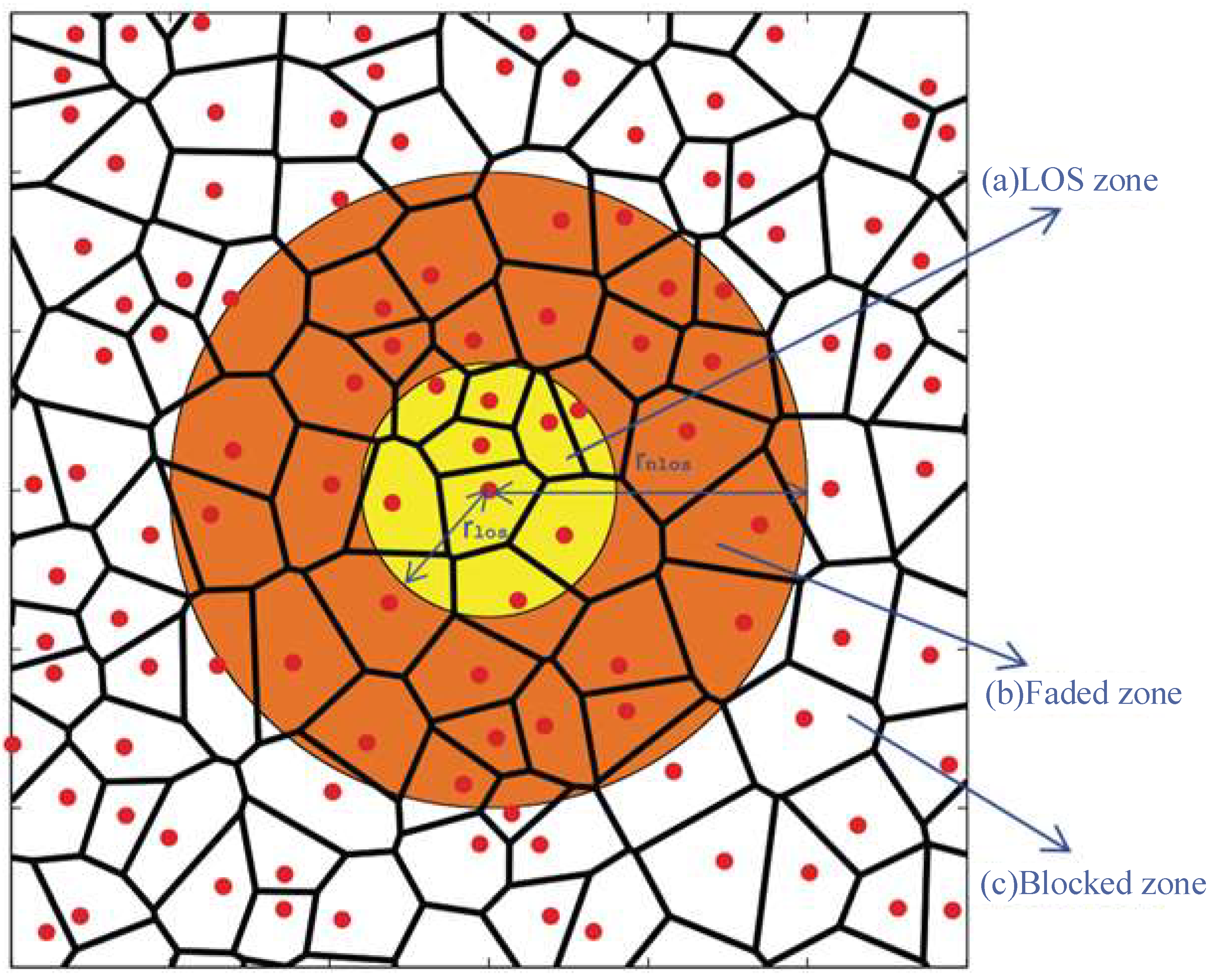
Figure 1 shows a typical network of 5G [4]. As illustrated via the red dots in the Figure, this network has some BSs (Base Stations) surrounded by a polygon cell, using Y_j to symbolize the j^th base station and its position [4]. If the referenced BS is Y₀ and the coordinate system is selected, it is at the origin, i.e., Y₀ = 0. Other BSs of the network can be placed in a casual way. For example, applying some known positions of an existing network or synthesizing through one stochastic-geometry model can locate these BSs. In the following parts, when having to specify the distribution of the BSs, the authors assumed that they were from a Uniform Clustering Process (UCP) of the intensity λ_bs. In it, every BS is around one exclusion zone with a radius of r_min.

Due to the underground roots, the researching work over root system is facing a very huge challenge. For the convenience of conducting more academic research on plants’ root, this article especially focuses on review of the study methods of plants’ root system. This paper consists of four sections: (1) Section 1, (2) Section 2, (3) Section 3, and (4) Section 4. In this paper, through the comparison of various research methods, we try to give a more accurate and feasible suggestion algorithm for root research. In the following parts of Section 1, the authors made prospects for the development and trends of plants system by reviewing them.

1.1. Traditional Research Methods on Plants Root

For a long time, people have studied the above-ground parts of plants far more than the underground root parts. The main reason is that plants’ roots are usually underground. We cannot directly observe or measure them, so plants’ roots are also called the “hidden half”. Plants’ root growth is complex, affected not only by temperature, water, soil fertility, and other environmental conditions, but also related to the growing stage of plants. It is precisely why some scholars point out that our understanding of the world under our feet is poorer than our knowledge of the universe [5], which also proves that root research is vital. Despite these, there are some traditional methods to research plants’ roots, such as digging method, drilling algorithm, container way, etc. In the following part below, we would like to describe what the process of these ways is, analyze, and compare their advantages and disadvantages.

There are two main observation methods for 3D (three-dimensional) study on plant roots under an underground soil environment: one is destructive, and another is non-destructive [6]. The following parts shown in

Table 1. Comparisons of Destructive methods.

Destructive Methods	Advantage	Disadvantage
Digging Method	direct measurement	time-consuming and laborious
Soil drilling Method	relatively easy and usual	harmful to the soil

list some comparisons of them.

Firstly, Table 1 above shows that the destructive methods are relatively easy and effective in achieving high throughput. Because of the high-throughput merit, these techniques are usually significant in large-scale genetic analysis and QTL (Quantitative Trait Locus) research. However, these ways are harmful to the root system and hardly analyze phenotypic traits.

Secondly, as for the non-destructive solutions, those non-destructive ways are used in large-scale non-destructive research, which can also be better in the research area of the large-scale genetic analysis, genetic analysis, and QTL research. There are some traditionally non-destructive detection methods shown in Figure 2 [5,6].

Table 2. Comparisons of non-destructive methods.

Destructive Methods	Advantage	Disadvantage
Internal growth Method	Direct measurement	Root growth limitation affected by the shape to some extent
Container Method	Root integrity	Root growth limitation affected by the shape to some extent
Isotope Probing Method	High detection accuracy	Uncertain effects of Isotope Probing
Soilless Cultivation Method	Free growth of roots	Dependent on the culture fluids to some extent
Mesh bag Method	Free growth of roots	Vulnerable to the environment
Minirhizotron Method	Relatively easy and usual	Root growth limitation affected by the shape to some extent

below shows that there are also a few high-throughput phenotypic methods in non-destructive technologies, so the QTL and the large-scale genetic analysis can apply them. Nevertheless, the results of these research techniques are usually based on ideal conditions and can not meet the actual soil environment.

Above all, although researching root morphological parameters is beneficial to learning about the condition of plants, there are not so many research results because of limited research conditions. With the development of modern science [7], some helpful research was studied and let the study of plants root be more in-depth. Furthermore, in the new century, there are some much more accurate methods that can explore plants’ roots via plant root physiological characteristics. Hence, more and more modern intelligent ways can detect and monitor plants’ roots to make more scientific decisions than before [8].

1.2. Modern Research Methods on Plants’ Roots

Conventional study methods on plant roots usually may have some errors due to unideal methods, even demolishing the original appearance of the plant roots. Therefore, most of those technologies cannot carefully and exactly obtain all the information about plants’ roots under no harmful conditions, especially some 3D messages on the roots’ structure and detailed distribution [9]. Within several years, in order to study both the 3D geomorphologic statistical distribution and conformation of the roots which are all located underground, some researchers investigated and probed the root systems’ 3D factors by applying many imaging techniques [10], including CCD Cameras, PET, X-rays and CT [11], etc. They all made outstanding donations and great contributions on how to use these plant roots to restore the ecologic balance.

Reconstruction of 3D pictures using images or the scheme of videos can furnish some beneficial knowledge, such as the distances and forms of 3D targets. Complete imaging can contrive the 3D show system with a diffraction grating and a lens array. Looking at the current technologies, some researchers would reconstruct the 3D images optically via the 2D (two-dimensional) usual show and add the lens array. We list some imaging ways below.

1.2.1. CCD (Charge-Coupled Device) Cameras Method

As shown in Figure 3, CCD is a device for the movement of electrical charge, usually from within the device to an area where the charge can be manipulated, for example conversion into a digital value. On this way, the system uses an array of the micro-lens to construct the 3D object and a CCD camera to mark the information. So, we can apply the special computer for picking up the key pixels to construct a 3D picture.

To study more, some root systems [12] have already used the CCD camera owing to the accurate locating responsibility. Virtually, other scientists applied the “Hybrid Algorithm,” which is the digital imaging techniques mixed with the roots’ fractal technology to acquire the 3D pictures from those root systems [13] as well. The authors put the root pictures obtained by taking rotationally into a software system programmed by themselves to reconstruct its 3D structure [14].

1.2.2. PET (Positron Emission Computed Tomography) Method

PET uses small amounts of radioactive materials called radiotracers, a special camera, and a computer to help evaluate your organ and tissue functions. By identifying body changes at the cellular level, PET may detect the early onset of disease before it is evident on other imaging tests.

In order to conduct research on the imaging of plant roots, many PET scanners were established. These PET scanners almost apply 3D imaging technology. For examples, the researcher applied a PETIS system which has some modules of the flat detector at a very big area for obtaining plants’ projection pictures in Japan. As well as in the lab of scientist Jefferson, he has developed the PhytoPET [16]. In Germany, to give the pictures of the tomographic PET, a research group [17] built the PET scanner for the partial ring with eight detector parts. Then the full circle PET scanners for plants were constructed by Brookhaven [18] and Budassi [19]. These many endeavors and tries show that there is more and more interest in the PET research on plant roots recently. The PET/CT scanner was developed as a combination of a Siemens Somatom AR.SP spiral CT [18] and a partial-ring, rotating ECAT ART PET scanner [19]. All components are mounted on a common rotational support within a single gantry [20]. The researchers provide a 15 cm-diameter trans-axial field of view (FOV) for dynamic tomographic imaging of small plants.

1.2.3. X-ray CT (X-ray Computed Tomography)

As an X-ray imaging processing technology, the operating process of CT includes the following four steps: (1) CT uses the X-ray beam to scan some examination areas; (2) the detector could receive and transmit the X-ray, and the X-ray is converted into light that is visible to us; (3) visible light intends to be an electrical signal by the photoelectric converter [21]; (4) applying an analog/digital module, the signals are going to be input into the computer for further processing in the mode of the discrete digital signals.

Hartmann first applied CT to survey the 3D pictures from the roots which are planted in some PVC pipe. Author utilized the scanning of the CT methods for measurement on some pictures of the roots which are planted inside a container [22]. The data scanned via CT could be utilized to precisely measure the factors, including average length of the roots, whole volume, the surface, average diameter, peak diameter, erect deepness, etc. The article [23] made an overview of how to reconstruct the root system by the usage of CT scanning. The paper [24] researched and built a 3D system of the plant roots with the technique on images process via CT scan. In addition, by scanning the circle multi-slice CT [25,26], a researcher can precisely and non-destructively obtain a proper morphology of the 3D plant roots system. Other results of the papers [27,28,29] have demonstrated that to investigate the roots structure in 3D model, CT is a pretty good way to accomplish this efficiently.

1.2.4. MRI (Magnetic Resonance Imaging)

MRI is a medical imaging technique used in radiology to form pictures of the anatomy and the physiological processes of the body [30]. MRI scanners use strong magnetic fields, magnetic field gradients, and radio waves to generate images of the organs in the body [31].

1.3. Some Cutting-Edge Techniques

1.3.1. The Carbon Dynamics Method

Scientists established an easy way which put one wide-view scanner underground to keep monitoring the rhizosphere [32]. This system with an optical scanner can help researchers to analyze the data of the root images and supervisory control constantly via fixing the place of the scanners and automatic capture. Their expert monitoring system has undertaken some experiments in their lab. Furthermore, in the real environment, a system over the CO₂ measurement was set up. Some pictures with high resolution can be achieved by the monitoring system, concluding a lot of possibilities on continuously analyzing the live-dead-decomposition roots dynamic.

1.3.2. The Root-Microbe Communication Method

Currently, more and more scientists [33] are spotlighting the influences the microbial communities can have on the plants’ health and development. Those impacts on plants include changes in quality and amount of area, the timing of the significant developing periods, and permissiveness from the abiotic or biotic pressures. It is obvious that learning these effects which can donate to the plant-beneficial roots microbiome may prove advantageous. Metzner, R. [34] conducted the research on some recent knowledge over the establishment and sustainment of the microbial communities which are relative of the roots and plants-microbe interactions with the special accent over the effects of those microbe interactions on a figure of the microbial communities on the top of the roots. In addition, he and his colleagues also studied the possibility for the roots’ microbiome modification to profit agriculture industry and production of the food.

1.3.3. The Root Exudates on Rhizosphere Water Dynamics Method

The nutritional components and the most water which are vital for plants go through the rhizosphere that is a slender area of the soil at the merging zone among the soil and roots. The chemistry components released via the plants’ roots can change some fluid attributes, such as viscousness, water phase, potential effects on stress tolerance, and plants’ productivity [34].

1.3.4. Diameter Classification Method of Fine Root

To make it easy on sorting process, Azzari, G. applied the diameter of the plants roots as an agency. This way also can evade the problem of having to designate the roots to a specific root order. This method offers a totally novel and reasonable way to advance the plant roots order approach. Nevertheless, different plants have different morphology of their roots. Therefore, it is the better way that we could, respectively, build the relationship among the diameter and roots order according to separate plants in the real environments [35]. Consequently, this relationship module can be used to offer the fundamental knowledge of how to predict the roots’ factors more precisely.

1.4. Current Shortcomings and Difficulties

The study of plant root morphological parameters has attracted wide attention in the study of ecosystem and climate change [36]. The morphological parameters of plants’ roots mainly include topological structure, length, root length and density, root torsion degree, root growth angle, root tip number, etc. Due to underground growing and complicated distribution, gathering the information of a plant’s roots is very hard [37].

Recording the features mentioned above is almost always conducted by hand, so we should find a much better solution to promote assessing factors of accuracy and speed via utilizing the visible picturing. A visible imaging of the plants’ phenotyping is an easier way, while those pictures are just able to offer the plants’ physiological message of the plants phenotyping. Consequently, when the visible pictures are processed to achieve the 3D phenotypic message such as the leaves’ number, the leaves’ area, the biomass, etc., it still has the challenge of how to deal with the special overlap of the adjacent leaves within an image segment. In addition to this problem, to apply it well, there are other questions and limitations below: (I) the leaves and their background are too hard to distinguish no matter what the color and brightness are concerned; (II) the clearance of the shadow which is from the canopy; (III) an image construction once some insects and soil are removed from the leaf; and (IV) the affection of light over using the picture processing automatically. The elements above severely influence the usage of the visible picturing to plants phenotyping in the field, so they must be dealt with via the other methods and technologies.

The methods mentioned in the last part almost have their own advantages and disadvantages as well, and every way can be improved in performance in terms of the recognition rate and dealing speed using mixed techniques. In this article, we proposed a high-throughput method and process for plant three-dimensional root phenotype and reconstruction based on X-ray CT technology. Beginning with a high-throughput transmission of the root phenotype in addition to utilizing the imaging technique to extract the root characteristics, this study furthermore adopts a moving cube algorithm to reconstruct the three-dimensional root. In conclusion, the experimental results show that the presented method in this paper works well. It may provide an efficient idea for the detection of the root phenotype.

The structure of this paper is as follows: Section 1 reviews some solutions for root phenotype; Section 2 gives Proposed System Model and Theory; Section 3 shows the results and their analysis; Section 4 concludes this article lastly.

2. Proposed System Model and Theory

As shown in Figure 4 below, the Proposed System Model in the article has four stages: CT imaging, high flux image transmission, image preprocessing, and three-dimensional root reconstruction. The following parts illustrate these steps, especially for the high flux image transmission and three-dimensional root reconstruction in detail.

2.1. Model of the CT Imaging

X-ray CT imaging can generate a cross-sectional image of the root soil, and there is somewhat X-ray fading due to penetrating the object. According to Lambert’s law in physics, when a monochromatic harness passes through an object with uniform density, the harnessed energy weakens because of an interaction between the harnessed energy and the material atoms, and the weakening degree depends on the material thickness, absorption coefficient, and composition [38]; the following equation can express it:

$$I=I_0{e}^{-\mu d}$$

(1)

In Equation (1), I₀ is the intensity of the incident X-ray (i.e., the transmitting energy); the index of I is the intensity after transmission (i.e., the receiving one) that was passing through a uniform density object; μ Is the linear coefficient of the substance to the wavelength; d is the path length through a uniform density object, and e is the natural logarithmic base. As seen from the equation, because the value of μ depends upon X-ray energy, atomic coefficient, and density of matter $\rho$ (as shown in Figure 5), there is a much larger D or μ and much smaller I₀ the larger the fading of X-rays is. In it, D represents a uniform distance of parameter d.

Assuming that the object is composed of several segments with an equal length, each part has a distance of D, and D is small enough. Otherwise, the density and the fading coefficient of every segment are consistent. If the incident intensity of the first segment of this X-ray with a length of D is I₀, then the transmitted X-ray intensity I₁ of the first section can be obtained according to the Equation (1). So, as for segment n:

$$I_n=I_0{e}^{-\left({\mu }_{1}d+{\mu }_{2}d+\cdots +{\mu }_{n}d\right)}$$

(2)

Transform Equation (2) using algorithm computation to obtain Equation (3) below:

$${\mu }_1+{\mu }_2+\cdots +{\mu }_n=\frac{1}{d}\ln \frac{I_0}{I_n}$$

(3)

Therefore, when D, I₀, and I₁ are known, the calculation of μ value needs to establish equations of projections in multiple directions. In Equation (3), μ is the attenuation coefficient of X-rays [39]. During X-ray tomography, utilizing X-ray can scan voxels in every fault and simulate to generate a CT value. Authors may regard this small space as a cube, and the 3D image after X-ray CT scanning (as shown in Figure 6 below) is the tomographic image data obtained by X-ray CT imaging.

2.2. Model of the High-Throughput Image Transmission

Figure 7 illustrates the model of the high-throughput image transmission proposed in this research. The model includes an imaging port, a reconstruction end, and the 5G linking channel.

As shown from the figure above, to meet the current requirement of the transmitting speed for high throughput in the 5G network, the authors chose a 5G linking channel simplified from Figure 1 as the experimental transmission method (shown in Figure 8 below) [40]. Figure 8 below shows a typical network presented and applied in the author’s previous research.

Since there are some distance-loss, shadowing-loss, and multi-path fading in this network, more sending powers are required via lots of VCs (Virtual Cells) while they exchange messages with central ports directly. The multi-hop networks could decline this problem.

Those signals of the net should be relayed via these VCs. In other words, a number of VCs can communicate smoothly with central ports in whatever downlink or uplink transmissions of the data.

The equation 4 below denotes sending power. The assumption in this system is that there are perfectly rake combining [41] and TPC (Transmit Power Control) [42] work well to value accurately sending powers. Secondly, the Rayleigh fading channel [43] is assumed as L-path, and none of the diversity is utilized in the multi hop relay network, so a transmit power P_t(i) from port #i is expressed by

$$P_t\left(i\right)=\frac{P_{req}}{d_{i,j}^{-\alpha }{10}^{-\frac{{\eta }_{i,j}}{10}}{{\displaystyle \sum }}_{l=0}^{L-1}{\left|{\xi }_{i,j}\left(l\right)\right|}^2}$$

(4)

where P_t is the transmitting image, and P_req denotes the receiving image. There are some definitions, including the shadowing loss η_i,j (in dB), l-th path complex path gain ξ_i,j, path-loss exponent α, and the distance d_i,j, etc. If we propose that the ensemble average operation is E[*], then we can obtain $E\left[{\left|{\xi }_{i,j}\right|}^2\right]=1/L$; independent complex Gaussian variables with zero-mean are {ξ_i,j}.

Therefore, the mobile terminal transmitting power P_t(0) is expressed as

$$P_t\left(0\right)=\frac{P_{req}}{d_{0,1}^{-\alpha }{10}^{-\frac{{\eta }_{0,1}}{10}}{{\displaystyle \sum }}_{l=0}^{L-1}{\left|{\xi }_{0,1}\left(l\right)\right|}^2}$$

(5)

2.3. Model of the Image Preprocessing

2.3.1. Image-Denoising

Image denoising is a vital step for image pre-processing, and the results of image denoising will directly affect the quality of mid-term segmentation. As for image-denoising methods, the author considers three various ways: Butterworth low-pass filter, mean low-pass filtering, and median filtering. However, during the simulation, the authors found that the mean filter and the Butterworth filter are equivalent to the low-pass filter, which tends to blur the image and is powerless to deal with salt and pepper noise filtered by the median filter well. Therefore, in the face of the root CT image with pepper and salt noise studied in this paper, the authors finally selected the median filter for image denoising. This part performed the simulation on the image denoising using a simulating tool of MATLAB and the same way for the rest sections.

As shown in Figure 9 below, this paper chose the median filter to filter the noise. Its basic principle is to replace the value of a pixel in the image using the median of each point in its surrounding neighborhood [44]. This filter (as shown in Figure 9a) can filter the noise and protect the image edge to the specific case of soil CT tomographic image. According to the actual condition in this research and to better adapt to the in situ root CT image (as shown in Figure 9b), the authors chose a 9 × 9 template median filtering. The center value of the template matrix is the median of eight surrounding points in its circle, and the total energy of the image template signal remains unchanged to obtain the filtered image (as shown in Figure 9c).

As found in Figure 9, by comparing the original and filter image, utilizing this selected nine × nine template median filtering could remove most of the noise in the original image and better keep the picture edge at most.

2.3.2. Image Segmentation

After removing noise and highlighting root features through image-denoising, threshold segmentation is a reasonable method to extract root features. The parameter used for threshold segmentation of root CT image in this paper is 225, the same as the median filter in image denoising in the previous section. This selection for the threshold means the pixels valued less than the threshold are white, and others with more than the threshold are black or background to split the image in the image segmentation.

As shown in Figure 10 above, applying the filtered denoised image and its histogram of CT sectional image can obtain the threshold range of root feature; then, using threshold segmentation can achieve the segmented CT sectional image with root feature.

2.3.3. Preprocessing for Reconstruction

Due to these problems caused by the complex structure of the soil medium, such influencing factors mentioned above default as root characteristics during segmentation. Therefore, it needs marking and highlighting the root feature via combining the filtered image as shown in Figure 11 below.

By analyzing the actual situation and comparing the original image with the image after threshold segmentation we find that there may be uneven density distribution in the soil, resulting in different imaging gray levels, or the edge of the plant is consistent with the gray levels of the root system. Furthermore, even if there is only a little air and water in the soil, it causes the same problem above. Consequently, this preprocess is significant that combines the filtered image to mark or highlight the root feature in advance.

2.4. Model of the Three-Dimensional Root Reconstruction

The study adopts a moving cube algorithm to reconstruct the three-dimensional root. The main idea of this method in the field of reconstruction is as follows four steps:

• It firstly regards a two-dimensional fault slice sequence as a three-dimensional data area;
• It processes each voxel and compares the values of eight vertices of each voxel with the given threshold extracted from the data area, secondly;
• It then determines the position of the isosurface, obtains the voxel isosurface, and calculates relevant parameters;
• Finally, it fits the patches and reconstructs the data from each voxel into the isosurface of the original root system.

Voxel used in the algorithm is the smallest unit of data in three-dimensional space. As shown in Figure 12a below, the space coordinates of eight vertices defining each voxel are $(a,b,c)$, $(a+1,b,c)$, $(a,b+1,c)$, $(a+1,b+1,c)$, $(a,b,c+1)$, $(a+1,b,c+1)$, $(a,b+1,c+1)$, $(a+1,b+1,c+1)$, respectively. Figure 12b also illustrates the tomographic slice voxel sequence in its right one.

As shown in Figure 12 above, the sampling value corresponding to point P in this image is the cubic linear interpolation result of eight voxel values of the voxel boundary. Supposing that the sampling spacing in X, Y, and Z directions is $\mathsf{\Delta }x$, $\mathsf{\Delta }y$, and $\mathsf{\Delta }z$, as well as eight fixed-point values in voxel are $m_0(x_0,y_0,z_0)$, $m_1(x_0,y_0,z_1)$, $m_2(x_0,y_1,z_0)$, $m_3(x_0,y_1,z_1)$, $m_4(x_1,y_0,z_0)$, $m_5(x_1,y_0,z_1)$, $m_6(x_1,y_1,z_0)$, $m_7(x_1,y_1,z_1)$, then an interpolation definition of the point P is:

$$\begin{array}{l}p=\frac{x_1-x}{\mathsf{\Delta }x}\times \frac{y-y_0}{\mathsf{\Delta }y}\times \frac{z_1-z}{\mathsf{\Delta }z}\times m_0+\frac{x_1-x}{\mathsf{\Delta }x}\times \frac{y_1-y}{\mathsf{\Delta }y}\times \frac{z_1-z}{\mathsf{\Delta }z}\times m_1+\\ \begin{array}{cc}& \frac{x-x_0}{\mathsf{\Delta }x}\times \frac{y_1-y}{\mathsf{\Delta }y}\times \frac{z_1-z}{\mathsf{\Delta }z}\times m_2+\end{array}\frac{x-x_0}{\mathsf{\Delta }x}\times \frac{y-y_0}{\mathsf{\Delta }y}\times \frac{z_1-z}{\mathsf{\Delta }z}\times m_3+\\ \begin{array}{cc}& \frac{x_1-x}{\mathsf{\Delta }x}\times \frac{y-y_0}{\mathsf{\Delta }y}\times \frac{z-z_0}{\mathsf{\Delta }z}\times m_4+\frac{x_1-x}{\mathsf{\Delta }x}\times \frac{y_1-y}{\mathsf{\Delta }y}\times \frac{z-z_0}{\mathsf{\Delta }z}\times m_5+\end{array}\\ \begin{array}{cc}& \frac{x_1-x}{\mathsf{\Delta }x}\times \frac{y_1-y}{\mathsf{\Delta }y}\times \frac{z-z_0}{\mathsf{\Delta }z}\times m_6+\frac{x-x_0}{\mathsf{\Delta }x}\times \frac{y-y_0}{\mathsf{\Delta }y}\times \frac{z-z_0}{\mathsf{\Delta }z}\times m_7\end{array}\end{array}$$

(6)

After sorting:

$$p(x,y,z)=l_0+l_{1}x+l_{2}y+l_{3}z+l_{4}xy+l_{5}yz+l_{6}xz+l_{7}xyz$$

(7)

where $l_0~l_7$ is constant determined by $m_0~m_7$ based on Equations (6) and (7) above. Therefore, in the three-dimensional data space, the point set with the same value in the isosurface is $\{(x,y,z)|p(x,y,z)=c\}$, and c is a constant.

The three-dimensional visualization of root X-ray CT tomography volume data is a visualization of three-dimensional spatial data. The sectional image data of plant roots obtained by X-ray CT equipment are regular in three-dimensional spatial data fields after encapsulation. Regularly structured data are spatially discrete data logically organized into a three-dimensional array. Each element of these spatially discrete data possesses a logical relationship with the data of the three-dimensional array, and each voxel can have its row number, column number, and layer number. Figure 13 below shows the algorithm flow of a moving cube.

The moving cube algorithm can extract a series of isosurfaces from a three-dimensional data field. Figure 13. above illustrates the algorithm flow of the moving cube. In the process of this method, process the voxels in the data field one by one firstly, and classify the cubes intersecting with the isosurface secondly. Finally, calculate the intersection point between the isosurface and the cube edge by interpolation, based on the relative position between every vertex and the isosurface. It considers an isosurface the approximate representation. This isosurface is generated by connecting intersection points between an isosurface and the cube edges.

3. Results and Analysis

Because of pretty hierarchal and diverse scheme, the method of the root order is better than the root diameter method reviewed in Section 1.3.4 to reconstruct the plants’ root system. Nevertheless, the complexity of the root order method limits its applications. Currently, scientists have researched some solutions. One of these reasonable ways is to utilize the least number of those root orders as possible.

As seen from Figure 14, the method of five root orders has three main parts to distinguish the five growth processes of plant roots [45]. These three parts are a module for the experimental designs, a module of measurement on quantitative computing, and a module for results explanations. Figure 15 below gives the result for the method of five root orders.

The best design of the experiments should consider the different growth environments. Meanwhile, this process should also regard the planting environment, the plants’ growing structure, and the infrastructural handling. The module of the measurement on quantitative computing operates well under some cutting-edge technologies of picturing but requires a series of standard protocols during the experiments, including an accurate definition description of the processing regulation for raw data and the calibration of the picturing sensors, regarding the part of the best process for analyzing the plants’ phenotyping.

Figure 15 above illustrates the result for the method of five root orders. According to the method of the five root orders mentioned above, we can define and distinguish that the root orders from first- to fifth-order, respectively, denote five stages of the plants: Emergence, Full cover, Anthesis, Maturity, and Harvest. As found from the figure, those solid profiles with the different colors represent the functions of the probability distribution structured by diameters, respectively, corresponding to these first through fifth orders of the root of plants. The cross values of these probability functions distribution curves of the diameter of the two nearly root orders are only the threshold of this diameter interval. Regarding the diameters corresponding to the cross units of the probability distribution lines upon these five orders for the roots of plants as segment threshold values of next near order roots, these thresholds for those diameters from first- to fifth-root orders are 0.478 mm, 0.732 mm, 1.062 mm, 1.453 mm, and more than 1.453 mm, respectively.

After sorting and distinguishing first- to fifth-root orders of the roots for plants, as long as the spatial position of a corner of the three-dimensional grid and the serial number of a given data point, using the distance corresponding to the grid spacing can calculate the spatial position of the root profile, then through the measurement of three-dimensional parameters may obtain the root configuration data such as root surface area and volume for further refining the three-dimensional data of plant roots. Figure 16 shows the visualization process model of the sectional image, and Figure 17 illustrates the three-dimensional visual simulation of the root system.

Measuring and calculating the three-dimensional parameters of the root system, using the moving cube algorithm and applying a drawing tool for figuring the three-dimension image (named OPENSIMROOT), can carry out a three-dimensional visual reconstruction of the obtained CT image sequence. Figure 17 above is a three-dimensional visual simulation reconstruction model of the root system.

Figure 18 below shows the front-view, left-view, and right-view of the root reconstruction system rotating and transforming the spatial coordinate axis.

From the two figures above, using the proposed method can transmit the root image in high throughput well due to little noise and the detailed structure of the root.

4. Conclusions

This paper proposed a high-throughput method for plant three-dimensional root reconstruction based on X-ray CT three-dimensional root tomography technology to boost the research on the 3D reconstruction of root phenotyping of plants. The article took advantage of the characteristics of fast data transmission speed and large throughput of 5G wireless transmission links which can effectively reduce the time of image data transmission between the imaging terminal and the lower computer in the image transmission.

In this report, the presented algorithm can carry out effective high-throughput transmitting for the root reconstruction of plants first; secondly, the article applied image filtering and segmentation techniques suitable for the research conditions to study three-dimensional root phenotype; finally, this article demonstrated the operation of three-dimensional reconstruction of the roots system by calculating the three-dimensional parameters of the root system and using the moving cube algorithm.

The simulation results show that the proposed method based on X-ray CT in this paper works well, which can give new ideas to research plant root phenotype in the future study.