Minimally Persistent Graph Generation and Formation Control for Multi-Robot Systems under Sensing Constraints

Abstract

This paper presents a minimally persistent graph generation and formation control strategy for multi-robot systems with sensing constraints. Specifically, each robot has a limited field of view (FOV) and range sensing capability. To tackle this problem, one needs to construct an appropriate interaction topology, namely assign neighbors to each robot such that all their sensing constraints are satisfied. In addition, as a stringent yet reasonable guarantee for the visual constraints, it is also required that the prescribed neighbors always stay within its visual field during the formation evolution. To this end, given a set of feasible initial positions, we first present a depth-first-search (DFS)-based algorithm to generate a minimally persistent graph, which encodes the sensing constraints via its directed edges. Then, based on the resultant graph, by invoking the gradient-based control technique and control barrier function (CBF), we propose a class of distributed formation control laws, rendering not only the convergence to the desired formation but also the satisfaction of sensing constraints. Simulation and experimental results are presented to verify the effectiveness of the proposed approach.

1. Introduction

Multi-robot formation control has received much attention in recent years due to its many applications in various fields, such as collective transportation, exploration, and surveillance [1]. Diverse formation control methods have been reported, including a leader–follower scheme [2], behavior-based technique [3], virtual structure [4], graph theory-based method [5], and many others [6,7,8].

In consideration of the vulnerability of intercommunication to cyber-attacks when securing relative states, the manner of on-board sensing is more preferred in practical implementations. From the perspective of sensing capabilities, the so-called vision-based formation control framework has been widely reported due to its low cost and increasing measurement accuracy [9,10,11]. However, it is worth noting that these on-board sensors such as cameras always suffer from limited field of view and visual range constraints which inevitably affect robots’ motions [12]. Therefore, it is desirable to develop new feasible algorithms to overcome these problems.

Early efforts have been devoted to designing proper control laws to cope with sensing constraints. In [12], a gradient descent-like control algorithm is proposed to form a “compatible formation”, in which each robot is equipped with a fish-eye camera that only provides limited FOV and range measurements. By restricting each quadrotor to stay within the visible region of others, the sensing connections can be maintained, leading asymptotic convergence to the desired formation. However, the algorithm requires that any pair robots have to observe each other all the time, which implies that the underlying graph is complete. Other works addressing sensing constraints can be found in [13,14,15,16]. All these methods proposed therein are valid under the condition that the underlying graph has to be known a priori.

It is known that graph rigidity theory plays a key role in formation control of multi-robot systems [17]. In recent years, several works have concentrated on constructing rigid graphs. In [18], the pebble game algorithm is presented to generate a minimally rigid graph in the plane. A theoretical framework is provided to analyze the persistence property of formation shapes [19]. Moreover, the Henneberg construction is also extended to the directed version to generate the minimally persistent graph therein. Even though undirected minimally rigid graphs can be constructed by Henneberg construction, in general one cannot always obtain a minimally persistent graph via directed Henneberg construction operations on some particular types of seed graphs. Later, the directed Henneberg construction is further extended by introducing the edge reversal operation [20]. It is worth noting that these results provide us with construction principles from the pure graph point of view without taking the physical constraints such as limited field of view and distance sensing range into account. In [21], a Delaunay triangulation-based algorithm is presented to generate a relation-invariable persistent formation, in which edge relations cannot be changed. With the aim of minimizing communication complexity and reducing energy consumption, a rigidity matrix-based approach is proposed to construct min-weighted rigid and persistent graphs [22]. However, this approach requires the calculation of the rank of rigidity matrix at each step, leading to high computational complexity. Moreover, construction of formations with range constraints is considered in a rigidity matrix-based method [22]. In the situation where the robots have limited sensing range, the pebble game algorithm is extended to grow minimally persistent formations [23]. In [24,25], the limited communication range constraint is overcome by appropriately integrating rigid subgraphs built by each node locally. However, note that all the above-mentioned methods would lose effectiveness if robots were encountered with both FOV and sensing range constraints concurrently.

Partially inspired by [23], the objective of this paper is first to propose an algorithm to generate a minimally persistent graph representing robots’ sensing relationships under both limited FOV and range constraints, and then design distributed admissible control laws to achieve desired formation. To be specific, based on the pebble game algorithm, we present a DFS-based constructing method incorporating elaborated principles of degree of freedom (DOF) transfer, with which the sensing constraints can be always satisfied during graph generation. To the best of our knowledge, it is the first algorithm that considers both the visual range and FOV constraints when constructing minimally persistent graphs. Furthermore, to solve the constrained formation control problem, we propose an integrated control framework by invoking gradient descent control technique and CBF. To activate the CBF, the forward invariance of the safe set needs to be maintained. As a consequence, the initial configuration of the robots must be confined in the safe set, which requires the global intervention in most references such as [26,27,28], while by employing our method, the generated graphs are naturally compatible with the constraints of CBF employed in formation control. With the proposed control law, the implicit connectivity in terms of the sensing topology are maintained along with the convergence to the desired formation.

The rest of this paper is organized as follows. Section 2 introduces the concepts of rigid and persistent graph, CBF, and the pebble game algorithm as well as the problem statement. In Section 3, we present the construction algorithm yielding a minimally persistent formation with sensing constraints, followed by the corresponding distributed control framework. Section 4 shows simulation and experimental results. Section 5 gives the conclusion.

2. Preliminaries and Problem Statement

This section first reviews some basic concepts that will be used throughout this paper and then addresses the problem to be solved.

2.1. Rigid and Persistent Graph

A graph $G=(V,E)$ is used to represent the interaction relationship of a group of n robots, where $V=\{1,2,\dots ,n\}$ is the vertex set and $E=\left\{\right(i,j),i,j\in V,i\ne j\}$ is the edge set. Let $p_i\left(t\right)\in {\mathbb{R}}^2$ denote the position of vertex i. For a desired configuration $p^{*}\in {\mathbb{R}}^{2n}$ defined by $p^{*}={[p_1^{*\mathrm{T}},\dots ,p_n^{*\mathrm{T}}]}^{\mathrm{T}}$, an edge-consistent trajectory is defined as one such that $\forall (i,j)\in E$, $\parallel p_i\left(t\right)-p_j\left(t\right)\parallel = \parallel p_i^{*}\left(t\right)-p_j^{*}\left(t\right)\parallel , t>0$. A rigid trajectory is defined in such a manner that $\forall (i,j)\in V\times V,\parallel p_i\left(t\right)-p_j\left(t\right)\parallel = \parallel p_i^{*}\left(t\right)-p_j^{*}\left(t\right)\parallel , t>0$. If all edge-consistent trajectories are rigid trajectories, the graph $G=(V,E)$ is a rigid graph. Laman gives the necessary and sufficient condition for a graph being minimally rigid in two-dimensional space.

Lemma 1 

(Laman’s Theorem [29]). A graph $G=(V,E)$ is minimally rigid if and only if it has $2n-3$ edges and no induced subgraph $G^{\prime }=(V^{\prime },E^{\prime })$ has more than $2n^{\prime }-3$ edges.

A persistent graph can be obtained generally by adding a direction to every edge of a rigid graph. The directed edge $(i,j)$ implies that vertex i can receive information from vertex j, but not vice versa. For a vertex i in a persistent graph $G=(V,E)$, $N_i=\{j:(i,j)\in E\}$ denotes the neighbor set of i. The out-degree of vertex i is defined as the number of edges leaving from i. A minimally persistent graph is a persistent graph whose edges cannot be removed without losing persistence [19].

Lemma 2 

([30]). A graph is minimally persistent if and only if it is minimally rigid and no vertex has an out-degree larger than 2.

2.2. Control Barrier Function

Control barrier function proposed by [31,32] has been widely used in safety critical systems. Following [33,34], we give the brief introduction to CBF. Consider a nonlinear affine control system given by

$$\dot{x}=f\left(x\right)+g\left(x\right)u,$$

(1)

where f and g are locally Lipschitz, $x\in {\mathbb{R}}^n$ and $u\in U\subset {\mathbb{R}}^m$ (U denotes the control constraint set).

Assume that $h\left(x\right):{\mathbb{R}}^n\to \mathbb{R}$ is a continuously differentiable function. The safe set $\mathcal{C}$ is defined as

$$\begin{array}{cc}\hfill \mathcal{C}& =\left\{x\in {\mathbb{R}}^n:h\left(x\right)\ge 0\right\},\hfill \\ \hfill \partial \mathcal{C}& =\left\{x\in {\mathbb{R}}^n:h\left(x\right)=0\right\},\hfill \\ \hfill Int\left(\mathcal{C}\right)& =\left\{x\in {\mathbb{R}}^n:h\left(x\right)>0\right\},\hfill \end{array}$$

(2)

where $\partial \mathcal{C}$ and $Int\left(\mathcal{C}\right)$ denote the boundary and interior of $\mathcal{C}$, respectively.

A continuous function $\kappa :(-b,a)\to (-\infty ,\infty )$ is said to belong to extended class $\mathcal{K}$ if it is strictly increasing and $\kappa \left(0\right)=0$. Given a safe set $\mathcal{C}$ defined in (2) for a continuously differentiable function $h\left(x\right):{\mathbb{R}}^n\to \mathbb{R}$, the function $h\left(x\right)$ is called a CBF, if there exists an extended class $\mathcal{K}$ function $\kappa$ such that

$$\underset{u\in U}{sup}\left\{\frac{\partial h\left(x\right)}{\partial t}+L_{f}h\left(x\right)+L_{g}h\left(x\right)u+\kappa \left(h\left(x\right)\right)\right\}\ge 0$$

(3)

holds for any $x\in \mathcal{C}$.

Given a CBF $h\left(x\right)$, for all $x\in \mathcal{C}$ define the set

$$K=\left\{u\in U:\frac{\partial h\left(x\right)}{\partial t}+L_{f}h\left(x\right)+L_{g}h\left(x\right)u+\kappa \left(h\left(x\right)\right)\ge 0\right\},$$

(4)

such that any Lipschitz continuous controller $u\in K$ will keep the system safe.

2.3. The Pebble Game Algorithm

The pebble game algorithm proposed in [18] is used to generate minimally rigid graphs in a two-dimensional space. In the algorithm, each vertex is assigned two pebbles representing the vertex’s DOF. These two pebbles are used to cover any two edges incident to that vertex. The algorithm is initialized with an empty graph and grown by adding one directed edge at each step. The tail of the edge is assigned to the vertex with a covered pebble. If all edges in the graph are covered, it is called a pebble covering. When inserting new edges, one needs to search for free pebbles in the existing directed graph. Once a free pebble is found at one vertex, a sequence of edge reversing operations is implemented to free up a pebble of the endpoint to cover a new edge. If there exists a pebble covering when a new edge is quadrupled (i.e., operation of adding three additional edges between the same pair of endpoints), it implies that no induced subgraph $G^{\prime }=(V^{\prime },E^{\prime })$ has more than $2n^{\prime }-3$ edges, namely the second half of Laman’s theorem is satisfied. In this situation, we say that this newly added edge is independent of the pre-existing edges collected in the set $\widehat{E}$ and can be added to the graph. Therefore, if the graph contains $2n-3$ edges, the first half of Laman’s theorem is thus satisfied, yielding a minimally rigid graph. Interested readers are referred to [18] for further details.

Lemma 3 

([18]). A new edge e is independent of $\widehat{E}$ if and only if there exists a pebble covering when e is quadrupled.

2.4. Problem Formulation

In this paper, we consider a group of robots whose dynamic are given by

$$\begin{array}{ccc}\hfill {\dot{q}}_i\left(t\right)& =u_i\left(t\right),\hfill & \\ \hfill {\dot{\theta }}_i\left(t\right)& ={\omega }_i\left(t\right),\hfill \end{array}$$

(5)

where $q_i={[x_i,y_i]}^{\mathrm{T}}\in R^2$ and ${\theta }_i$ represent the position and the yaw angle of the ith robot, respectively. $u_i$ and ${\omega }_i$ denote the control inputs. For simplicity, the variable t is omitted unless otherwise stated.

Consider a group of planar robots modeled by (5). Each robot is equipped with a camera with limited FOV and finite sensing range R. It is assumed that the camera is fixed at the head of the robot and its yaw angle can be controlled independently. The objective is to construct an interaction topology satisfying above-mentioned sensing constraints, and utilize the measurements obtained by the front camera to achieve the desired formation as well as maintain the connectivity of the underlying sensing topology. This problem can be found in a scenario where a group of robots undertake the exploration or navigation task in GPS and communication partially denied environment.

3. Main Results

This section begins with the introduction of several basic concepts. Then a modified version, named as FOV pebble game, is presented under FOV and limited sensing range constraints. Based on the resultant persistent graph, we then propose a distributed control framework by invoking CBF and gradient-based control technique.

To facilitate the following discussions, we first give a couple of definitions.

3.1. Definitions

Akin to persistent feasibility in [23], the definition of minimally FOV persistent graph is given as follows.

Definition 1. 

Given an angle α and a positive scalar R representing the field of view and sensing range, a graph G is called a minimally FOV persistent graph if and only if it is a minimally persistent graph and the internal angles formed by two leaving edges are no more than α, and the length of each edge does not exceed R.

Remark 1. 

Note that a minimally FOV persistent graph must be a minimally persistent graph, but not vice versa. From Lemma 2, except for the vertices with out-degree two, each vertex has zero or one neighbor. Hence, these vertices intrinsically satisfy the angle constraints. Figure 1 shows the difference between a general minimally persistent graph and a minimally FOV persistent graph.

Now, we give the definitions of transferable pebble and fixed pebble.

Definition 2. 

If a pebble at a vertex can be transferred to another vertex by reversing the directed edge (or directed path) without violating the sensing constraints, it is called a transferable pebble. Otherwise, it is called a fixed pebble.

Remark 2. 

Note that “transfer" here does not mean moving a pebble from one vertex to another. By reversing the edge $(i,j)$, one can free up a pebble at vertex i, and thus use a pebble of j to cover the edge instead. In the pebble game algorithm, since all pebbles can be freely transferred, they are all transferable pebbles.

When searching for pebbles, to satisfy the FOV constraints, one must determine whether the free pebble is transferable. Once a transferable pebble is found, it succeeds to free up a pebble to cover a new edge by edge reversing operations. If a pebble is identified as a fixed pebble, it will be recorded. The goal is to find transferable pebbles to cover new edges as well as record the number of fixed pebbles.

Figure 2 illustrates a scenario of existence of the fixed pebble. The blue solid circles stand for the vertices and the orange arrows represent the existing directed edges. Each vertex has two pebbles denoted by black circles. Every directed edge has been covered by a pebble belonging to tail vertex as shown in Figure 2a. During the searching operation, when vertex k is visited, since the internal angle (marked by the green dotted line) formed by two outward edges $(k,l)$ and $(k,i)$ is greater than the field of view, the free pebble of k cannot be used to cover the edge $(k,i)$. Then, vertex k has a fixed pebble (gray circle) as shown in Figure 2b.

3.2. The FOV Pebble Game

Based on the aforementioned concepts, we present a modified pebble game algorithm (Algorithm 1) named as FOV pebble game to construct a minimally FOV persistent graph.

Algorithm 1 FOV pebble game

Input:  Coordinates of n points; The angle of view $\alpha$; Sensing range R; A initialized graph $G_{FOV}=(V_{FOV},E_{FOV})$ with $V_{FOV}:=\varnothing ,E_{FOV}:=\varnothing$. Output:  A minimally FOV persistent graph $G_{FOV}=(V_{FOV},E_{FOV})$ 1: Calculate the distance of all pairwise points and record those pairs whose distance is less than R in a List, then sort them based on the length; 2: for each pairs $(i,j)$ in the List do 3:     if i is not in $V_{FOV}$ then 4:         $V_{FOV}\leftarrow V_{FOV}\cup i$; 5:         $E_{FOV}\leftarrow E_{FOV}\cup (i,j)$; 6:         if j is not in $V_{FOV}$ then 7:            $V_{FOV}\leftarrow V_{FOV}\cup j$; 8:         end if 9:     else if j is not in $V_{FOV}$ then 10:         $V_{FOV}\leftarrow V_{FOV}\cup j$; 11:         $E_{FOV}\leftarrow E_{FOV}\cup (j,i)$; 12:     else if $Edge\_independence\_test(i,j)$ = $True$ then 13:         Determine the direction of edge $(i,j)$ according to $\alpha$; 14:         $E_{FOV}\leftarrow E_{FOV}\cup (i,j)$ or $E_{FOV}\leftarrow E_{FOV}\cup (j,i)$ or $E_{FOV}\leftarrow E_{FOV}\cup \varnothing$; 15:     end if 16: end for 17: if$|E_{FOV}|=2n-3$then 18:     return (A minimally FOV persistent graph $G_{FOV}$); 19: else 20:     Fail to generate any minimally FOV persistent graph; 21: end if

Following the same principle as the pebble game algorithm, the FOV pebble game algorithm generates a minimally persistent graph by adding one edge at each step. To confine the robots in the feasible sensing region, not only the length of the edge, but also the angle needs to be considered. The algorithm initializes with an empty graph $G_{FOV}=(V_{FOV},E_{FOV})$. Given the positions of n robots, one first calculates the distance between pairwise robots. Then, record those pairs whose distance is less than the sensing range R as candidate edges and sort them based on the length (line 1). For each candidate, determine whether it can be added to $G_{FOV}$ (line 2 to line 16). Once the cardinality of $E_{FOV}$ reaches $2n-3$, the algorithm returns a minimally FOV persistent graph (line 17 to line 21).

Whether a candidate edge can be inserted to the graph depends on the relationship between its endpoints and $V_{FOV}$. For each candidate edge, if one of its endpoints is not included in the vertex set $V_{FOV}$, the edge can be directly added as a new edge (line 3 to line 11). Otherwise, one needs to determine whether this edge is independent of $E_{FOV}$ by calling $Edge\_independence\_test(i,j)$ (Algorithm 2) (line 12).

Algorithm 2$Edge\_independence\_test(i,j)$

Input:  Two different endpoints i and j Output:  If the edge $(i,j)$ is independent, return $True$; Otherwise return $False$. 1: Initialize the number of fixed pebbles and fixed paths as $N_{fixe{d}_{pebble}}\leftarrow 0$, $N_{fixe{d}_{path}}\leftarrow 0$; 2: Initialize the set of vertices with fixed pebble as $fixe{d}_{vertex}\leftarrow \left[\right]$; 3: Apply $depth\_first\_search(i,j),depth\_first\_search(j,i)$ twice separately, and update $N_{fixe{d}_{pebble}}$, $N_{fixe{d}_{path}}$, and $fixe{d}_{vertex}$; 4: for each vertex in $fixe{d}_{vertex}$ do 5:     if $N_{vertex}$ = 0 then 6:         $N_{fixe{d}_{pebble}}\leftarrow N_{fixe{d}_{pebble}}-1$; 7:     end if 8: end for 9: if ($N_{endpoints}$ + $N_{fixe{d}_{pebble}}$≥ 4) ∧ ($N_{endpoints}$ + $N_{fixe{d}_{path}}=4$) then 10:     return $True$; 11: else 12:     return $False$; 13: end if

Algorithm 2 is proposed to identify the independence of a candidate edge whose endpoints locate in $V_{FOV}$. Initially, set the number of fixed pebbles as $N_{fixe{d}_{pebble}}=0$, the number of fixed paths as $N_{fixe{d}_{path}}=0$ and denote by $fixe{d}_{vertex}$ the initially empty set of vertices with fixed pebble (line 1 to line 2). $N_{endpoints}$ denotes the number of pebbles on endpoints. A fixed path represents a directed path containing fixed pebbles starting from the endpoints of the candidate edge. A depth-first searching algorithm (Algorithm 3) is called to search pebbles for the endpoints, and meanwhile update the initial recordings (line 3). The total number of fixed pebbles needs to be recalculated because the fixed pebble at a vertex can be transferred in other searching operations (line 4 to line 8). Once the total number of endpoints, fixed pebbles and fixed path satisfies the condition (line 9), the edge is said to be independent and the Function returns $True$, otherwise, $False$ (line 9 to line 13).

The proposed FOV pebble game extends the traditional one in the sense that both angle of view and range sensing constraints are involved in pebble searching. We propose a depth-first searching algorithm as follows.

Algorithm 3 is run on each candidate edge $(i,j)$ to search for and transfer back pebbles to the endpoints. During searching operation, every visited vertex on the directed path is marked and can only be visited once.

Remark 3. 

Algorithm 3 makes recursive calls of itself to search along the edges leaving from the vertex. Eventually, if no pebble transfer can be carried out, no more vertices can be visited accordingly.

Lemma 4. 

For a candidate edge, by calling $depth\_first\_search(i,j)$ and $depth\_first\_search(j,i)$ twice separately, $N_{fixe{d}_{pebble}}+N_{endpoints}>2$.

Algorithm 3$depth\_first\_search(i,j)$

Input:  Two different endpoints i and j Output:  If a transferable pebble is found, transfer it to endpoint i and return $True$; Otherwise return $False$ and record $N_{fixe{d}_{pebble}}$, $N_{fixe{d}_{path}}$, and $fixe{d}_{vertex}$. 1:  Mark i, j as visited; 2:  for k in Neighbors of i do 3:        Mark k as visited; 4:        if $N_k\left(numberof{k}^{\prime }sfreepebbles\right)=2$ then 5:              Free up i’s pebble by reversing $(i,k)$; 6:              return $True$; 7:        else if $N_k=1$ then 8:              $depth\_first\_search(i,k)$; 9:              if k has a fixed pebble then 10:                  If i is the endpoint, then record $N_{fixe{d}_{path}}$; 11:                  Record $N_{fixe{d}_{pebble}}$, $fixe{d}_{vertex}$; 12:                  return $False$; 13:            else if A transferable pebble is found then 14:                  Transfer pebble to i, return $True$; 15:            end if 16:        else if $N_k=0$ then 17:            $depth\_first\_search(i,k)$; 18:            if k has a fixed pebble then 19:                  If i is the endpoint, then record $N_{fixe{d}_{path}}$; 20:                  Record $N_{fixe{d}_{pebble}}$, $fixe{d}_{vertex}$; 21:                  return $False$; 22:            else if A transferable pebble is found then 23:                  Transfer pebble to i, return $True$; 24:            else 25:                  return $False$; 26:            end if 27:        end if 28:  end for

Proof of Lemma 4. 

We prove this result by contradiction. It is assumed that $N_{fixe{d}_{pebble}}+N_{endpoints}\le 2$. It means that there exists at least $2n^{\prime }-2$ occupied pebbles in the subgraph $G^{\prime }$. In other words, the subgraph $G^{\prime }(V^{\prime },E^{\prime })$ containing the endpoints i and j has more than $2n^{\prime }-2$ edges. Therefore, Laman’s theorem does not hold any more. However, note that the resultant graph from the FOV pebble game algorithm always satisfies Laman’s theorem, i.e., $|E^{\prime }|\le 2n^{\prime }-3$. Hence the assumption does not hold. This completes the proof. □

Based on Lemma 4, we present the first main result as follows.

Theorem 1. 

A new edge is independent of $E_{FOV}$ if and only if the following two conditions are satisfied:

1. 

$N_{fixe{d}_{pebble}}+N_{endpoints}\ge 4$,

2. 

$N_{fixe{d}_{path}}+N_{endpoints}=4$.

Proof of Theorem 1. 

“IF”. From Remark 3, if no transferable pebble exists during a searching operation, all the reachable vertices in the graph have been visited. Except for the endpoints and the vertices with fixed pebbles, all other vertices have two outward neighbors. If $N_{fixe{d}_{pebble}}+N_{endpoints}\ge 4$, the subgraph $G^{\prime }(V^{\prime },E^{\prime })$ has less than $2n^{\prime }-3$ edges. Since endpoint i or j in $G^{\prime }$ has at most two outward edges, the number of total pebbles that can be transferred back is no more than four. If $N_{fixe{d}_{path}}+N_{endpoints}=4$, four fixed pebbles can be transferred back by reversing the directed path without considering FOV constraints. From Lemma 3, this new edge is independent of $E_{FOV}$.

“ONLY IF”. Note that if condition Theorem 1(1) is not met, neither does condition Theorem 1(2). Consider that the new edge is independent of $E_{FOV}$ and $N_{fixe{d}_{path}}+N_{endpoints}<4$. From Lemma 4, $N_{fixe{d}_{pebble}}+N_{endpoints}=3$, which means the subgraph $G^{\prime }(V^{\prime },E^{\prime })$ has $2n^{\prime }-3$ edges. Hence, the edge is not independent. In the case of $N_{fixe{d}_{pebble}}+N_{endpoints}\ge 4$ and $N_{fixe{d}_{path}}+N_{endpoints}<4$, there is more than one fixed pebble in one path. However, the endpoints i and j can only transfer back less than four pebbles irrespective of the FOV constraints. Hence, the new edge is not independent of $E_{FOV}$. □

Theorem 1 gives the criteria to determine whether a candidate edge can be added to grow a graph. It intrinsically uses the second part of Laman’s theorem. Now, we are in a position to present another main result.

Theorem 2. 

Given a set of vertices with initial configuration $q_0$, a minimally FOV persistent graph can be constructed under sensing constraints using the proposed FOV pebble game algorithm.

Proof of Theorem 2. 

It follows from the FOV pebble game algorithm that one independent edge is added at each step, which satisfies the second half of Laman’s theorem. Furthermore, note that the resultant graph has exactly $2n-3$ edges, satisfying the first half of Laman’s theorem. Therefore, the graph is minimally rigid. Moreover, each vertex has at most two pebbles to cover the outward edges, so its out-degree is no larger than two. Therefore, the graph is minimally persistent. In addition, by considering the fact that the range and angle of view constraints are rigorously satisfied in pebble searching and transfer operations, the resultant graph is a minimally FOV persistent graph. □

Remark 4. 

It is worth noting that although the proposed algorithm can generate the minimally FOV persistent graphs that satisfy the sensing constraints, a minimally persistent graph may contain the following three types of leader–follower structures: Leader-First-Follower (LFF), Leader–Remote-Follower (LRF) and Coleader, respectively. For more details, the readers can refer to [35] and the references therein. In the following formation control algorithm design, we only design the control algorithm for the triangulated LFF structure, where if the follower has two neighbors, there exists a directed edge between them.

3.3. Distributed Control of Persistent Formation

In light of the hierarchical structure of the generated persistent graph and limited sensing capability of each robot, one straightforward manner to maintain the sensing connectivity is to steer each robot such that its neighbors can be visually tracked all the times. Note that the yaw angle of each robot can be controlled independently. We design the following control law for robot $i=1,\dots ,n$.

$${\omega }_i=-k({\theta }_i-{\theta }^{*}),$$

(6)

where ${\theta }^{*}$ is the desired direction and $k>0$ is the control gain. For the leader, ${\theta }^{*}$ can be the direction of movement. For the first follower, ${\theta }^{*}$ is the direction from itself to the leader. Otherwise, ${\theta }^{*}$ is the bisected component of the angle formed by robot i and its two neighbors. In this paper, it is assumed that ${\omega }_i$ can be designed such that each robot turns to its desired orientation at a very fast speed, which implies that the heading direction of robot i is co-linear with ${\theta }^{*}$.

In this paper, the gradient-based control law is applied as the nominal control input for the followers

$${\widehat{u}}_i=-\sum _{j=1}^N{k}_u(\parallel {\gamma }_{ij}\parallel -d_{ij}){\gamma }_{ij},$$

(7)

where ${\gamma }_{ij}$ denotes the current relative position between robots i and j, $d_{ij}$ represents their desired distance and $k_u>0$ represents the coefficient.

It has been proven that under a connected graph, by using (7), all robots can converge to a stabilized formation specified by their inner distances $d_{ij}$. However, this typical control strategy is no longer valid when the robots have FOV and sensing range constraints, since some of them might become isolated if no robots lie in its visual field. To deal with this problem, we aim to propose a distributed control law such that the observed robots always stay within the observing robots’ sensing area, which ensures the connectivity of the overall robot team during formation evolution.

Inspired by the fact that the quadratic programming (QP) scheme encodes a quadratic cost function and strict linear constraints, we invoke the QP framework to derive the new control input in a minimally invasive manner with respect to the nominal one. Given the sensing range R, safe distance between robots r, the radius of the obstacle $r_{ob}$, and the FOV $\alpha$, robots are expected to not only satisfy the visual constraints but also ensure collision avoidance with obstacles and other robots. In the obstacle free environment, for each robot i with two neighbors, the safe set ${\mathcal{C}}_i={\cap }_{j=1}^m{\mathcal{C}}_{ij}$, where ${\mathcal{C}}_{ij}=\{q_i\in {\mathbb{R}}^n:h_j\left(q_i\right)\ge 0\}$, can be defined with $h_j\left(q_i\right),j=1,\dots ,6$, given by

$$\begin{array}{cc}\hfill h_1\left(q_i\right)& =R^2-{\parallel q_i-q_1\parallel }^2\ge 0,\hfill \\ \hfill h_2\left(q_i\right)& =R^2-{\parallel q_i-q_2\parallel }^2\ge 0,\hfill \\ \hfill h_3\left(q_i\right)& =(-1)·(r_{center}^2-\parallel q_i-q_{center}{\parallel }^2)\ge 0,\hfill \\ \hfill h_4\left(q_i\right)& =\parallel q_2-q_i\parallel \parallel q_1-q_i\parallel sin{\alpha }_{21}\ge 0,\hfill \\ \hfill h_5\left(q_i\right)& =(-1)·(r^2-\parallel q_i-q_1{\parallel }^2)\ge 0,\hfill \\ \hfill h_6\left(q_i\right)& =(-1)·(r^2-\parallel q_i-q_2{\parallel }^2)\ge 0,\hfill \end{array}$$

(8)

where $q_1$ and $q_2$ represent the neighbors’ positions, ${\alpha }_{21}$ denotes the directional angle between ${\gamma }_{2i}$ and ${\gamma }_{1i}$. $q_{center}$ and $r_{center}$ represent the center and the radius of a circle with $q_1{q}_2$ as the chord and the circumferential angle as the FOV. To be specific, $q_{center}$ and $r_{center}$ are given by

$$\begin{array}{cc}\hfill r_{center}& =\frac{\parallel q_1-q_2\parallel }{2sin\alpha },\hfill \\ \hfill q_{center}& =\frac{1}{2}\left[\begin{array}{c}(x_1+x_2)+\frac{2r_{center}cos\alpha }{\parallel q_1-q_2\parallel }(y_2-y_1)\\ (y_1+y_2)+\frac{2r_{center}cos\alpha }{\parallel q_1-q_2\parallel }(x_1-x_2)\end{array}\right].\hfill \end{array}$$

(9)

For robots with only one neighbor, the safe set can be defined by $h_1$ and $h_5$ in (8). In other words, robots with only one neighbor cannot move out of the sensing range R or move into the safe distance r with respect to its neighbor.

When there exists obstacles in the environment, apart from the collision avoidance constraints, the robots are not allowed to move behind the obstacles either, which ensures the connectivity maintenance of the visual sensing topology. For each obstacle with the center $q_{ob}$ and radius $r_{ob}$, the areas behind and covered by this obstacle can be approximated by a sequence of circular areas shown as the gray and blue circles in Figure 3. To be specific, the center $q_{ob}^{\prime }$ and radius $r_{ob}^{\prime }$ of one of these areas can be calculated as follow.

$$\begin{array}{cc}\hfill r_{ob}^{\prime }& =r_{ob}(1+{\Delta }_{ob}{n}_{{\Delta }_{ob}}),\hfill \\ \hfill q_{ob}^{\prime }& =(q_{ob}-q_l)(1+{\Delta }_{ob}{n}_{{\Delta }_{ob}})+q_l,\hfill \end{array}$$

(10)

where $q_l,(l=1$ or $2)$ represents the neighbor’s position, and ${\Delta }_{ob}>0$ is the fitting parameter. $n_{{\Delta }_{ob}}\in \mathcal{B}=\{0,1,\dots ,c\}$, where c is a non-negative integer. The cardinality of $\mathcal{B}$ denotes the number of circular areas approximating the obstacle areas. When $c=0$, the circle is obstacle itself. Given these circular areas, $h_j\left(q_i\right),(j=7,\dots ,m)$ can be formulated as follow.

$$h_j\left(q_i\right)=(-1)·({\left(r_{ob}^{\prime }\right)}^2-\parallel q_i-q_{ob}^{\prime }{\parallel }^2)\ge 0,$$

(11)

assume there exists $n_{ob}$ obstacles, for robots with two neighbors, $m=2n_{ob}\left|\mathcal{B}\right|+5$. For robots with one neighbor, $m=n_{ob}\left|\mathcal{B}\right|+2$. Figure 3 gives an example to illustrate the visual constraints when $\alpha <\pi , c=2$, and $l=2$.

Assumption 1. 

Assume that the set ${\mathcal{C}}_i$ is non-empty, implying that robot i always has a feasible region to preserve the sensing connectivity among group robots.

Remark 5. 

When robots navigate in a complex environment with dense obstacles, this assumption may no longer hold. In this situation, intelligent decision-making can be introduced to ensure the accomplishment of the task. In this paper, a feasible scheme is given in Section 4.

In order to confine the movement of each robot within the visible regions to satisfy the visual constraints encoded by (8) and (11), we employ the QP formulation to derive control laws for each robot

$$\begin{array}{cc}\hfill u_i^{*}\left(q\right)& =\underset{u_i\in {\mathbb{R}}^2}{argmin}\frac{1}{2}{\parallel u_i-{\widehat{u}}_i\parallel }^2\hfill \\ \hfill & \mathrm{s}.\mathrm{t}.{\dot{h}}_{ij}+\kappa \left(h_{ij}\left(q\right)\right)\ge 0,j=1,\dots ,m,\hfill \end{array}$$

(12)

where $h_{ij}$ are CBFs, and $\kappa$ is chosen as $\kappa \left(h_{ij}\left(q\right)\right)=\delta h_{ij}^3\left(q\right)$ with $\delta >0$ [36].

Assumption 2. 

Assume that the desired formation is well-defined. In other words, there is no conflict between the desired formation and sensing constraints.

Now we give another main result.

Theorem 3. 

Under the constructed minimally FOV persistent graph $G_{FOV}$, the desired formation can be reached using the proposed controller $u^{*}$ derived from (12).

Proof of Theorem 3. 

It follows from Theorem 2 that given any feasible initial position $q_0$, a minimally FOV persistent graph $G_{FOV}$ can be built, under which robots naturally satisfy the sensing constraints, namely, ${\displaystyle q_0\in \mathcal{C}}$. On the other hand, the controller $u^{*}\left(q\right)$ derived from (12) can guarantee that robots will always stay within ${\displaystyle \mathcal{C}}$. The sensing connectivity can thus be preserved due to the forward invariance property of zeroing control barrier function. Furthermore, since (12) modifies the nominal controller ${\widehat{u}}_i$ in a minimally invasive way, $u^{*}\left(q\right)$ can also drive robots into the desired formation. □

Remark 6. 

Noting that in our problem, the graph is constructed relying on the robots’ visual observation under both the connectivity (akin to the pebble game) and the sensing range (limited FOV and distance) constraints. Hence, it can be realized in each robot’s local coordinate frame given that the robot knows the distribution of other robots and their existing links. In addition, only relative measurements are required to implement the proposed distributed control algorithm. Hence, the robots do not need any common reference frame. It should be noted that the velocities of the neighbors are included in the constraints of (12), which can be obtained using the Extended Kalman Filters (EKFs) or the finite difference method [37].

4. Simulation and Experimental Results

In this section, we evaluate the effectiveness of the proposed FOV pebble game algorithm and formation control scheme by numerical simulations in MATLAB, robotic simulations in Gazebo simulator on ROS, and physical experiments with three quadrotors.

4.1. Simulation Results

For the generation of the minimally persistent graph, we test our algorithm on 5, 30, 50, and 100 robots, respectively. Then the computational complexity of the proposed algorithm is discussed. In addition, four different situations are given to verify the formation control scheme.

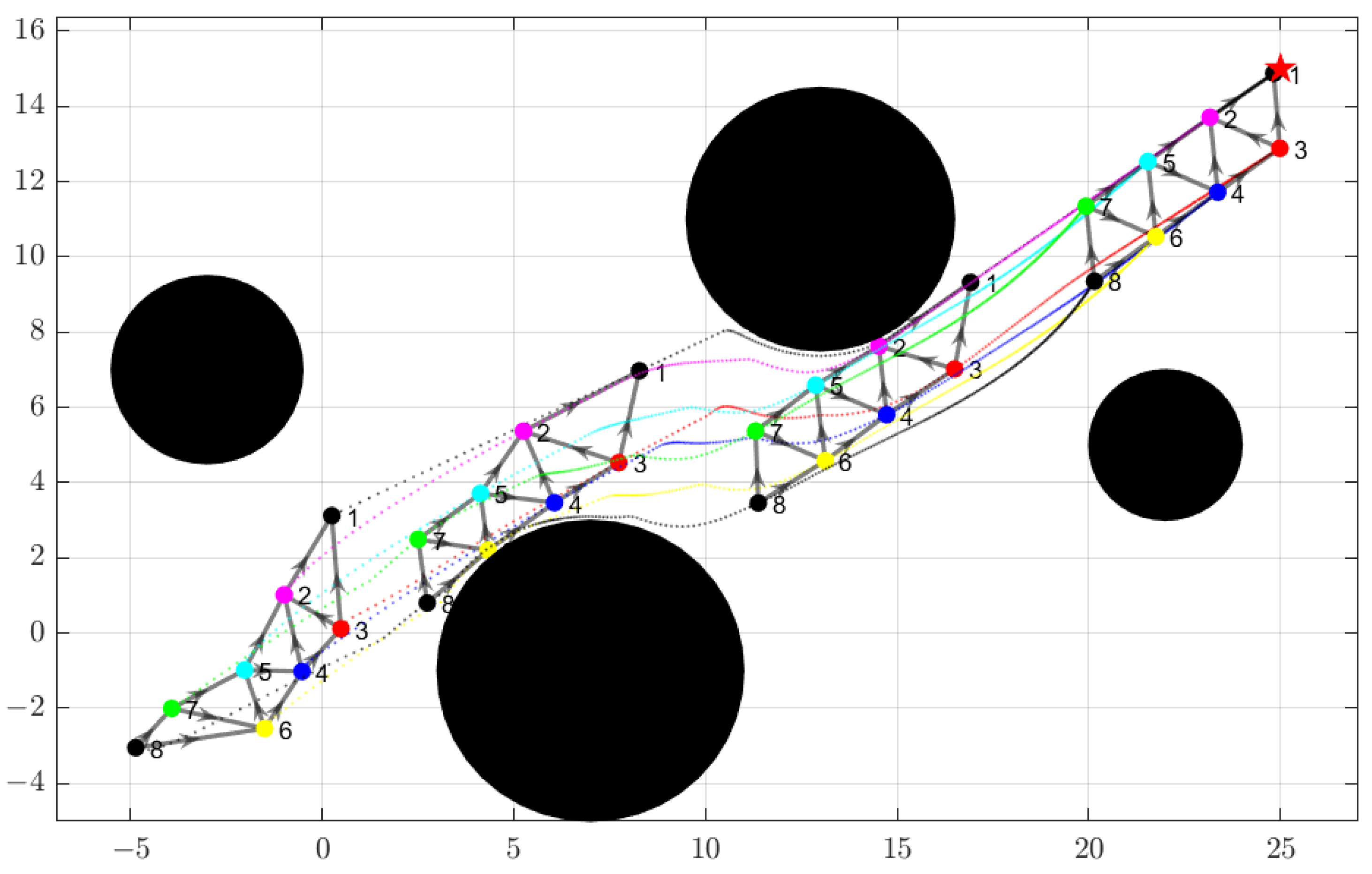
4.1.1. Minimally FOV Persistent Graph

Consider a group of 5 {resp., $30,50$, and $100\}$ robots randomly distributed in a square area with $-10$ and 10 as its bounds in both x- and y-directions. Let the sensing range $R=10$ and the FOV $\alpha =\pi$. The generated minimally persistent graphs are shown in Figure 4. It can be checked that the resultant sparse graphs are all minimally FOV persistent.

When a new robot is added to $G_{FOV}$, there are increases at most $n^{\prime }-1$ candidate edges. For each candidate edge, the complexity of determining whether it can be added to $G_{FOV}$ (via running $Edge\_independence\_test(i,j)$) is $O\left(n^{\prime }\right)$. Therefore, the computational complexity of the proposed FOV pebble game is $O\left(n^2\right)$.

The relationship between the runtime of the algorithm and the number of robots is shown in Figure 5. As the number of robots increases, the time to generate graphs increases accordingly. Note that when the FOV is larger than $\pi$, the FOV constraints is naturally satisfied during pebble searching because the largest angle formulated by a robot and its outward and inward neighbors is $\pi$. In this situation, only the sensing range needs to be considered, so the proposed DFS-based algorithm degenerates to that in [23]. From this point of view, the modified pebble game can be regarded as a special case of our proposed FOV pebble game.

4.1.2. Formation Control

We demonstrate the effectiveness of the formation control scheme in four different cases. The first simulation is conducted in the obstacle free environment. Formation generation and control in sparse and dense obstacle environments are considered in the second and third cases, respectively. The above three simulations are carried out in MATLAB. In order to compensate for the gap between numerical simulations and physical experiments, the fourth case is conducted in the Gazebo simulator in which both vision-based relative position estimation and real dynamics of quadrotors are considered.

Case a: Given a team of 9 robots with randomly initialized positions in the obstacle free environment, the minimally FOV persistent graph is generated shown in Figure 6. The resultant graph presents the LFF structure, where robots 8 and 7 are the global leader and first follower, respectively, and others are ordinary followers. The desired distance between each connected pair robots is set as 3 m. The sensing range and the FOV are set as 5 m and $\frac{\pi }{2}$, respectively. $k_u$ is chosen to be $0.5$. To clearly show the formation evolution using the controller (12), we assign an extra velocity $[-1,0.3$sin${\left(0.8t\right)]}^{\mathrm{T}}$ to each robot. As shown in Figure 6, the desired formation is realized. Figure 7 shows the sum of distance errors ${\sum }_{i=1}^9{\sum }_{j=1}^{n_i}|\parallel {\gamma }_{ij}\parallel -d_{ij}|$, where $n_i$ denotes the number of robot i’s neighbors. It can be seen that the total distance errors gradually converges to 0 as the formation is formed.

Case b: In this case, a known environment with sparse obstacles is considered. Assume that a team of eight robots enters this environment and navigates to the target position in the desired formation. There are four obstacles of different sizes in this environment. In the real environment, obstacles of other shapes can also be surrounded by circles. Therefore, here we assume that the obstacles are all circular. We set the desired distance $d_{ij}=2$ m, sensing range $R=6$ m, $\alpha =\frac{\pi }{2}$, safe distance $r=0.1$ m, $k_u=5$, and $\delta =1.2$. First of all, the minimally persistent graph is generated as shown in the lower left of Figure 8. Robot 1, marked by a black dot, is the leader whose target position is $(25,15)$ marked by a red star. Four solid black circles denote obstacles whose radius are $2.5$, 4, $3.5$, and 2 m, respectively. ${\Delta }_{ob}$ is chosen to be 0.3. As shown in Figure 8, obstacles can be avoided by the QP-based controller (12) as the formation moves towards the desired position. The black arrows in Figure 9 represent the sensing topology which do not changed, namely, the visual constraints can always be satisfied. Finally, the formation converges to the desired formation after traversing the obstacle area. Figure 9 shows the sum of distance errors ${\sum }_{i=1}^8{\sum }_{j=1}^{n_i}|\parallel {\gamma }_{ij}\parallel -d_{ij}|$. It can be seen that as the formation approaches the obstacle, the error increases because the robot takes collision avoidance actions. When passing the obstacle, the robots control themselves to form the desired distance from their neighbors, and eventually the formation error converges to 0 representing the realization of the desired formation.

Case c: In this case, we aim to show that the introduction of obstacles may cause the proposed controller invalid. Consider a scenario that four robots are randomly distributed in an area with dense obstacles. First, the minimally FOV persistent graph is generated by Algorithm 1 with robot 1 being the leader as shown in Figure 10a. In our settings, robot 1 is separately navigated by appropriate control algorithms to the target position denoted by a red star. When obstacles become denser, the robots may fail to satisfy the visual constraints and collision avoidance at the same time. This is because the dense obstacle environment restricts the area where the formation can safely pass, reducing the area in which each robot can move. In this case, the motion of the robot’s neighbors may cause its own safe set to approach the empty set, which may lead to an infeasible QP. It can be seen that at about $t=0.7$ s, no solution exists for robot 3, namely, the safe set is empty. In this situation, the sensing topology must be accordingly changed to continue the prescribed mission. Here we let the robot follow the nearest neighbor, so robot 3 follows robot 2. The altered topology is illustrated in Figure 10b. Similarly, robot 4 chooses to continue tracking robot 3 at $t=0.76$ s as shown in Figure 10c. Figure 10d illustrates the sensing topology at the end. It can be seen that the mission can be accomplished via altering the sensing topology.

Case d: In this case, a robotic simulation is conducted in Gazebo on ROS. Gazebo can be used with PixHawk’s firmware to simulate the real dynamics of quadrotors. Figure 11 shows the simulation environment with four quadrotors, where each quadrotor is identified by the colored ball on its head. They are also used to estimate the relative position with respective to the neighbors by using ellipse fitting in OpenCV. Without loss of generality, the estimated position and the ground truth of quadrotor 2 are illustrated in Figure 12. The blue and red lines denote the true and estimated $x,y$-coordinates, respectively. Note that at about $t=8$ s, the minimally persistent graph is generated and the neighbor can be sensed by quadrotor 2. In this case, we set the desired distance $d_{ij}=2.5$ m, sensing range $R=5$ m, $\alpha =\frac{\pi }{2}$, safe distance $r=0.2$ m, $k_u=0.5$, and $\delta =0.5$. The evolution of formation is illustrated in Figure 13. Figure 14 shows the trajectories of four quadrotors and the internal angle formed by their neighbors. It is shown that the angle of each quadrotor does not exceed the FOV. Despite the noise in the sensing information, the proposed algorithm is able to achieve safe formation control without communication by carefully setting the parameters.

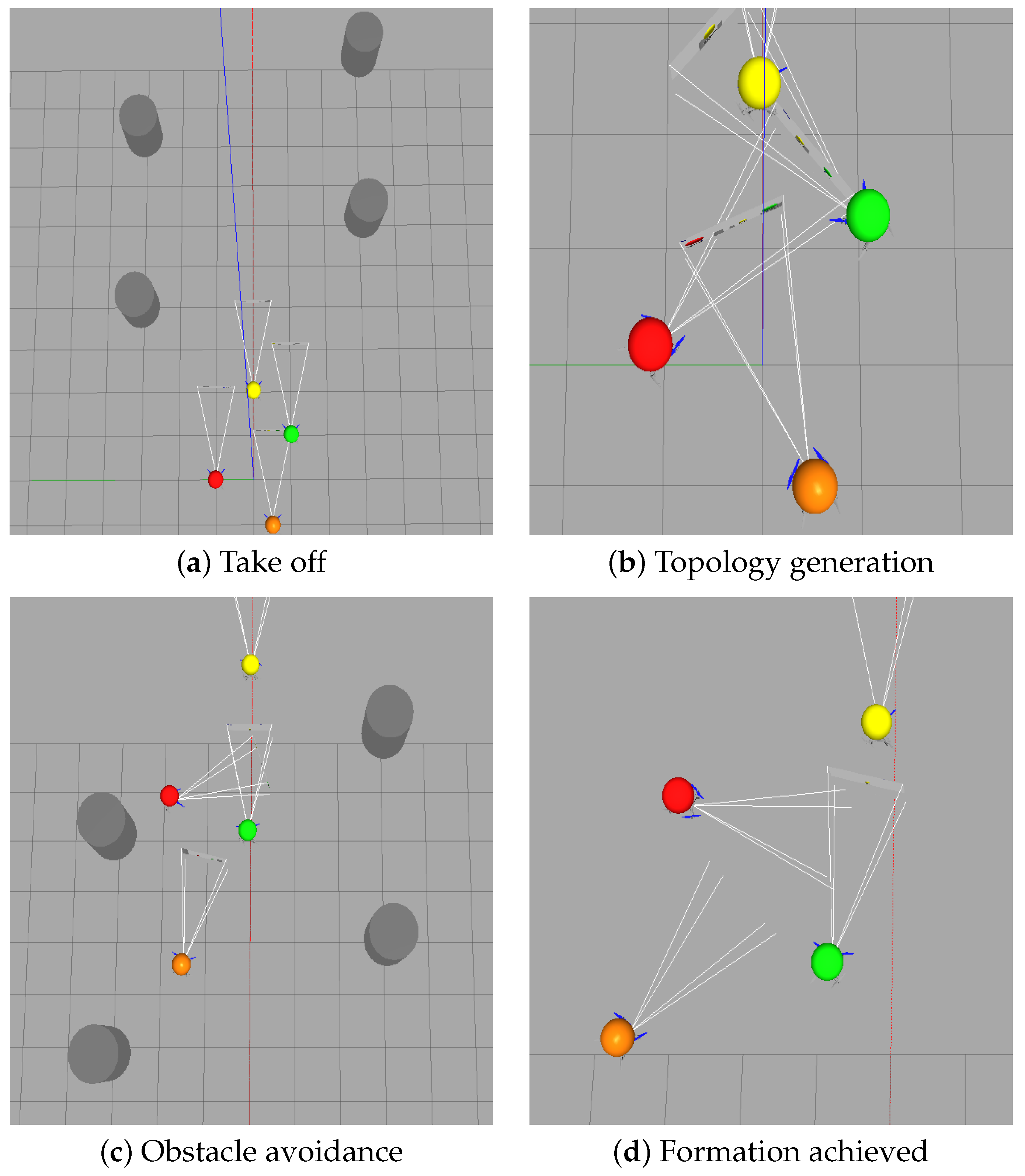
4.2. Experimental Results

The experiment consists of three quadrotors with flight controller Pixhawk 4. Each quadrotor is equipped with an onboard computer NVIDIA Jetson Xavier NX for online processing and an Intel T265 for self-localization. In addition, an Aruco marker [38] and a web camera with an ${85}^{\circ }$ FOV horizontally are mounted at the top of each quadrotor for estimating the relative position. The software implementation is in Prometheus (an open source software for autonomous drones [39]) under Ubuntu 18.04, melodic release. The ground truth positions of quadrotors are recorded by NOKOV Motion Capture System. A ground station is used to send the state transition commands to each quadrotor. The experiment setup is shown in Figure 15. Moreover, an open-source QP solver qpOASES [40] based on online active set strategy is used for solving controller (12).

In the experiment, the frequency of the relative position estimation algorithm and the control algorithm is 17 and 20Hz, respectively. At the beginning, three quadrotors are randomly distributed as shown in Figure 16a. Yellow arrows in Figure 16b show the generated minimally persistent graph. Finally, Figure 16c shows the formed formation. Figure 17 illustrates the trajectories of three quadrotors and the formation errors between each pair of quadrotors. To verify that controller (12) can preserve the visual constraints, at about $t=60$ s, quadrotor 2 is controlled a larger distance to quadrotor 1. In order to meet the visual constraints, quadrotor 3 adjusts its distance with quadrotors 1 and 2 accordingly. Then, quadrotor 2 converges to the desired distance to quadrotor 1. It can be observed that the desired formation is reached with small distance errors that are unavoidable in physical experiments due to the potential disturbances and uncertainties. In fact, excessive disturbance and noise can cause the quadrotor to briefly fly out of the visual range of its neighbors, i.e., outside the safety set. However, due to the robustness of the CBF, the quadrotor will converge to the safe set when the observation is stable. In the experiments, it can be ensured that the neighbors are always in the visual range by increasing the quadrotor recognition speed and setting a threshold for target loss. One can also see that there exists a sharp slope at about $t=90$ s, it occurred due to the date loss from NOKOV. This phenomena is also observed in other time instants. The flight modes and first-person view of the quadrotors during formation are monitored by NoMachine as shown in Figure 18. The experimental results confirm the effectiveness of the algorithm.

5. Conclusions

In this paper, a DFS-based algorithm has been proposed to generate a minimally FOV persistent graph for a group of arbitrarily distributed robots in the plane. It is shown that the resultant graph is consistent with robots’ limited sensing constraints, namely the field of view and range. Then, in combination with the gradient descent control technique and CBF, we have designed a distributed control framework, where the control law is derived based on the nominal controller under the sensing connectivity constraints. Finally, we have theoretically shown that for feasible formation shapes that are compatible with robots’ intrinsic sensing constraints; the desired formations can be achieved using the proposed control scheme, which is further verified by simulations and experiment. The convergence of the formation error for different cases proves the effectiveness of the proposed algorithm. In future work, we will consider the three-dimensional formation control problem under sensing noises.

References

1. Wang, J.; Ding, X.; Wang, C.; Liang, L.; Hu, H. Affine formation control for multi-agent systems with prescribed convergence time. J. Frankl. Inst. 2021, 358, 7055–7072. [Google Scholar] [CrossRef]
2. Li, Q.; Hua, Y.; Dong, X.; Yu, J.; Ren, Z. Time-Varying Formation Tracking Control for Unmanned Aerial Vehicles with the Leader’s Unknown Input and Obstacle Avoidance: Theories and Applications. Electronics 2022, 11, 2334. [Google Scholar] [CrossRef]
3. Wen, J.; Yang, J.; Li, Y.; He, J.; Li, Z.; Song, H. Behavior-Based Formation Control Digital Twin for Multi-AUG in Edge Computing. IEEE Trans. Netw. Sci. Eng. 2022. [Google Scholar] [CrossRef]
4. Fu, H.; Wang, S.; Ji, Y.; Wang, Y. Formation Control of Unmanned Vessels with Saturation Constraint and Extended State Observation. J. Mar. Sci. Eng. 2021, 9, 772. [Google Scholar] [CrossRef]
5. Oh, K.K.; Park, M.C.; Ahn, H.S. A survey of multi-agent formation control. Automatica 2015, 53, 424–440. [Google Scholar] [CrossRef]
6. Yan, Z.; Jiang, A.; Lai, C.; Li, H. Velocity-Free Formation Control and Collision Avoidance for UUVs via RBF: A High-Gain Approach. Electronics 2022, 11, 1170. [Google Scholar] [CrossRef]
7. Yang, Q.; Fang, H.; Cao, M.; Chen, J. Planar Affine Formation Stabilization via Parameter Estimations. IEEE Trans. Cybern. 2022, 52, 5322–5332. [Google Scholar] [CrossRef]
8. Xiao, F.; Yang, Q.; Zhao, X.; Fang, H. A Framework for Optimized Topology Design and Leader Selection in Affine Formation Control. IEEE Robot. Autom. Lett. 2022, 7, 8627–8634. [Google Scholar] [CrossRef]
9. Zhang, P.; Chen, G.; Li, Y.; Dong, W. Agile Formation Control of Drone Flocking Enhanced With Active Vision-Based Relative Localization. IEEE Robot. Autom. Lett. 2022, 7, 6359–6366. [Google Scholar] [CrossRef]
10. Kabore, K.M.; Güler, S. Distributed Formation Control of Drones With Onboard Perception. IEEE/ASME Trans. Mechatron. 2022, 27, 3121–3131. [Google Scholar] [CrossRef]
11. Wang, Y.; Shan, M.; Yue, Y.; Wang, D. Vision-Based Flexible Leader–Follower Formation Tracking of Multiple Nonholonomic Mobile Robots in Unknown Obstacle Environments. IEEE Trans. Control Syst. Technol. 2020, 28, 1025–1033. [Google Scholar] [CrossRef]
12. Li, X.; Tan, Y.; Mareels, I.; Chen, X. Compatible Formation Set for UAVs with Visual Sensing Constraint. In Proceedings of the 2018 Annual American Control Conference (ACC), Milwaukee, WI, USA, 27–29 June 2018; pp. 2497–2502. [Google Scholar] [CrossRef]
13. Liu, X.; Ge, S.S.; Goh, C.H. Vision-Based Leader–Follower Formation Control of Multiagents With Visibility Constraints. IEEE Trans. Control Syst. Technol. 2019, 27, 1326–1333. [Google Scholar] [CrossRef]
14. Miao, Z.; Zhong, H.; Lin, J.; Wang, Y.; Chen, Y.; Fierro, R. Vision-Based Formation Control of Mobile Robots With FOV Constraints and Unknown Feature Depth. IEEE Trans. Control Syst. Technol. 2021, 29, 2231–2238. [Google Scholar] [CrossRef]
15. Mukherjee, P.; Santilli, M.; Gasparri, A.; Williams, R.K. Distributed Adaptive and Resilient Control of Multi-Robot Systems With Limited Field of View Interactions. IEEE Robot. Autom. Lett. 2022, 7, 5318–5325. [Google Scholar] [CrossRef]
16. Dai, S.L.; Lu, K.; Jin, X. Fixed-Time Formation Control of Unicycle-Type Mobile Robots with Visibility and Performance Constraints. IEEE Trans. Ind. Electron. 2021, 68, 12615–12625. [Google Scholar] [CrossRef]
17. Yang, Q.; Cao, M.; Fang, H.; Chen, J. Constructing Universally Rigid Tensegrity Frameworks With Application in Multiagent Formation Control. IEEE Trans. Autom. Control 2019, 64, 381–388. [Google Scholar] [CrossRef] [Green Version]
18. Jacobs, D.J.; Hendrickson, B. An Algorithm for Two-Dimensional Rigidity Percolation: The Pebble Game. J. Comput. Phys. 1997, 137, 346–365. [Google Scholar] [CrossRef]
19. Hendrickx, J.M.; Anderson, B.D.O.; Delvenne, J.C.; Blondel, V.D. Directed graphs for the analysis of rigidity and persistence in autonomous agent systems. Int. J. Robust Nonlinear Control 2007, 17, 960–981. [Google Scholar] [CrossRef]
20. Hendrickx, J.; Fidan, B.; Yu, C.; Anderson, B.; Blondel, V. Elementary Operations for the Reorganization of Minimally Persistent Formations. In Proceedings of the International Symposium on Mathematical Theory of Networks and Systems (MTNS 2006), Kyoto, Japan, 24–28 July 2006; pp. 859–873. [Google Scholar]
21. Yu, D.; Chen, C.L.P. Automatic Leader–Follower Persistent Formation Generation With Minimum Agent-Movement in Various Switching Topologies. IEEE Trans. Cybern. 2020, 50, 1569–1581. [Google Scholar] [CrossRef]
22. Luo, X.-Y.; Li, S.-B.; Guan, X.-P. Automatic generation of min-weighted persistent formations. Chin. Phys. B 2009, 18, 3104. [Google Scholar] [CrossRef]
23. Smith, B.S.; Egerstedt, M.; Howard, A. Automatic Generation of Persistent Formations for Multi-Agent Networks Under Range Constraints. Mob. Netw. Appl. 2009, 14, 322–335. [Google Scholar] [CrossRef] [Green Version]
24. Luo, X.; Li, S.; Guan, X. Automatic generation of minimally persistent formations using rigidity matrix. In Proceedings of the 2009 IEEE Intelligent Vehicles Symposium, Xi’an, China, 3–5 June 2009; pp. 1198–1203. [Google Scholar] [CrossRef]
25. Wang, H.; Guo, Y. Minimal persistence control on dynamic directed graphs for multi-robot formation. In Proceedings of the 2012 IEEE International Conference on Robotics and Automation, Saint Paul, MN, USA, 14–18 May 2012; pp. 1557–1563. [Google Scholar] [CrossRef] [Green Version]
26. Borrmann, U.; Wang, L.; Ames, A.D.; Egerstedt, M. Control Barrier Certificates for Safe Swarm Behavior. IFAC-PapersOnLine 2015, 48, 68–73, Analysis and Design of Hybrid Systems ADHS. [Google Scholar] [CrossRef]
27. Son, T.D.; Nguyen, Q. Safety-Critical Control for Non-affine Nonlinear Systems with Application on Autonomous Vehicle. In Proceedings of the 2019 IEEE 58th Conference on Decision and Control (CDC), Nice, France, 11–13 December 2019; pp. 7623–7628. [Google Scholar] [CrossRef]
28. Zheng, D.; Wang, H.; Wang, J.; Zhang, X.; Chen, W. Toward Visibility Guaranteed Visual Servoing Control of Quadrotor UAVs. IEEE/ASME Trans. Mechatron. 2019, 24, 1087–1095. [Google Scholar] [CrossRef]
29. Laman, G. On graphs and rigidity of plane skeletal structures. J. Eng. Math. 1970, 4, 331–340. [Google Scholar] [CrossRef]
30. Hendrickx, J.M.; Fidan, B.; Yu, C.; Anderson, B.D.O.; Blondel, V.D. Primitive operations for the construction and reorganization of minimally persistent formations. arXiv 2006, arXiv:cs/0609041. [Google Scholar]
31. Wieland, P.; Allgöwer, F. Constructive safety using control barrier functions. IFAC Proc. Vol. 2007, 40, 462–467. [Google Scholar] [CrossRef]
32. Ames, A.D.; Grizzle, J.W.; Tabuada, P. Control barrier function based quadratic programs with application to adaptive cruise control. In Proceedings of the 53rd IEEE Conference on Decision and Control, Los Angeles, CA, USA, 15–17 December 2014; pp. 6271–6278. [Google Scholar] [CrossRef]
33. Ames, A.D.; Xu, X.; Grizzle, J.W.; Tabuada, P. Control Barrier Function Based Quadratic Programs for Safety Critical Systems. IEEE Trans. Autom. Control 2017, 62, 3861–3876. [Google Scholar] [CrossRef]
34. Ames, A.D.; Coogan, S.; Egerstedt, M.; Notomista, G.; Sreenath, K.; Tabuada, P. Control Barrier Functions: Theory and Applications. In Proceedings of the 2019 18th European Control Conference (ECC), Naples, Italy, 25–28 June 2019; pp. 3420–3431. [Google Scholar] [CrossRef] [Green Version]
35. Summers, T.H.; Yu, C.; Dasgupta, S.; Anderson, B.D.O. Control of Minimally Persistent Leader-Remote-Follower and Coleader Formations in the Plane. IEEE Trans. Autom. Control 2011, 56, 2778–2792. [Google Scholar] [CrossRef]
36. Wang, L.; Ames, A.; Egerstedt, M. Safety barrier certificates for heterogeneous multi-robot systems. In Proceedings of the 2016 American Control Conference (ACC), Boston, MA, USA, 6–8 July 2016; pp. 5213–5218. [Google Scholar] [CrossRef] [Green Version]
37. Fu, J.; Lv, Y.; Wen, G.; Yu, X. Local Measurement Based Formation Navigation of Nonholonomic Robots With Globally Bounded Inputs and Collision Avoidance. IEEE Trans. Netw. Sci. Eng. 2021, 8, 2342–2354. [Google Scholar] [CrossRef]
38. Garrido-Jurado, S.; Muñoz-Salinas, R.; Madrid-Cuevas, F.; Marín-Jiménez, M. Automatic generation and detection of highly reliable fiducial markers under occlusion. Pattern Recognit. 2014, 47, 2280–2292. [Google Scholar] [CrossRef]
39. Amovlab. Prometheus Autonomous UAV Opensource Project. Available online: https://github.com/amov-lab/Prometheus (accessed on 1 October 2021).
40. Ferreau, J.; Kirches, C.; Potschka, A.; Bock, H.; Diehl, M. qpOASES: A parametric active-set algorithm for quadratic programming. Math. Programm. Comput. 2014, 6, 327–363. [Google Scholar] [CrossRef]
Figure 1. Two minimally persistent graphs. (a) A general minimally persistent graph that may not satisfy FOV constraints. For instance, assume that α is π 2 and the sensing range R is large enough, the internal angle marked by red dotted line is greater than π 2 . (b) A minimally FOV persistent graph, each internal angle formed by two outward edges is no more than π 2 .
Electronics 12 00317 g001
Figure 2. A scenario of the existence of the fixed pebble. (a) Existing directed graph before pebble searching operation. (b) A fixed pebble is recorded after searching operation.
Electronics 12 00317 g002
Figure 3. Example of sensing constraints with the FOV α < π and the sensing range R. When robot i lies in the green shaded area, its two neighbors can always be observed.
Electronics 12 00317 g003
Figure 4. Generated minimally FOV persistent graphs using 5 {resp., 30 , 50 , and 100 } robots when the sensing range R = 10 and the FOV α = π . (a) 5 robots, (b) 30 robots, (c) 50 robots, and (d) 100 robots.
Electronics 12 00317 g004
Figure 5. Relationship between the runtime of algorithm and the number of robots.
Electronics 12 00317 g005
Figure 6. Formation evolution of 9 robots. Blue graph on the right side shows the initial state of the robot team. On the left side, the robot team is stabilized to the desired formation colored in orange. The intermediate lines represent robot’s trajectories.
Electronics 12 00317 g006
Figure 7. The sum of distance errors of 9 robots.
Electronics 12 00317 g007
Figure 8. Eight robots navigate in a known environment with sparse obstacles. The red star stands for the target position of leader. Solid black circles denote obstacles of different sizes. Eight small colored circles represent robots. The sensing topologies at t = 0 , 0.8 , 2.4 , and 10 s are plotted from left lower to right upper and the dotted line represents the trajectories of four robots.
Electronics 12 00317 g008
Figure 9. The sum of distance errors of 8 robots.
Electronics 12 00317 g009
Figure 10. Four robots navigate in a known environment with dense obstacles. Solid black circles denote obstacles with radius r = 0.6 m. Four small colored circles represent robots. The sensing topologies at t = 0 , 0.7 , 0.76 , and 6 s are plotted. (a) t = 0 s, (b) t = 0.7 s, (c) t = 0.76 s, and (d) t = 6 s.
Electronics 12 00317 g010
Figure 11. Gazebo simulation environment with four quadrotors.
Electronics 12 00317 g011
Figure 12. Comparison of true and estimated coordinates. (a) True and estimated x-coordinate and (b) y-coordinate of quadrotor 2.
Electronics 12 00317 g012
Figure 13. Four quadrotors navigate in a known environment in Gazebo. (a) Four quadrotors take off from the initial position. (b) A minimally persistent graph is generated and the quadrotors turn to the desired orientation. (c) Formation with obstacle avoidance. (d) The leader quadrotor arrives the target position, and the desired formation is realized.
Electronics 12 00317 g013
Figure 14. Trajectories and internal angle of four quadrotors. (a) Trajectories of four quadrotors. (b) Internal angle of four quadrotors formed by the neighbors with upper bound indicated FOV constraints.
Electronics 12 00317 g014
Figure 15. Experiment setup.
Electronics 12 00317 g015
Figure 16. Experimental results. (a) Initialization of formation configuration. (b) Generation of minimally persistent graph. (c) Realization of the desired formation.
Electronics 12 00317 g016
Figure 17. Formation trajectories and errors. (a) Trajectories of three quadrotors recorded by motion capture system. (b) Formation errors between each pair of quadrotors.
Electronics 12 00317 g017
Figure 18. First-person view of the quadrotors during formation.
Electronics 12 00317 g018
Disclaimer/Publisher’s Note: The statements, opinions and data contained in all publications are solely those of the individual author(s) and contributor(s) and not of MDPI and/or the editor(s). MDPI and/or the editor(s) disclaim responsibility for any injury to people or property resulting from any ideas, methods, instructions or products referred to in the content.