Article

Fault Diagnosis of Diesel Engine Valve Clearance Based on Wavelet Packet Decomposition and Neural Networks

1
Faculty of Information Engineering and Automation, Kunming University of Science and Technology, Kunming 650504, China
2
Faculty of Civil Aviation and Aeronautics, Kunming University of Science and Technology, Kunming 650504, China
*
Author to whom correspondence should be addressed.
Electronics 2023, 12(2), 353; https://doi.org/10.3390/electronics12020353
Submission received: 11 November 2022 / Revised: 5 January 2023 / Accepted: 6 January 2023 / Published: 10 January 2023

Abstract

:
In order to improve the accuracy of engine valve clearance fault diagnosis, in this study, a fault identification algorithm based on wavelet packet decomposition and an artificial neural network is proposed. Firstly, the vibration signals of the engine cylinder head were collected, and different levels of noise were superimposed on the extended data sets. Then, the test data were decomposed into wavelet packets, and the power spectrum of the sub-band signal was analyzed using the autoregressive power spectrum density estimation method. A group of values were obtained from the power spectrum integration to form the fault eigenvalue. Finally, a neural network model was designed to classify the fault eigenvalues. In the training process, the test data set was divided into three parts, the training set, the verification set, and the test set, and the dropout layer was added to avoid the overfitting phenomenon of the neural network. The experimental results show that the wavelet packet neural network model in this paper has a good diagnostic accuracy for data with different levels of noise.

1. Introduction

The function of the diesel engine valve mechanism is to control the intake of combustible gas mixtures and exhaust gas. When valve clearance deviates from its normal state, this leads to air leakage, insufficient combustion, engine power decline, increased fuel consumption and other failures, and even serious accidents. Therefore, it is necessary to carry out state detection and fault diagnosis. A key research method is the detection of vibration signals, which has the advantages of fast aging, early fault detection, and no damage.
The vibration signals of the diesel engine cylinder head contain rich and complex information. If the valve clearance deviates from the normal value, the vibration signal will inevitably change. In the literature, the authors of [1] proposed that the change in valve clearance will lead to an increased valve impact on the time-domain signal. The authors of [2] proposed that an increase in the gap leads to an increase of 6~8 kHz energy moment through wavelet packet decomposition. Therefore, how to extract the time-domain, frequency-domain, and time–frequency eigenvalues of the fault signals is a focus of research in this field. The authors of [3] realized valve fault diagnosis by using local mean decomposition edge spectrum and Markov distance to process the signal; the authors of [4,5] decomposed the diesel engine valve signal by using the VMD algorithm of the variational mode decomposition, and then compared the permutation entropy values of different component signals, selected the fault component, and obtained the fault eigenvalue; the authors of [5,6] proposed the use of support vector machine (SVM) fuzzy C-means to extract the valve clearance fault features of diesel engines. The authors of [7,8] used Hilbert–Huang transform to analyze the engine vibration signals and extract the valve fault features. Considering that diesel engine misfire is difficult to diagnose under strong noise interference, a diesel engine misfire fault diagnosis method based on VMD and cross wavelet transform (XWT) was proposed [9,10]. The authors of [11] proposed linear regression for the diagnosis and prediction of valve clearance faults. However, the experiment showed that these methods can be inaccurate when applied to the process of diesel engine valve clearance faults. One of the reasons for this is that noise has a great impact on the accuracy of diagnosis; that is, when the signal-to-noise ratio is low, the accuracy of the diagnosis will drop sharply, making the methods invalid. For example, when the SNR is −5 dB, the accuracy of VMD is only 53%. The main contributions of this work are as follows:
(1)
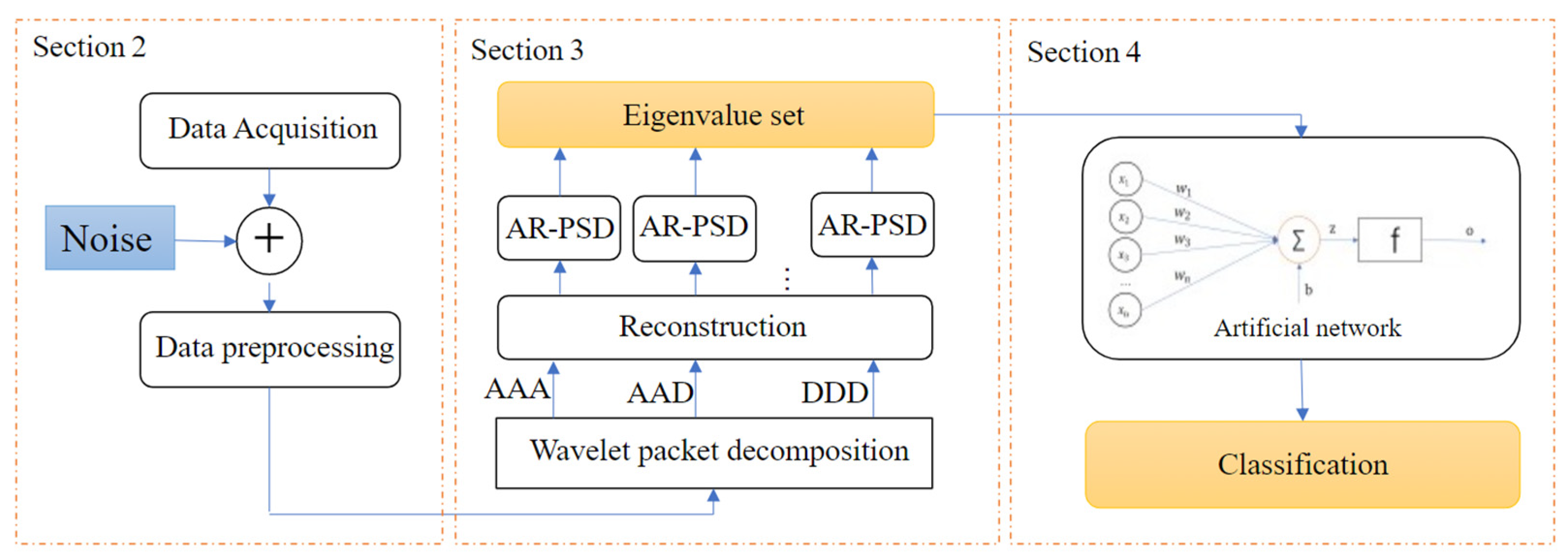
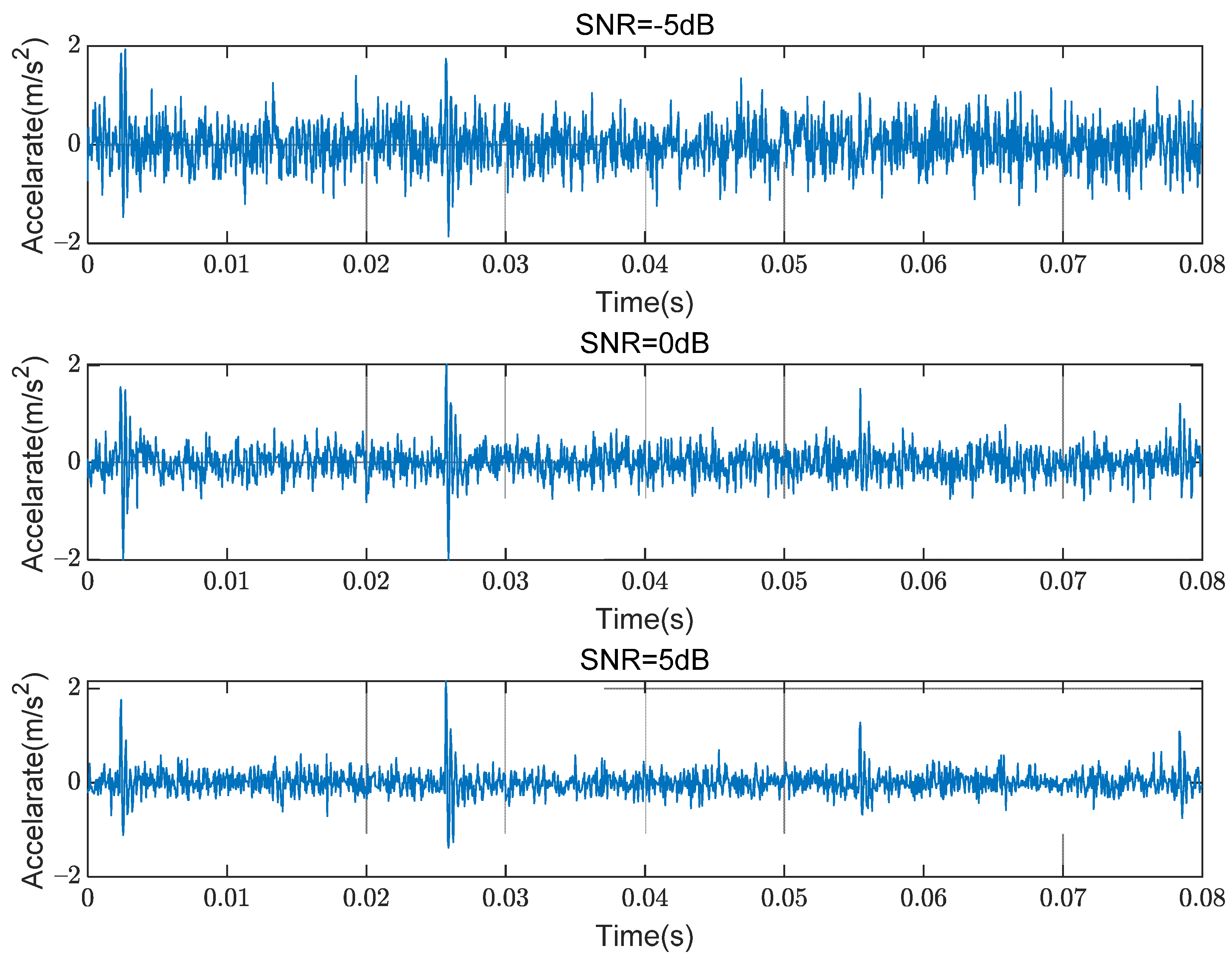
In this paper, a method of mixed training for the model by injecting different levels of noise is proposed, so that the model has a better diagnostic accuracy for fault signals with different levels of noise. In the experiment, nine kinds of valve clearance deviation states were set, and different noises were injected into the collected data to expand the data set. The wavelet packet decomposition algorithm was used to decompose the time-domain signal into three layers of eight frequency sub-band signals. The autoregressive power spectrum density estimation was used to analyze the power spectrum of the sub-band signal, and then the power spectrum integral of each sub-band signal was used to obtain the energy value of the sub-band signal. In this way, eight values could be obtained as the fault eigenvalue of the signal.
(2)
A neural network model was designed using the TensorFlow machine learning platform to classify the fault eigenvalues. During the training process, the test data set was divided into three parts, namely the training set, the verification set, and the test set, and the dropout layer was added to avoid the overfitting phenomenon of the neural network. Finally, the average accuracy of the experimental model reached 82.4%, and achieved good experimental results.
The rest of this paper is organized as the below block diagram in Figure 1. Section 2 introduces the vibration signal acquisition, including the diesel engine, dynamometer, and acceleration signal acquisition equipment. Section 3 describes the wavelet packet decomposition and eigenvalue extraction of the vibration signals. Section 4 introduces the establishment and training of the artificial neural network, and reports the experimental results. Finally, Section 5 summarizes this paper and draws the advantages compared with other methods.
In this paper, an acceleration sensor is used for the signal acquisition, which is a micro electro mechanical system (MEMS), and digital signal processing technology is mainly used, which is also the basic discipline of electronics.

2. Data Acquisition of Valve Clearance Fault

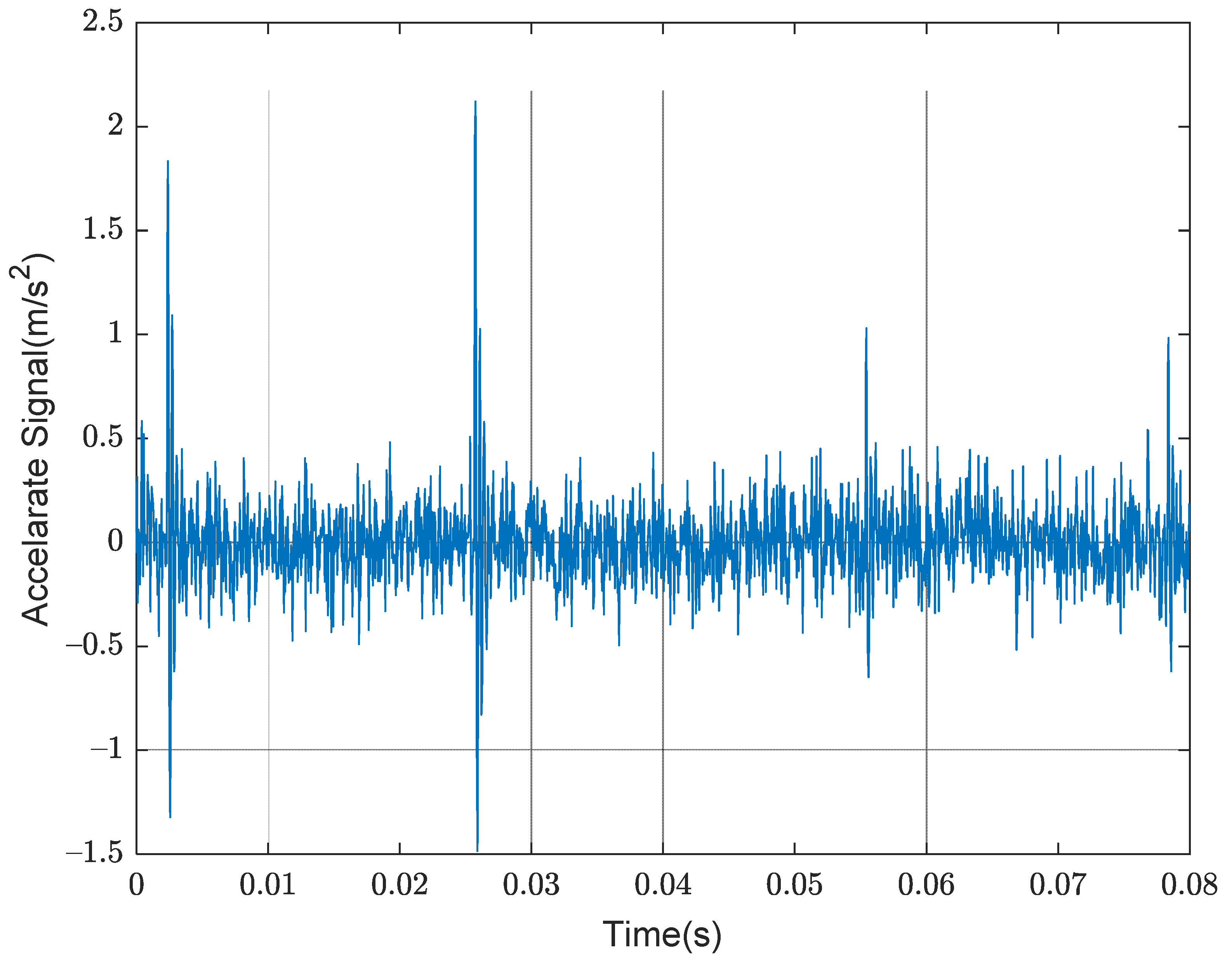
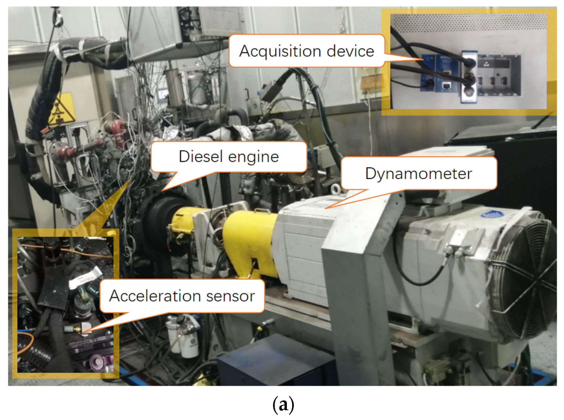
2.1. Vibration Signal Acquisition

The vibration signal of a diesel engine contains rich and complex information [12]. When the inlet valve or exhaust valve clearance deviates from the normal value, the timing sequence and amplitude of the vibration signal generated by the valve seating impact will change slightly [13,14]. In order to study the valve clearance deviation states, the fault simulation of the diesel engine valve was carried out according to Table 1.
Nine states can be obtained by combining the inlet valve clearance and exhaust valve clearance, of which only one is normal, marked as H, and the other eight are fault states, marked as F1, F2, …, F8, respectively, as shown in Table 2.
Cylinder head vibration signals are also affected by the gas combustion excitation force and gas throttling when the exhaust valve is opened. Because of their different action times and different vibration frequency bands, the vibration signals can be separated into time and frequency domains. In this paper, the vibration signal was acquired using motor dragging [1] while disconnecting the fuel of the diesel engine. When this occurs, the main component of the vibration signal is the vibration excitation response generated by the impact of the valve on the cylinder head.
During the acquisition process, the speed of the diesel engine was 1500 r/min, and one working cycle of the engine was 80 ms. When the analog-to-digital converter (ADC) conversion rate was 20 kSPS, 1600 data were collected in each working cycle, referred to as a group of experimental data. A total of 250 groups of experimental data were collected for nine valve clearance combinations. The experimental data were collected using a JDC265 dynamometer from LIANCE Technology with a maximum allowable power of 265 kW. The acceleration sensor was a PCB356A25 and the acquisition module was an NI9232. The diesel engine was a WD615, the rated speed was 2200 rpm, and the power was 210 kW. Figure 2 shows the experimental signal acquisition equipment.
First, the vibration signal within one second is recorded and saved as a file. Then, according to the speed, the signal of a working cycle is calculated. Finally, if the speed is not equal to 1500 rpm, the data need to be interpolated to make it exactly 1600 data points.
Figure 3 shows the time-domain waveform of the vibration signal under the H state.

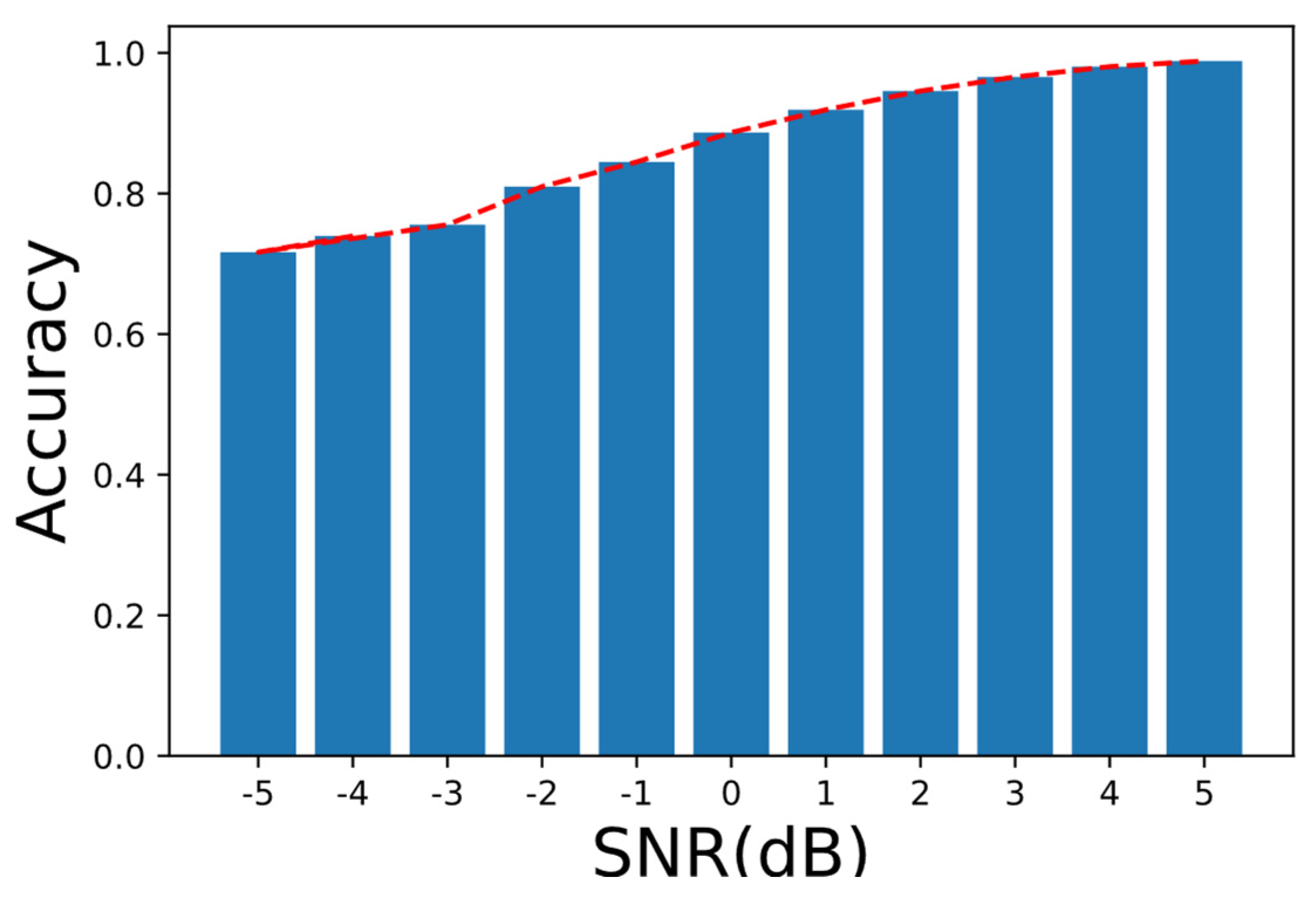
2.2. Noise Injection

To study the adaptability of the neural network model to noisy signals, white gaussian noise must be added to the acquired signals [15].
S = (s1, s2, …, sN) is a group of experimental data, and X~N (0, 1), X = (x1, x2, …, xN) is a group of independent observations of random variable X, SNR = αdB:
P s   = i = 1 N s i 2 N
P x = E ( X 2 ) = D   ( X 2 ) + ( E ( X ) ) 2 =   σ 2
Therefore:
s α dB = s + P s 10 α 10   x
Use Formula (1) to calculate 11 kinds of noisy signals with a signal-to-noise ratio (SNR) ranging from −5 dB to 5 dB, respectively. Each group of noise is generated independently, so each noise superimposed on the signal is different. Figure 4 shows the time-domain waveform of the signal with SNR equal to −5 dB, 0 dB, and 5 dB, respectively, of the H state.

3. Wavelet Packet Decomposition of Vibration Signals

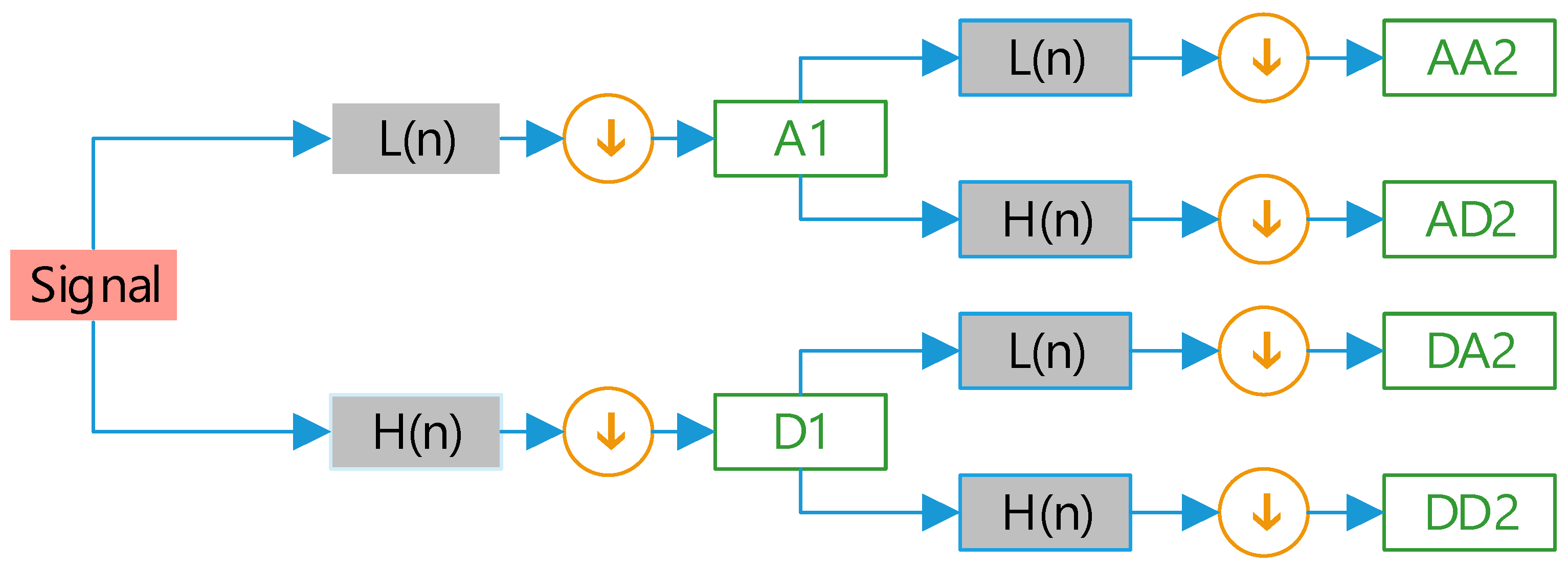
3.1. Wavelet Packet Decomposition

For the wavelet generating formula ψ(t), if function x(t) satisfies square integrability, then the continuous wavelet transform (WT) of x(t) is defined [16,17] as:
C ψ ( f s , f t ) = x ( t ) ψ ( t | f s , f t ) d t
where:
ψ ( t | f s , f t ) = 1 f s ψ ( t f s f t )
where ψ ( t | f s , f t ) is the wavelet function, and   f s , f t are the zoom coefficient and the translation coefficient, respectively.
x(n) is the input signal sequence with length N, and Formula (2) is discretized to obtain the discrete wavelet transform (DWT) [18]:
  A ( n | j , k ) = D S [ n x ( n ) l j * ( n 2 j k ) ]
D ( n | j , k ) = D S [ n x ( n ) h j * ( n 2 j k ) ]
where A represents the low-frequency coefficient; D represents the high-frequency coefficient; l (n) and h (n) represent the low-pass filter and high-pass filter, respectively; l * (n) and h * (n) are conjugate functions of l (n) and h (n), respectively; j and k represent the zoom coefficient and translation coefficient, respectively; and DS represents down-sampling.
Once the input signal is decomposed into the high-frequency sub-band and low-frequency sub-band, respectively, through the above process, then the obtained low frequency sub-band can be employed as the input signal, and wavelet decomposition is then carried out to obtain the next level of high-frequency and low-frequency sub-bands, and so on. With the increase in the progression of wavelet decomposition, the resolution in the frequency domain is also enhanced.
In [16,17], the definition of discrete wavelet packet transform (DWPT) is introduced. DWPT is an expansion and optimization of discrete wavelet transform (DWT). Unlike DWT, at each level of the decomposition process of signals, not only is the low-frequency sub-band further decomposed, but the high-frequency sub-band is further decomposed as well. DWPT calculates the optimal signal decomposition path via minimizing a cost function, which decomposes the signal transmitted in the input channel. Figure 5 shows two-layer wavelet packet decomposition.

3.2. Decomposition of Vibration Signal

The Daubechies wavelet [19] is an orthogonal wavelet referred to as dbN. N is the order of the wavelet. When N increases, the localization of the frequency domain and the division effect of the frequency band are enhanced, but the compact support of the time domain is undermined, the amount of calculation is strengthened, and the real-time performance is impoverished.
Via employing db3 as the wavelet basis function and Shannon entropy as the cost function, the three-layer discrete wavelet packet decomposition was carried out on experimental data with 1600 points in each group, and eight groups of wavelet packet coefficients were obtained. Signal reconstruction was carried out on each group of coefficients to obtain the time-domain signals of eight frequency sub-bands, as shown in Figure 6.

3.3. Power Spectral Density Estimation

The autoregressive model (AR) [20,21] was exploited to estimate the power spectrum of the frequency sub-band of the wavelet packet decomposition. The AR model is an all-pole model, and its signal samples can be expressed as the sum of the weighted combination of several previous samples, the constant, and the error terms. When the sequence is set as x(1), x(2), …, x(N) (n <= N), then x(n) can be obtained by linear weighted prediction of the nearest m samples x(n − 1), x(n − 2), …, x(nm), expressed by the following formula:
x ( n ) = i = 1 m w m ( i ) x ( n i ) + ε ( n )
where m is the order of the model, w m ( i ) is the i-th parameter of the model, and ε ( n ) is the white noise with a mean value of 0 and variance of σ 2 .
The transfer function of the AR model is as follows:
H ( z ) = 1 1 + i = 1 m w m ( i ) z i
The Burg algorithm [20] ensures the stability and reliability of the AR model. This method has a high computational efficiency, high frequency resolution, and is suitable for applications where a high model accuracy is required. The Burg algorithm minimizes the sum of forward and backward errors by calculating the reflection coefficient k m . The coefficient of the m-order AR model is derived recursively from the Levison relational formula:
w m ( i ) = w m 1 ( i 1 ) + k m w m 1 ( i )
According to the obtained parameters, the calculation formula of the power spectral density (PSD) estimation is as follows:
P S D ( k ) = σ 2 | 1 + i = 1 m w m ( i ) W N k i |
where N is the length of the PSD sequence:
W N = e j 2 π N

3.4. Eigenvalue Extraction

AR power spectrum estimation [22] was performed on the time-domain signals of each frequency band, as shown in Figure 7.
The power spectral density function was accumulated to obtain the energy value of the frequency band:
E = k = 1 N P S D ( k )
The authors of [2] proposed that an increase in the gap leads to an increase of 6~8 kHz energy moment through wavelet packet decomposition, so taking this energy value as the eigenvalue of the band signal is reasonable. Eight eigenvalues can be extracted from a group of experimental data to characterize the experiment.
Table 3 shows the eigenvalues of a group of experimental data for each of the nine valve clearance states. The eigenvalues of all 9 × 50 groups of experimental data were analyzed, and Figure 8 shows the correlation (off-diagonal) and distribution (diagonal) of the eigenvalues [23].

4. Establishment of Neural Network

4.1. Establishment of Artificial Neural Network (ANN)

An artificial neural network is a non-linear statistical data operating model that is computed by a large number of nodes (artificial neurons), has a learning function, and is adaptive to external information [24,25,26]. Neural networks have been utilized to resolve problems that are difficult to solve with programming based on traditional rules, such as machine vision and artificial recognition, and have also been used for mechanical fault diagnosis [27,28].
In the neuron model in Figure 9, set X = [x1, x2, …, xn], W = [w1, w2, …, wn], where f is the activation function, then:
o = f ( z ) = f ( w T   x + b )
Commonly used activation functions [17] include Sigmoid, ReLu, LeakyReLu, Tanh, etc. Because the calculation of the function value and derivative value of ReLU is very simple, this can avoid the phenomenon of gradient dispersion and gradient disappearance, so it is an effective activation function.
ReLU ( x ) = max ( 0 , x )
d d x [ ReLU ( x ) ] = { 1 , x 0 0 , x 0
The features of a single neuron are few, but it can be enhanced by stacking multiple neurons in parallel to realize a multi-input and multi-output (MIMO) network layer. A three-layer neural network was created to classify the eigenvalues of the vibration signals extracted in the previous section. As there were eight kinds of input eigenvalues, the number of nodes in the network input layer was eight. Layer one and layer two were hidden layers, with 64 nodes each. The output layer corresponds to nine fault states, which are discrete eigenvalues and adopt one-hot coding, so there were nine nodes. Figure 10 shows the network structure, with 5321 parameters to be trained.
For multi-class classification problems, the output value of each node of the output layer o i represents the conditional probability P ( O i | x ) that the present specimen belongs to O i , so the following constraint conditions need to be met:
o i 1   and   i o i = 1
This can be implemented by adding softmax functions in the output layer. In a TensorFlow [29] machine learning framework, softmax and cross-entropy functions can be realized simultaneously, which avoids exponential operation overflow when the value is large and improves the stability of the numerical calculation.

4.2. Training and Testing

The most common training algorithm of an artificial neural network is the back propagation algorithm (BP algorithm) [24]. The steps of the algorithm are listed as follows:
(1)
Enter the training data x into the network to obtain the excitation output o = f θ ( x ) , f θ ( x )   means a θ parameterized network model.
(2)
Calculate the error between the excitation output and the target output, L = g ( o , y ) , g represents the error function.
(3)
Using TensorFlow automatic derivative technology to obtain the gradient of the θ, θ L = L θ 1 , L θ 2 , , L θ n .
(4)
Update the parameters according to gradient descent algorithm, θ ¯ = θ η * θ L , where η is the learning rate.
Iterate the above steps repeatedly until the error reaches the intended target.
The data set of the experiments was split into three sets: the training set (1350 groups, 60%), the validation set (450 groups, 20%), and the test set (450 groups, 20%). The training set was only employed for the training model parameters; the validation set was not involved in training, and was used to determine network hyperparameters, such as adjusting the topology of the network, adjusting the learning rate, number of training sessions, and judging whether or not it has been over-fitted. The test set was not involved in training, but only utilized to test the generalization of the target model.
Traversing all the samples in the training set at one time is called an epoch. Observing the accuracy indicator of the validation set, if the change value in several consecutive epochs was less than the specified threshold value, it was considered that the training was completed and early stopping could be achieved.
Figure 11 shows the change curve of the loss function (cross entropy) of the training set, validation set, and test set to the epoch, when the input was a data set with SNR = 0 dB. Figure 12 shows the change curve of mean squared error (MSE). Figure 13 shows the change curve of the classification accuracy to the epoch. When the training was completed, the accuracy of the test set was 91.8%.
Eleven types of experimental data sets were trained with SNRs = −5 dB, −4 dB, …, 5 dB, respectively, and the test accuracy at the end of the training was recorded as being 0.769, 0.807, 0.829, 0.873, 0.893, 0.918, 0.951, 0.973, 0.978, 0.980, and 0.982, respectively. The formula for the accuracy was as follows:
A c c u r a c y = N u m b e r   o f   s a m p l e s   i d e n t i f i e d N u m b e r   o f   e x p e r i m e n t a l   s a m p l e s
It can be seen that noise had a significant impact on the accuracy.
To let the artificial neural network classify the experimental data of various SNRs, it was necessary to carry out mixed training on the experimental data of all SNRs. The scale of the mixed data set was 11 times that of the independent training, and the distribution became complex. In this scenario, the training algorithm will obtain unnecessary information from the noise and express it in the model parameters, resulting in the overfitting phenomenon. As shown in Figure 14, the accuracy of the training set in the figure also increased with the magnification of the training epoch, while the accuracy of the verification set and the test set hardly increased, which indicates an overfitting phenomenon.
Adding a dropout layer can effectively avoid overfitting [30]. Dropout is a regularization technique that randomly discards some neurons and updates only some network parameters at a certain probability in the network during each instance of training [31,32]. This makes the network structure different during each instance of training. The updating of weights does not depend on the joint action of hidden nodes with fixed relationships. The whole training process is equivalent to averaging different networks.
A dropout layer with a dropout probability of 0.5 was inserted in front of the second hidden layer, the mixed data set was trained, and an accuracy curve was obtained as shown in Figure 15. When the training was completed, an accuracy of 82.4% was achieved for the test set.
The trained model was used to test the data sets of each SNR, and the accuracy results were 63.9%, 70.1%, 74.7%, 76.1%, 82.0%, 86.0%, 90.2%, 93.4%, 95.7%, 97.1%, and 98.3%, respectively, as shown in Figure 16. The data show that when the SNR value was large (low noise), the classification accuracy of the model was also high.

5. Conclusions

To improve the accuracy of the engine valve clearance fault diagnosis, this paper proposes a fault identification algorithm based on wavelet packet decomposition and an artificial neural network. Compared with Fourier transform, wavelet packet decomposition is a local analysis method of time and frequency. It gradually refines the signal at multiple scales through scaling and translation operations. The time resolution of the high-frequency signal is improved, and when the signal frequency is low, the frequency resolution is high. It can automatically adapt to the requirements of the time–frequency signal analysis, so as to focus on any details of the signal. The vibration signal of the diesel engine cylinder head is decomposed into a multi-level high-frequency sub-band and low-frequency sub-band by a wavelet packet, and then the eigenvalues of the diesel engine valve clearance fault are extracted by the AR power spectral density estimation. The AR-PSD estimation algorithm using the Burg method has a very high-resolution estimation for short data records. Then, a neural network model is used to classify the fault eigenvalues, and the dropout layer is inserted to improve the generalization ability of the model. The algorithm is sensitive, stable, fast and easy to implement. When training the neural network model, the dropout can greatly simplify the neural network structure to prevent over fitting and reduce the time spent in training the neural network model. The neural network expands the data set by injecting noise, and has a good classification accuracy for various SNR fault data. The accuracy of the low noise data set is 98.3% and the average accuracy is 82.4%. Compared with the training model without noise injection, the average accuracy is only 71.1%—an increase of 11.3%. Compared with the VMD method, when SNR is small (−5 dB), the accuracy is improved.
The use of vibration analysis technology for fault diagnosis belongs to non-destructive testing technology, which has the advantages of a low cost and easy realization. It can be used for fault prediction and can prevent major accidents.
The diesel engine in Figure 17a is undergoing reliability tests. We installed an acceleration sensor on the cylinder head to monitor the valve clearance failure. Figure 17b shows the experimental equipment and software.
The research method in this paper can be extended to motor fault diagnosis, bearing defect early warning and coupling misalignment fault detection.
In the future, we will focus on online real-time diagnosis methods and early fault warning of diesel engine valve clearance faults, reducing the complexity and randomness of diagnosis, improving the intelligence of fault diagnosis, and ensuring the detection accuracy.

Author Contributions

Conceptualization, Z.K.; methodology, Z.K. and G.H.; writing—original draft preparation, Z.K.; writing—review and editing, Z.K. and G.H.; resources, Z.K.; software, Z.K. and G.H.; validation, Z.K. and G.H. All authors have read and agreed to the published version of the manuscript.

Funding

This research received no external funding.

Data Availability Statement

All data, models, and code generated or used during the study appear in the submitted article.

Conflicts of Interest

The authors declare no conflict of interest.

References

  1. Fei, H.-Z.; Zhang, S.-J.; Liu, L.; Li, X.-M.; Ma, X.-Z. Study on Feature Extraction for Diesel Engine Valve Faults. Chin. Intern. Combust. Engine Eng. 2016, 37, 145–150. [Google Scholar]
  2. Li, Y.-L.; Wang, L.-Y.; Luan, Z.-G.; Chen, T. Fault Diagnosis of Valve Clearance Based on Time-Domain Characteristics of Vibration. China Pet. Mach. 2014, 42, 48–51. [Google Scholar]
  3. Wang, H.; Wang, L.; Tian, R. Structural damage detection using correlation functions of time domain vibration responses and data fusion. Eng. Mech. 2020, 37, 30. [Google Scholar]
  4. Jiang, Z.; Wei, D.; Zhang, J.; Mao, Z. A study on valve clearance anomaly feature extraction of diesel engines based on VMD and SVD. J. Vib. Shock 2020, 39, 23–30. [Google Scholar]
  5. Bi, F.; Tang, D.; Zhang, L.; Li, X.; Ma, T.; Yang, X. Diesel Engine Fault Diagnosis Method Based on Optimized Variational Mode Decomposition and Kernel Fuzzy C-means Clustering. J. Vib. Meas. Diagn. 2020, 40, 853–858. [Google Scholar]
  6. Sun, T.; Chen, Y.Q.; Zhou, Y. Fault prediction of marine diesel engine based on time series and support vector machine. In Proceedings of the International Conference on Intelligent Design (ICID), Xi’an, China, 11–13 December 2020; pp. 75–81. [Google Scholar] [CrossRef]
  7. Duo, M.; Ji, G. Bearing fault diagnosis based on Hilbert-Huang transform and residual neural network. Manuf. Autom. 2022, 44, 20–23. [Google Scholar]
  8. Liu, Y.L.; Chang, W.B.; Zhang, S.Y.; Zhou, S.H. Fault Diagnosis and Prediction Method for Valve Clearance of Diesel Engine Based on Linear Regression. In Proceedings of the Annual Reliability and Maintainability Symposium (RAMS), Palm Springs, CA, USA, 27–30 January 2020. [Google Scholar]
  9. Yang, J.Z.; Zhou, C.J. A Fault Feature Extraction Method Based on LMD and Wavelet Packet Denoising. Coatings 2022, 12, 156. [Google Scholar] [CrossRef]
  10. Jia, J.; Ren, G.; Mei, J.; Chang, C. Fault Diagnosis of Diesel Engine Misfire Based on VMD and XWT. Chin. Intern. Combust. Engine Eng. 2020, 41, 57–63. [Google Scholar] [CrossRef] [Green Version]
  11. Zhang, L.; Peng, X.; Xiong, G.; Wang, L.; Huang, J.; Hu, J. Intelligent diagnosis of locomotive wheelset bearings using MSE and PSO-SVM. J. Rail Way Sci. Eng. 2021, 18, 2408–2417. [Google Scholar]
  12. Tabaszewski, M.; Szymanski, G.M. Engine valve clearance diagnostics based on vibration signals and machine learning methods. Eksploat. I Niezawodn.-Maint. Reliab. 2020, 22, 331–339. [Google Scholar] [CrossRef]
  13. Tan, R. Study on Valve Clearance Fault Diagnosis for Internal Combustion Engine; Chongqing University of Posts and Telecommunications: Chongqing, China, 2017. [Google Scholar]
  14. Zhao, M.H.; Zhong, S.S.; Fu, X.Y.; Tang, B.P.; Pecht, M. Deep Residual Shrinkage Networks for Fault Diagnosis. IEEE Trans. Ind. Inform. 2020, 16, 4681–4690. [Google Scholar] [CrossRef]
  15. Jiang, J.; Hu, Y.; Ke, Y.; Chen, Y. Fault diagnosis of diesel engines based on wavelet packet energy spectrum feature extraction and fuzzy entropy feature selection. J. Vib. Shock 2020, 39, 273. [Google Scholar]
  16. Tian, N.; Fan, Y.; Wu, J.; Huang, G.; Wang, X. Check valve s fault detection with wavelet packet s kernel principal component analysis. J. Comput. Appl. 2013, 33, 291–294. [Google Scholar]
  17. Chen, D.; Lin, J.; Yi, X.; Sun, J.; Jiang, P.; Li, C. Classification of underwater acoustic signals based on time-frequency map features of wavelet packet and convolutional neural network. Tech. Acoust. 2021, 40, 336–340. [Google Scholar]
  18. Guo, T.T.; Zhang, T.P.; Lim, E.; Lopez-Benitez, M.; Ma, F.; Yu, L.M. A Review of Wavelet Analysis and Its Applications: Challenges and Opportunities. IEEE Access 2022, 10, 58869–58903. [Google Scholar] [CrossRef]
  19. Babu, T.N.; Himamshu, H.S.; Kumar, N.P.; Prabha, D.R.; Nishant, C. Journal Bearing Fault Detection Based on Daubechies Wavelet. Arch. Acoust. 2017, 42, 401–414. [Google Scholar] [CrossRef] [Green Version]
  20. Shu, Q.; Fan, Y.; Xu, F.W.; Wang, C.; He, J.Y. A harmonic impedance estimation method based on AR model and Burg algorithm. Electr. Power Syst. Res. 2022, 202, 107568. [Google Scholar] [CrossRef]
  21. Chen, G.Y.; Gan, M.; Chen, G.L. Generalized exponential autoregressive models for nonlinear time series: Stationarity, estimation and applications. Inf. Sci. 2018, 438, 46–57. [Google Scholar] [CrossRef]
  22. Jin, X.B.; Wang, Y.W.; Hong, W.J.; Assoc Comp, M. Power Spectrum Estimation Method Based on Matlab. In Proceedings of the 3rd International Conference on Vision, Image and Signal Processing (ICVISP), Vancouver, BC, Canada, 26–28 August 2019. [Google Scholar] [CrossRef]
  23. Zhao, J.; Ning, J.; Ning, Y.; Chen, C.; Li, Y. Feature extraction of mechanical fault diagnosis based on MPE-LLTSA. J. Vib. Shock 2021, 40, 136–145. [Google Scholar]
  24. Zhou, Z.-H. Machine Learning; Tsinghua University Publishing House: Beijing, China, 2019. [Google Scholar]
  25. Wu, Y.C.; Feng, J.W. Development and Application of Artificial Neural Network. Wirel. Pers. Commun. 2018, 102, 1645–1656. [Google Scholar] [CrossRef]
  26. Zhang, J.; Sun, S.; Zhu, X.; Zhou, Q.; Dai, H.; Lin, J. Diesel engine fault diagnosis based on an improved convolutional neural network. J. Vib. Shock 2022, 41, 139–146. [Google Scholar]
  27. Pi, J.; Liu, P.; Ma, S.; Liang, C.; Meng, L.; Wang, L. Aero-engine Bearing Fault Diagnosis Based on MGA-BP Neural Network. J. Vib. Meas. Diagn. 2020, 40, 381–388. [Google Scholar]
  28. Zhou, Y.; Qiu, X.; Guo, Z. Fault diagnosis of engine valve mechanism based on deep learning. Manuf. Autom. 2017, 39, 89–93. [Google Scholar]
  29. Li, S. TensorFlow Lite: On-Device Machine Learning Framework. J. Comput. Res. Dev. 2020, 57, 1839–1853. [Google Scholar]
  30. Wolk, K.; Palak, R.; Burnell, E.D. Soft Dropout Method in Training of Contextual Neural Networks. In Proceedings of the 12th Asian Conference on Intelligent Information and Database Systems (ACIIDS), Phuket, Thailand, 23–26 March 2020; Volume 12034, pp. 353–363. [Google Scholar] [CrossRef]
  31. Hinton, G.E.; Srivastava, N.; Krizhevsky, A.; Sutskever, I.; Salakhutdinov, R.R. Improving neural networks by preventing co-adaptation of feature detectors. Comput. Sci. 2012, 3, 212–223. [Google Scholar]
  32. Bengio, Y.; Lecun, Y.; Hinton, G. Deep Learning for AI. Commun. ACM 2021, 64, 58–65. [Google Scholar] [CrossRef]
Figure 1. Article context.
Electronics 12 00353 g001
Figure 2. Experimental signal acquisition equipment.
Electronics 12 00353 g002
Figure 3. Signal waveform under a normal state.
Electronics 12 00353 g003
Figure 4. Single-period signal waveform under different signal-to-noise ratios.
Electronics 12 00353 g004
Figure 5. Schematic diagram of two-layer wavelet packet decomposition.
Electronics 12 00353 g005
Figure 6. Reconstructed frequency band waveform.
Electronics 12 00353 g006
Figure 7. Power spectrum of each frequency band.
Electronics 12 00353 g007
Figure 8. Correlation and distribution of eigenvalues (part).
Electronics 12 00353 g008
Figure 9. Artificial neuron model.
Electronics 12 00353 g009
Figure 10. Fully connected network.
Electronics 12 00353 g010
Figure 11. Loss function curve (cross entropy).
Electronics 12 00353 g011
Figure 12. Change curve of MSE.
Electronics 12 00353 g012
Figure 13. Accuracy curve.
Electronics 12 00353 g013
Figure 14. Accuracy curve in a case of overfitting.
Electronics 12 00353 g014
Figure 15. Accuracy curve after using the dropout layer.
Electronics 12 00353 g015
Figure 16. Classification accuracy comparison over different SNR.
Electronics 12 00353 g016
Figure 17. Experimental site and equipment. (a) Experimental site and (b) experimental equipment and software.
Electronics 12 00353 g017aElectronics 12 00353 g017b
Table 1. Deviation value of valve clearance.
Valve ClearanceSmallerNormalLarger
Inlet Valve2.8 mm3 mm3.2 mm
Exhaust Valve3.7 mm4 mm4.3 mm
Table 2. Clearance combination of the inlet and exhaust valves.
Inlet Valve ClearanceExhaust Valve ClearanceState
1SmallerSmallerF1
2SmallerNormalF2
3SmallerLargerF3
4NormalSmallerF4
5NormalNormalH
6NormalLargerF5
7LargerSmallerF6
8LargerNormalF7
9LargerLargerF8
Table 3. Frequency band characteristics calculated by one experiment in nine states.
E1E2E3E4E5E6E7E8
H0.71602.32230.88223.37180.37390.5340.65520.864
F10.79441.14791.25213.35770.57220.76160.44620.7738
F20.80911.26651.18514.22170.49680.94360.49421.0201
F30.72882.96970.96792.41690.35080.44650.60220.9741
F40.99311.53801.15782.07780.36980.50510.51390.8754
F50.77841.68781.25142.97990.55490.76940.48341.2600
F60.87782.96430.85193.98470.43550.81830.98091.2034
F71.05581.59681.20713.73080.42180.85360.79441.1920
F81.02502.12351.18754.93760.71921.27440.72661.3248
Disclaimer/Publisher’s Note: The statements, opinions and data contained in all publications are solely those of the individual author(s) and contributor(s) and not of MDPI and/or the editor(s). MDPI and/or the editor(s) disclaim responsibility for any injury to people or property resulting from any ideas, methods, instructions or products referred to in the content.

