1. Introduction
Network-Intrusion-Detection Systems (NIDSs) play a pivotal role in safeguarding computer networks against a variety of attacks, ensuring the security of vital network infrastructure. These systems are typically classified into two main types: Misuse NIDSs employ signature-based techniques by identifying established attack patterns, resulting in rapid Detection Rates (DRs) and minimal False Positive Rates (FPRs) [
1]. This makes them well-suited for real-time detection scenarios. On the other hand, Anomaly NIDSs, while having a higher false positive rate, excel at identifying attacks by detecting unusual user behavior or patterns. They identify deviations from the normal network traffic profile and flag them as potential attacks, making them adept at identifying novel threats across networks [
2].
This paper introduces a novel type of Anomaly NIDS, based on encoding network traffic as Amino acid chains. This is performed by transforming plain-text into Amino acid representations, aiming for more-efficient pattern recognition within network transactions. The proposed novel method harnesses the bio-inspired operations and structural properties of Amino acid chains to enable the identification of suspicious network transactions and potential attack signatures. The hypothesis is that using Amino acid encoding and structural features in NIDSs is beneficial because of the following reasons:
Unique properties: Amino acids have special qualities, and their sequences can help us find complex patterns and connections in data.
Compact and efficient: Amino acid sequences are a smart way to represent data because they are compact and do not take up much space. Unlike traditional numbers or binary codes, Amino acid sequences are concise.
Long-living and secure: By making our Amino acid sequences similar to natural ones, they can even be turned into DNA sequences, making use of their resilience against environmental changes and secure storage options. This future direction opens up the possibility of leveraging the remarkable data storage capabilities of natural DNA.
Based on these hypotheses, we examined if the structural features of Amino acid sequences for encoded network transactions can accurately identify potential attacks. The proposed method outperformed other methods from the literature and achieved 99% accuracy running on the same network transaction dataset. We compared our work to similar approaches used in the literature (as discussed in
Section 2) with the aim to address the shortcomings and get better results.
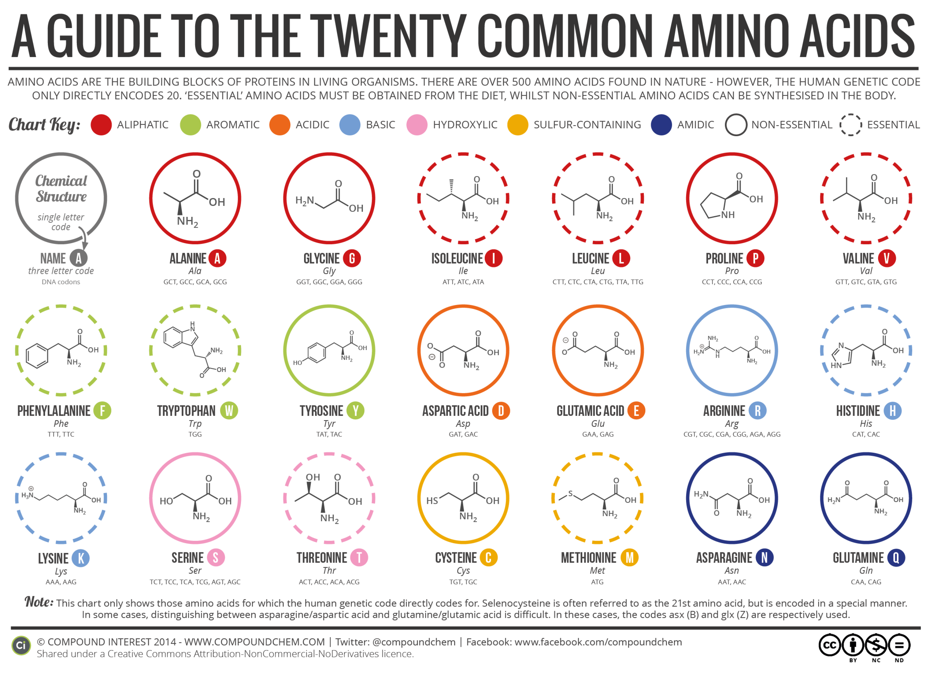
The suggested method involves constructing a database of Amino acid signatures for well-known attacks. There are 20 essential Amino acids (
Figure 1) in nature. Each Amino acid has a unique chemical structure that gives it specific properties [
3]. The Amino acid signatures represent encoded instances of network transactions using essential Amino acid labels that encode numerical structural properties using a Vigesimal numbering system to map ASCII codes to Amino acids. Then, a Neural Network model was created and trained on our Amino acids database, learning common patterns akin to attack signatures. This was achieved by capitalizing on similarities in Amino acid sequence structures and functional domain areas to cluster similar attacks. The end result is a trained model capable of identifying suspicious network transactions in real-time with minimal processing time and an acceptable false positive rate. The construction of this attack classification model encompasses the following steps:
Pre-process network transactions to prepare them for Amino acid mapping.
Map the processed data into Amino acids.
Generate structural properties for each Amino acid signature.
Train the deep classifier model using the training data subset.
Validate the correctness and accuracy of the model by applying it to the testing data subset.
The rest of the paper is organized as follows:
Section 2 delves into the related work, offering insights into prior research in the field.
Section 3, on the other hand, is dedicated to introducing the foundation of our study. It begins by presenting the source dataset (
Section 3.1) and describing the data preprocessing steps in
Section 3.2, followed by an exploration of Amino acid mapping (
Section 3.3). Additionally, the structural properties of Amino acid sequences are discussed in
Section 3.4.
The presented research methodology further encompasses the exploration of Neural Networks (
Section 3.5) and a thorough explanation of the deep learning model utilized (
Section 3.5.1). Furthermore, insights into the hyperparameters of the designed deep learning model are provided in
Section 3.5.2.
Section 4 showcases the outcomes of the experiments performed, while
Section 5 offers a comprehensive discussion of the results. In conclusion,
Section 6 summarizes the findings and outlines potential avenues for future research.
2. Related Work
Several research studies have proposed diverse Deoxyribonucleic-Acid (DNA)-encoding techniques, aiming to address various challenges in digital computing and network domains, particularly in the context of network intrusion detection. The genetic information within DNA is structured as a code formed by four chemical bases: adenine, cytosine, guanine, and thymine, denoted as A, C, G, and T. DNA encoding involves the conversion of regular text into a DNA sequence, which can further be translated into a representation of Amino acids.
Suyehira [
4] proposed an encoding and decoding algorithm tailored for a DNA-based data-storage system. The proposed encoding method offers a means to convert binary data into sequences that represent DNA strands. Importantly, this method takes into consideration the inherent biological limitations. The researcher introduced a mapping framework and translation process that translates hexadecimal data into codons, factoring in biological intricacies such as the exclusion of start codons, the prevention of repetitive nucleotides, and the avoidance of lengthy repetitive sequences. In this schema, each hexadecimal value is transmuted into a codon, which is a sequence of three nucleotides that encodes a specific Amino acid. This approach is inspired by nature, mirroring the way Ribonucleic Acid (RNA) strands are parsed by ribosomes in groups of three nucleotides. The use of hexadecimal characters grants the algorithm the versatility to encode various data forms, leveraging their binary representation. The researcher hypothesized that each hexadecimal character can be flexibly associated with one of several possible codon choices (randomly chosen). This innovation serves as a specific technique within the proposed encoding algorithm. In cases where the algorithm encounters difficulty in finding a valid codon to continue a sequence, a technique called backtracking is suggested. This involves reassigning a new codon for the previous hexadecimal character.
What sets this research apart is the novel DNA-encoding approach, characterized by two significant modifications. First, it employs hexadecimal representation instead of text. Second, the introduced mapping scheme takes into account biological constraints, which ultimately aiding in the subsequent translation process, guiding the conversion of codons into Amino acids.
Rashid [
5] introduced a method aimed at encoding various network packet attributes with utmost efficiency, using the fewest-possible characters. This method employs a four-character DNA-encoding strategy, referred to as DEM4all, which comprehensively represents all 41 attributes. The DEM4all-encoding technique utilizes four randomly chosen DNA characters to correspond to the complete spectrum of 96 potential values for network traffic attributes. The selection of four characters proves optimal for handling and symbolizing the full range of conceivable values. Importantly, due to its random nature, every execution generates distinct DNA sequences to depict each value. The choice of these four letters is strategic, as they have been carefully selected to encompass the widest range of attribute values. It is worth noting that the DNA representation is generated randomly during each execution, without drawing from any biological basis.
A new DNA encoding for misuse IDS based on the UNSW-NB15 dataset was proposed in [
6]. The proposed system is performed by building a DNA encoding for all values of 49 attributes. Then, attack keys (based on attack signatures) are extracted, and finally, the Raita algorithm is applied to classify records, as either attack or normal, based on the extracted keys. The Raita algorithm was published by Timo Raita in 1991. It is a string-searching algorithm that improves the performance of the Boyer–Moore–Horspool algorithm. Thus, for nominal attributes that have 151 unique values (corresponding to the total number of values of the protocol, service, and state attributes), four DNA characters are used that can handle all these values. For numerical attributes with 11 values (from 0 to 9 and a fraction point), two DNA characters are used, which can handle all these values to represent each digit separately. This paper used random DNA representations to encode the network packet attributes that have no biological basis.
Cho et al. [
7] delved into the potential adaptation and enhancement of a sequence-alignment technique prevalent in bioinformatics. The authors presented an advanced rendition of the Needleman–Wunsch algorithm, a tool for global sequence alignment, tailored to identify intrusions within the IoT landscape. This novel method incorporates a positional Weight Matrix to bolster its capabilities. A Weight Matrix is a strategy used to hunt for patterns within biological sequences. The assigned weights correspond to the frequency of occurrence of specific sequence elements in distinct positions.
Rashid et al. [
8] introduced two distinct DNA-encoding techniques known as DEM3sel and DEMdif, each possessing unique characteristics pertaining to the length of the DNA sequence and the manner in which network traffic is represented. Specifically, DEM3sel employs three characters to signify all 41 network attributes, while employing a single predetermined character to differentiate between nominal and numerical attributes. In contrast, DEMdif adopts diverse characters to represent network attributes based on their values and likewise utilizes a solitary pre-established character to distinguish between nominal and numerical attributes.
The study made use of the KDDCup’99 and NSL-KDD datasets, both of which are computer network traffic datasets. The attributes of the network traffic records were categorized into two groups: Nominal attributes (Protocol, Services, Flag) and Numerical attributes. Although both methods encompass fixed and dynamic elements, it is important to note that the choice of DNA representation is made randomly and is not guided by any biological reference.
Rashid et al. [
9] introduced a hybrid Network-Intrusion-Detection System (NIDS) that harnesses both DNA encoding and clustering techniques. In their proposed DNA encoding scheme, attributes from the UNSW-NB15 database (comprising network traffic records) are categorized into four groups: State, Protocol, Service, and Digits for the remaining attributes. The dataset encompasses various types of attacks and regular activities, with each entry comprising 49 features. These attributes are subsequently translated into DNA sequences via DNA encoding. Notably, each protocol attribute value is represented using a combination of four DNA elements. In contrast, the values of the State, Service, and Digit attributes are encoded using two DNA characters each. Following this encoding step, a clustering approach is employed to classify records into either attack or normal clusters. It is important to highlight that the chosen DNA sequences for attribute values exhibit varying sizes based on volume considerations and are tailored specifically without invoking biological references.
Cevallos et al. [
10] elucidated the steps involved in utilizing DNA as a storage medium, particularly focusing on the process of encoding digital information into DNA sequences. This process entails the conversion of a text file into a DNA sequence. The transformation happens in three distinct stages. Initially, each character in the text file is substituted with its corresponding ASCII value, subsequently represented in binary format. Finally, every two bits of the binary representation are further replaced by the corresponding DNA bases: A = 00, C = 01, G = 10, and T = 11. Furthermore, this study delved into the intricate relationship of nucleotide bonds within a biological context, providing a comprehensive mapping table that facilitates the encoding of Amino acids via binary representation.
In recent years, the field of bioinformatics has witnessed a shift towards utilizing Amino acid mapping in text encoding, departing from the more-traditional approach of DNA mapping [
11]. Several key advantages have emerged from this shift, demonstrating the effectiveness and versatility of Amino acid mapping in various applications.
Some advantages of Amino acid encoding over DNA encoding are as follows:
Increased information density: Amino acid mapping encodes text sequences with greater information density compared to DNA mapping. This is due to the fact that Amino acids achieve a more-compact representation than DNA encodings [
12].
Enhanced similarity measures: Amino acid mapping often results in improved similarity measures for text sequences. By preserving functional and structural similarities, it enables more-accurate comparisons between sequences, which is valuable in tasks such as sequence alignment and similarity searching [
13].
Robustness to mutations: Amino acid mapping is more robust to minor variations or mutations in text sequences. DNA mapping, on the other hand, can be highly sensitive to single-character changes, making Amino acid mapping a preferred choice in scenarios where text data may be noisy or subject to minor alterations [
14]. For example, proline is represented by four different codons (CCU, CCC, CCA, and CCG)
Compatibility with Amino acid sequence analysis tools: Amino acid mapping facilitates seamless integration with a wide range of bioinformatics tools designed for biological analysis. This compatibility enables researchers to leverage existing resources and tools in their text analysis tasks [
15].
Support for structural information: This can be particularly advantageous in applications since Amino acids are more relevant to biological processes than DNA nucleotides [
16]. DNA nucleotides are the building blocks of genes, but genes do not directly determine the structure and function of Amino acid sequences. The sequence of Amino acids determines its structure and function. This is the main reason to use Amino acid mapping in our research.
Reduced sequence length: Amino acid mapping often results in shorter encoded sequences compared to DNA mapping. This reduction in sequence length can lead to computational efficiency improvements in various text-processing tasks besides a reduction in the data storage needed [
17].
Alignment flexibility: Amino acid mapping allows for more flexible sequence alignments. It accommodates gapped alignments, which are essential in scenarios where text sequences may have insertions or deletions [
18].
These advantages collectively demonstrate the utility of Amino acid mapping in handling text sequences, making it a valuable choice in various bioinformatics and text analysis applications compared to DNA mapping. Those advantages have not yet been deployed for NIDSs, where DNA encoding was predominantly used. We, therefore, examine the use of Amino acid encoding for NIDSs in this paper.
3. Materials and Methods
The proposed Network-Intrusion-Detection System (NIDS) is divided into two phases: training and validation; production. Its implementation consists of four main steps: data preparation, feature generation, machine learning, and model evaluation and production.
Figure 2 shows the Network-Intrusion-Detection System (NIDS) in more detail. Initially, we under-sampled the UNSW-NB15 dataset. The next step was to extract features from the network traffic records based on the generated Amino acid signatures. The extracted features were then used to train a machine learning model. Once the machine learning model was trained, it was evaluated on a test dataset. The evaluation results (evaluation not shown in the diagram) were used to determine the accuracy of the model and to identify any areas where the model can be improved. The final step was to deploy the NIDS in the network.
3.1. Dataset
To devise an efficient technique for detecting network intrusions, it is crucial to have access to comprehensive and contemporary network flow datasets encompassing both regular and anomalous network traffic instances. These datasets should accurately represent real-world scenarios, focusing on pertinent attributes, to enable effective detection of network attacks. Such datasets should encompass diverse instances of attacks and intrusions encountered in network operations. However, a gap persists in the availability of authentic, up-to-date datasets that encompass the full spectrum of network traffic patterns associated with modern technology.
Traditional benchmark datasets like KDDCup’99 [
19] and NSL-KDD [
20] have been extensively utilized to assess the accuracy of network attack detection. However, these datasets have become outdated due to the swift evolution of network technologies and the emergence of novel cyber security threats and types of network attacks.
A network intrusion dataset comparison by Robertas et al. [
21] showed that UNSW-NB15 [
22] is one of the most-suitable datasets for our experiments. It is one of the most-recent datasets and has a large number of records with a variety of attack types compared to other datasets (
Table 1). UNSW-NB15 originates from the labs of the University of New South Wales (UNSW) Canberra, Australia. This dataset was generated utilizing the IXIA PerfectStorm tool within a confined network environment featuring only 45 unique IP addresses. The data span a concise period of 31 h and encompass a blend of both genuine typical activities and simulated attack behaviors, resulting in 175,341 training records and 82,332 testing records. The IXIA tool simulated nine diverse attack types. The dataset comprises 49 attributes available for analysis, encompassing fundamental features, content-related attributes (derived from packet content), time-based attributes (derived from time-related packet flow characteristics), and additional generated attributes based on statistical connection characteristics.
The choice of using classical datasets is primarily driven by their established reputation and widespread acceptance in the cybersecurity community. These datasets have been extensively used and validated in numerous studies, providing a benchmark for the comparison and evaluation of methods in this field. These datasets continue to be relevant due to the fundamental and timeless nature of the network behaviors they capture. They provide a diverse range of network traffic scenarios, including various types of attacks, which are still prevalent today. Moreover, the encoding of network data into Amino acid sequences is a novel approach. Applying this technique to these classical datasets allows new methods to demonstrate their effectiveness and versatility across different contexts and conditions. Using these well-known datasets (including UNSW-NB15) enables other researchers to replicate our experiments and validate the produced findings easily, promoting transparency and reproducibility in this research. We acknowledge that newer datasets could provide additional insights due to their reflection on recent attack techniques. However, for the scope of this paper, we believe that the chosen dataset sufficiently serves our research objectives.
3.2. Data Preprocessing
We employed the UNSW-NB15 DB dataset, which underwent a thorough examination by Moustafa [
22], as our labeled source for network transactions. Our particular focus rested on the disparity between attacks and normal instances. In this dataset, attacks constitute merely 13% of the records, while the remaining 87% are labeled as normal. This imbalance poses a challenge to the classifier model’s ability to generalize effectively during the training phase, particularly if we were to use the complete dataset. Furthermore, this imbalance could introduce a bias towards normal labels, consequently affecting the model’s predictive performance on unseen data.
First, we removed duplicate records, i.e., those having the same sequence. We ended up with nearly 100,000 attack-labeled records. Then, we under-sampled the normal transactions to have a 50/50 ratio with attack labels, producing a total of nearly 200k records.
Under-sampling is a technique that reduces the size of the majority class in an imbalanced dataset by randomly removing some of its examples. This can help to balance the class distribution and make the learning algorithm more sensitive to the minority class [
23,
24,
25].
The major advantages and disadvantages of subsampling are as follows:
Reduced computational complexity: Under-sampling can lead to reduced computational complexity, as it reduces the overall size of the dataset. Smaller datasets can be processed more efficiently, potentially resulting in faster model training and evaluation [
26,
27].
Improved model performance: Balancing the class distribution through under-sampling can lead to improved model performance, as it prevents the model from being biased towards the majority class. This can result in better classification accuracy and a more reliable evaluation of model performance [
24,
28].
Reduced over-fitting: Under-sampling can help reduce over-fitting (failure to generalize the model) in machine learning models. When a dataset is imbalanced, models may over-fit the majority class. Under-sampling the majority class helps prevent this issue, leading to models that generalize better to unseen data [
29].
Faster training: With a balanced dataset obtained through under-sampling, models often converge faster during training. This is because each class contributes an equal number of samples, allowing the model to learn from each class more effectively [
30].
Loss of information: Under-sampling can lead to a significant loss of information, as it involves removing instances from the dataset. This could potentially exclude important or relevant instances, leading to a model that is less accurate or representative.
Increased bias: While under-sampling can help address issues related to class imbalance, it can also introduce its own biases. Removing instances from the majority class could potentially bias the model towards the minority class. This could result in a model that performs poorly on new instances of the majority class.
To avoid model over-fitting, we need to split our modeling dataset (after under-sampling) into training and testing samples. The training part is used for model training and the testing part (unseen) to evaluate model performance. We split the dataset using the Holdout method by dividing it into 2 partitions with 80% for training and 20% for testing. We used K-fold Cross-Validation during the training phase of our classifier model to avoid over-fitting the model. Finally, we validated the correctness and accuracy of the model using the testing data. This was performed by comparing the generated labels from the model prediction method against the original ones.
As part of the data preprocessing, we standardized the dataset by centering each numerical value according to the mean and standard deviation of each feature column.
3.3. Amino Acid Mapping
Since our target domain had 20 Amino acids (as in
Table 2), we chose to use the Vigesimal numbering system as the intermediate mapping between ASCII representations of feature values and Amino acids. The Vigesimal system, also known as base-20, is a numeral system where the base is 20. This means that the system uses 20 distinct symbols (digits and letters) to represent numbers. In the Vigesimal system, the first 20 digits are represented as follows:
0, 1, 2, 3, 4, 5, 6, 7, 8, 9, A, B, C, D, E, F, G, H, I, J
In this system, after reaching digit 9, the symbol “A” represents the number 10, “B” represents 11, and so on, up to “J”, which represents the number 19. The number 20 is represented as “10” in Vigesimal, where “1” stands for 1 times 20 and “0” denotes 0 additional units.
As an example, the following counts from 1 to 30 in the Vigesimal system:
1, 2, 3, 4, 5, 6, 7, 8, 9, A, B, C, D, E, F, G, H, I, J, 10, 11, 12, 13, 14, 15, 16, 17, 18, 19, 1A, 1B
Table 2 shows the vigesimal values corresponding to each Amino acid.
The steps in the encoding process are as follows:
Replace missing values by NA;
Capitalize all letters (i.e., “tcp” “TCP”, “dns” “DNS”);
Convert each literal into its ASCII value (i.e., “A” 65);
Convert the ASCII value into its assigned Amino acid using the modulo 20 operation.
In
Table 3, examples of the process are given. Each step showcases the transformation of network-related data into a representation based on Amino acids, facilitating the comprehension of the encoding process samples of Amino acid encoding steps. Finally, all Amino acids resulting from one row of values will be appended in one sequence to represent the row Amino acid signature (
Table 4).
Each row within
Table 4 showcases the distinctive signature produced by concatenating the encoded Amino acid representations of the respective columns. From those examples, it is evident that the encoding process encapsulates the underlying patterns and characteristics of the input data in a condensed manner. This table, thus, exemplifies how the representation of data using Amino acids can yield succinct, yet information-rich signatures, enabling efficient and effective pattern recognition within network transactions. These artificial Amino acid sequences, while valuable for testing and research purposes, often differ from their natural counterparts. In
Table 5, we delve into the contrasts between these two types, exploring how our artificially generated Amino acid sequences differ from the intricate structures and functions of natural sequences.
Encoding network transactions into Amino acid sequences can greatly impact both the efficiency and effectiveness of analytical processes. Amino acids possess unique properties, enabling them to capture intricate patterns and relationships within data. They offer a highly compact and efficient way to represent data. Unlike traditional numerical values or binary encoding, which can be verbose and require significant storage space, Amino acid sequences provide a concise representation. By adjusting the encoding method that produces artificial Amino acid sequences, it can create sequences with similar structure and properties to natural Amino acids. Furthermore, it can be translated into DNA sequences, leveraging natural DNA’s exceptional data-storage capabilities, which also offers robust data security.
3.4. Feature Transformation: Structural Properties of Amino Acid Sequences
Most network transactional datasets have a large number of features to represent network and packet status [
31]. Since we have transformed the network data into an Amino acid sequence, we now use the Amino acid’s characteristics to describe the network data. In biology, different characteristics related to Amino acid structure are important in understanding their shape, function, and behavior. The structural properties of Amino acids are used as an analytical tool to understand how Amino acid sequences behave. Amino acids have a variety of features, including size, shape, and charge. These features affect how Amino acids interact with each other and how they fit together to change their structure. Some Amino acids are larger in shape than others, which affects how they fit together in a sequence. Amino acids also have different shapes such as curved, straight, or twisted. In addition, the charge of each Amino acid may be positive, negative, or neutral. Considering all these properties of Amino acids would give each sequencea unique identity to categorize it as attack or benign.
We can use these unique traits of Amino acids to identify potential issues or threats in network traffic. For example, if the Amino acid sequence of a network transaction has many twists (
turn value), it might be a sign of unusual network activity. Similarly, if the sequence has a specific Amino acid pattern (
strand value), it could be a sign of a known attack that has a similar and known sequence pattern. For each sequence of Amino acids, we calculated ten numerical structural properties that reveal different aspects of the Amino acid sequence structure and behavior. The structural properties of Amino acids reflect how the sequence folds, interacts, and performs its biological role. Using those properties is part of our contribution made by this research since it is a way to transform all network transactional features regardless of their variable count and data type into numerical features and still preserve the original data relationship through those transformed features. More information on how those features are calculated can be found in the ssbio documentation [
32]. The structural properties used were as follows:
turn: A
turn is like a U-turn in the Amino acid sequence structure that affects the sequence’s functionality. The
turn value is the percentage of Amino acids able to form that type of turn. It is calculated as:
where:
strand: A
strand is a pattern of the Amino acid sequence that is arranged in a flat, extended shape, almost like a ruler. The
strand value is the percentage of Amino acids able to form that type of strand. It is calculated as:
where:
Molecular weight: The molecular weight of the Amino acid sequence offers valuable clues about its dimensions and composition. The molecular weight has an impact on physical attributes and interactions. It is calculated as:
where:
Aromaticity: Aromaticity indicates the occurrence of aromatic Amino acids in the sequence. These aromatic building blocks play a role in maintaining Amino acid sequence stability and frequently engage in binding interactions. It is calculated as:
where:
q is the count of Amino acids in the sequence that are aromatic (the group of Amino acids that possess a characteristic ring-like structure like F, W, or Y).
n is the total number of Amino acids in the sequence.
Instability index: The instability index measures how prone an Amino acid sequence is to denaturation or clustering. A lower instability index indicates higher stability. It is calculated as:
where:
n is the total number of Amino acids in the sequence.
represents the ith Amino acid in the sequence.
instability_index_matrix is the instability value associated with the dipeptide (two Amino acids linked together by a molecular bond) formed by Amino acids in and
Isoelectric point: The isoelectric point corresponds to the pH where the Amino acid sequence holds no overall electrical charge. It is calculated as:
where:
f is the total number of ionizable groups in the sequence.
pKa = .
Ka is a measure of the strength of the Amino acid in a solution.
is the pKa value of the ith ionizable group.
The ionizable group in an Amino acid sequence refers to specific functional groups within the sequence that can either accept or donate their positive charge depending on the pH (level of acidity) of the surrounding environment.
helix: The helical characteristic signifies the abundance of
-helical structural components within an Amino acid sequence. Its value determines the percentage of certain Amino acids that are known to contribute to helical structures within Amino acid sequence. These Amino acids are “VIYFWL”. It is calculated as:
where:
m is the count of the Amino acids V, I, Y, F, W, and L in the sequence.
n is the total number of Amino acids in the sequence.
Reduced cysteines: This property evaluates the number of cysteine residues in the Amino acid sequence. It is also known as the molar extinction coefficient with reduced cysteines and is calculated as the weighted sum of the molar extinction coefficients of specific Amino acids in the sequence. It is calculated as:
where:
: percentage of the specified Amino acid in the sequence.
: molar extinction coefficient of the specified Amino acid. It measures how strongly the Amino acid interacts with light due to its unique chemical features.
Disulfide bridges: Disulfide bridges depict the chemical links established between pairs of cysteine residues, playing a role in stabilizing Amino acid sequence configurations, especially in extracellular surroundings. It is calculated as:
where:
N is the total number of cysteine residues in the Amino acid sequence.
is the distance between cysteine residue i and cysteine residue j.
(d) is a function that returns 1 if d is less than or equal to a threshold distance D (indicating that the cysteine residues are close enough to form a disulfide bond) and 0 otherwise.
GRAVY: The Grand Average of Hydropathy (GRAVY) index measures the general hydrophobic or hydrophilic character of Amino acid sequence.It is calculated as:
where:
These ten structural characteristics offer a multi-dimensional view of an Amino acid sequence.
Table 6 shows an example of this. Therefore, we converted the Amino acid representation into features using those ten characteristics. The following shows the role of each structural property in specifying information about sequence shape:
turn and strand capture the secondary structure of the Amino acid sequence, which is determined by the hydrogen bonding patterns between the backbone atoms. These properties indicate how the sequence bends and twists into different shapes, such as loops, coils, and sheets.
Molecular weight and aromaticity capture the size and composition of the Amino acid sequence, which affect its physical attributes and interactions. These properties indicate how heavy and complex the sequence is and how likely it is to contain aromatic rings that can participate in binding interactions.
Instability index and isoelectric point capture the stability and charge of the Amino acid sequence, which influence its solubility and denaturation. These properties indicate how prone the sequence is to unfold or aggregate and at which pH value it becomes neutral of charge. The pH value is a measure of how acidic or alkaline a substance is.
helix and reduced cysteines reveal important details about how the Amino acid sequence is shaped. It shows how often the sequence forms spiral-like structures, which influence the overall structure and stability of the Amino acid sequence.
Disulfide bridges and GRAVY capture the quaternary structure of the Amino acid sequence, which, with more bridges, can greatly influence the overall shape and stability. GRAVY gives us clues about whether the sequence prefers to stay in water. Both shed light on how much the Amino acid sequence is willing to react, changing its structure.
By using these 10 structural properties as the inputs for the Neural Network, we can represent the Amino acid sequence in a multi-dimensional space that captures its structural diversity and complexity. This can help us train the Neural Network on all result Amino acid structural properties values and predict the class of any new Amino acid sequence based on its structural properties.
We used BioPython [
33] and ssbio [
34] to calculate those structural properties. BioPython is a widely used Python library for bioinformatics and computational biology. It provides tools for parsing, analyzing, and manipulating biological data, including DNA and Amino acid sequences. ssbio is a Python package that provides a collection of structural systems biology tools. In our research, we used BioPython and ssbio as biological data analysis tools to calculate the structural properties of Amino acid sequences. This is an advantage because:
BioPython and ssbio are designed with a user-friendly interface, making them accessible to researchers with programming skills, but limited expertise in biology. This ease of use can facilitate collaboration between computer scientists and biologists.
BioPython and ssbio offer a robust and well-documented set of functions tailored to biological data analysis.
BioPython and ssbio also have modules for parsing and manipulating sequence data in addition to sequence structural analysis. These modules can help convert biological sequences into numerical values, which can be used as inputs for Neural Networks.
We can interpret the structural values in
Table 6 in the context of Amino acid sequence structure. A
turn value of 0.0 suggests that the sequence is unlikely to form this type of turn, suggesting the sequence may be more linear or may have other types of turns or structures. The absence of
turns could potentially affect the overall structure and functionality that this sequence forms.
The value 0.05 for strand indicates that the Amino acid sequence is 5% likely to form a strand structure. In simpler terms, a strand is like a flat, straight ribbon in the structure of an Amino acid sequence. It is one of the ways that the chain of Amino acids can fold and twist to form a biological structure. The value 0.05 suggests that there is a small chance that the sequence will form this flat, straight ribbon-like structure. In other words, most of the time, the sequence might prefer to fold and twist in other ways.
The molecular weight of the Amino acid sequence is 10,703.86, referring to the total weight of all Amino acids in that sequence. This gives us an idea about how many Amino acids are in the sequence and what types they are. Regarding aromaticity, each Amino acid can have different characteristics. Some are aliphatic, while others are aromatic, meaning they have a special structure that makes them stand out. A value of 0.15 for aromaticity means that about 15% of the Amino acids in our sequence are these special aromatic ones. Aromatic Amino acids help maintain the stability of their sequence structure and often participate in interactions with other molecules.
An Amino acid sequence with a high instability index (like 0.60 in this case) is more prone to changes or denaturation (the disruption or alteration of the natural shape and structure of the Amino acid sequence), which means it can easily lose its shape and function under certain conditions. The isoelectric point specifies the pH value at which the sequence has an equal number of positive and negative charges, making the Amino acid sequence overall electrically neutral. This could potentially affect how it interacts with negatively charged molecules or surfaces.
For the helix, the value of 0.26 suggests that about 26% of the Amino acids in our sequence are likely to be part of a spring-like coil shape. This is a significant portion and indicates the -helical structure is a key feature of this sequence. These coiled regions can help give the overall sequence structure shape and can also play an important role in its function, such as providing sites for other molecules to bind, which increases the change probability of the sequence. Reduced cysteines refers to the number of cysteine residues in our Amino acid sequence that are free and not engaged in bonds. A high value like 5210 (as in our case) means a high possibility for those free residues to engage in new bonds with other sequences and result in a major change in its sequence structure.
For disulfide bridges, the value 5960 means a high number of bridges in the Amino acid sequence, which likely contribute to a highly stable and rigid structure, as each bridge helps to lock the structure into a specific shape. A negative GRAVY score, like −1.82 in our case, indicates that the sequence is highly hydrophilic, meaning it has a high probability of interacting with water molecules by which its structure can be changed dramatically.
We applied this process to the whole preprocessed UNSW-NB15 DB dataset, replacing each network traffic record with the Amino acid sequence as in
Table 4, the ten numeric features as in
Table 6, and the attack label, which designates whether the transactions are normal or classified as attacks. This compilation constitutes our updated dataset.
Table 7 shows the steps for how to transform the original network transaction values into structural features using the BioPython and ssbio libraries to analyze the Amino acid sequence of each network transaction row.
3.5. Neural Network Learning Model
We designed a Feed-Forward Neural Network with the following topology: 10 input nodes, 1 hidden layer with 10 nodes, and 1 output node. The input features are the structural properties of the Amino acid sequences (
Table 6). Training and evaluation for each network took nearly 4 h.
Table 8 shows the Neural Network parameters used. The activation function, chosen as “Sigmoid”, introduces non-linearity, crucial for capturing intricate patterns. Employing the “binary cross-entropy” loss function quantifies prediction errors, aiding the model’s optimization during training. With 100 Epochs, the network undergoes iterative learning on the dataset. The Batch Size of 5 improves the efficiency by updating parameters in smaller subsets. These choices collectively enhance the Neural Network’s ability to accurately classify network transactions.
Our Neural Network architecture can be depicted as the composition of the input, hidden, and output layers, along with the respective number of nodes in each layer with the directed connectivity (
Figure 3).
The Neural Network design with one hidden layer in
Figure 3 is a simple example of a Feed-Forward Neural Network. It can be used to solve a variety of problems, such as classification, regression, and clustering. The Neural Network is trained by adjusting the weights of the connections between the neurons. The weights are adjusted so that the network minimizes the error between its predictions and the labels in the training data.
Data standardization techniques impact the performance of the experimental model (
Table 9). Each method’s effectiveness is measured by its resulting mean accuracy and standard deviation. During training, the Neural Network from
Figure 3, the first method, which does not involve any standardization, yielded a baseline accuracy of 55% with a standard deviation of 8%. In contrast, applying the “Standard Scaler” technique, which normalizes data by setting its mean to 0 and the standard deviation to 1, significantly improved the accuracy to 96.7% with a standard deviation of 6%. Similarly, the “Normal Scaler” approach, adjusting data to match the mean and standard deviation of its column values, achieved an accuracy of 96.9% with a smaller standard deviation of 1%. These results underscore the importance of data standardization in enhancing model accuracy and stability during the training process.
In order to make sure that a Neural Network is indeed the best choice for the problem [
35], taking into consideration the insufficiency of a training dataset challenge [
36], we examined a number of other machine learning techniques [
37]. Results for those are provided in
Supplementary Information (SI) Section S1.
3.5.1. Deep Learning Model
We added new hidden layers to our existing Neural Network to make it deeper and to enhance its data pattern recognition ability.
Table 10 shows the accuracies achieved with different numbers of hidden layers. For all Deep Neural Network experiments, we scaled the data using a Normal Scaler since it showed in previous Neural Network experiments the best accuracy among other Scalers.
Conducting multiple iterations of the same Neural Network while maintaining consistent input and output layers, as well as employing identical parameters (as shown in
Table 8), yet varying the configurations of the hidden layers, can yield diverse performance outcomes (
Table 10). “Deep Model 1” features a Neural Network structure with two hidden layers, each containing 10 and 5 nodes, respectively. This configuration achieved an average accuracy of 97.3% with a standard deviation of 30%, demonstrating a competitive performance. In contrast, “Deep Model 2” employs a more-complex architecture with four hidden layers (10 × 15 × 15 × 10 nodes). This increased depth and width resulted in a higher average accuracy of 98.3%, while the standard deviation dropped to 15%, showcasing improved stability. This table underscores the trade-off between network complexity and accuracy, highlighting how a deeper and wider architecture, as demonstrated by “Deep Model 2”, can lead to enhanced performance.
3.5.2. Hyperparameter Tuning
Neural Network hyperparameters are predetermined settings that are established prior to training a model and cannot be learned from the data themselves. These parameters play a pivotal role in shaping the model’s performance and its ability to generalize well. In light of the accuracy outcomes presented in
Table 10, we conducted experiments to fine-tune the hyperparameters for Deep Model 2.
To identify the optimal combination of hyperparameters that yields the highest accuracy, we employed hyperparameter-tuning techniques. Specifically, we used Grid Search, a mechanism that automates the process of systematically exploring various hyperparameter values from a predefined set. This exhaustive search allowed us to determine the configuration that best enhances the accuracy of Deep Model 2. The experimental hyperparameter ranges are shown in
Table 11. Detailed results for different numbers of folds can be found in
Supplementary Information (SI) Section S2.
The hyperparameters examined encompass the “No. of Folds in K-Fold Cross-Validation”, “Batch Size”, and “No. of Epochs”, each playing a significant role in influencing the model’s performance. Notably, the “No. of Folds in K-Fold Cross-Validation” reflects the number of subsets in which the training dataset is partitioned for training and validation. The model’s accuracy varies with different values of k, revealing how a more-comprehensive evaluation across varying subsets can lead to refined performance, as observed in the 20-fold validation, where the accuracy remarkably reached 99.0%.
The “Batch Size” and “No. of Epochs” parameters are crucial in guiding the model’s convergence and generalization capabilities. Higher “Batch Size” values tend to expedite convergence; yet, the experimentation showcased that values around 100 yielded favorable outcomes, indicating a balanced convergence rate while avoiding potential over-fitting. Similarly, “No. of Epochs” impacts the model’s ability to adapt to the dataset, with results indicating that an Epoch count of around 500 attains substantial accuracy without over-fitting concerns.
Furthermore, the effect of these hyperparameters became more-pronounced when considering the scale of the dataset. It is noteworthy that the results were measured on an under-sampled version of the UNSW-NB15 dataset with a 50/50 ratio of attack labels and a total of 200,000 records. This context underscores the model’s practical utility and potential for real-world applications. Overall, this comprehensive analysis of the experimental hyperparameters underlines their intricate interplay in enhancing the deep learning model’s accuracy and robustness in detecting network intrusion activities.
3.6. Software and Hardware
Our results were generated using Ubuntu 22.04.1 LTS (Jammy Jellyfish) running on and eight-core Linux machine with 11th Gen Intel(R) Core(TM) i9-11900K @ 3.50 GH and an Asus GeForce RTX 3090 ROG graphics card. Below, we provide an overview of the experimental development platform and tools used for conducting our research. These tools and libraries were instrumental in the successful execution of our experiments, ensuring the accuracy and reliability of our results.
Experimental development platform:
Python: Version 3.7.15;
Integrated Development Environment (IDE): Spyder Version 5.3.3;
Database: SQLite Version 3.40;
Dataset: UNSW-NB15 dataset files were used in Excel format.
Python development platform:
External libraries:
BioPython: Version 1.77;
scikit-learn (sklearn) [
39]: Version 1.3;
Keras: Version 2.6;
TensorFlow: Version 2.6.
4. Results
Table 12 provides a summary of key performance metrics for our Neural Network model’s performance in classifying between benign (0) and attack (1) instances during the validation phase using the testing data, which were 20% of the total data. It shows that the model achieved a good precision, recall, and F1-Score for both classes, with an overall accuracy of 97%, a precision of 98%, a recall of 97%, and an F1-Score of 97%. We used 199,286 data rows in total, with a 50/50 ratio between the benign and attack rows and an 80% training/20% testing ratio. The weighted average for the precision, recall, and F1-Score was 97%.
Table 13 provides a comprehensive overview of the performance metrics, including the precision, recall, F1-Score, support, accuracy, macro-average, and weighted average, used to evaluate the effectiveness of the model across different classes and overall accuracy.
Table 14 shows the counts from the confusion matrix. There were 97,308 instances (97.77%) that were correctly predicted as benign (true negatives), 2335 instances (2.34%) that were benign, but were incorrectly predicted as an attack (false positives), 3039 instances (2.43%) that represented attacks, but were incorrectly predicted as benign (false negatives), and 96,604 instances (97.63%) that were correctly predicted as attacks (true positives).
The best results using the deep classifier model that we defined in
Table 10, using different settings for the hyperparameters from
Table 11, are reported in
Table 15. The best accuracy was 99%, with Batch Size = 100 and No. of Epochs = 500. With this combination of hyperparameters, the standard deviation of the accuracy was 27%. The other combinations of hyperparameters achieved mean accuracies ranging from 98.84% to 98.95% with standard deviations ranging from 17% to 37%. The lowest mean accuracy of 98.84% was achieved with a 10-fold cross-validation, a Batch Size of 200, and 500 Epochs. With this combination of hyperparameters, the standard deviation of the accuracy was 23%.
In general, a higher accuracy was achieved with a larger Batch Size and a higher No. of Epochs. This is because a larger Batch Size allows the model to learn more from each training iteration, and a higher No. of Epochs allows the model to train for a longer period of time. However, there is a point of diminishing returns where increasing the Batch Size or the No. of Epochs does not significantly improve the accuracy of the model. This is because the model can only learn so much from the data, and after a certain point, the additional training will not yield any significant improvement. The relationship between the accuracy and hyperparameters can vary depending on the specific dataset and the model architecture. This is because different datasets and model architectures have different characteristics, which can affect the optimal hyperparameter settings.
The highest accuracy of 99.0% was achieved with a Batch Size of 100 and 500 Epochs. This suggests that these hyperparameter settings are optimal for the Deep Model 2 architecture and the dataset used in this experiment. The accuracy was still relatively high (98.9%) with a Batch Size of 50 and 500 Epochs. This suggests that a smaller Batch Size can still be effective if the No. of Epochs is increased. The accuracy decreased slightly with a Batch Size of 200 and 500 Epochs. This suggests that a larger Batch Size may not be necessary for the Deep Model 2 architecture and the dataset used in this experiment.


