Abstract
In the context of long-term infectious disease epidemics, guaranteeing the dispatch of materials is important to emergency management. The epidemic situation is constantly changing; it is necessary to build a reasonable mechanism to dispatch emergency resources and materials to meet demand. First, to evaluate the unpredictability of demand during an epidemic, gray prediction is inserted into the proposed model, named the Multi-catalog Schedule Considering Costs and Requirements Under Uncertainty, to meet the material scheduling target. The model uses the gray prediction method based on pre-epidemic data to forecast the possible material demand when the disease appears. With the help of the forecast results, the model is able to achieve cross-regional material scheduling. The key objective of material scheduling is, of course, to reach a balance between the cost and the material support rate. In order to fulfil this important requirement, a multi-objective function, which aims to minimize costs and maximize the material support rate, is constructed. Then, an ant colony algorithm, suitable for time and region problems, is employed to provide a solution to the constructed function. Finally, the validity of the model is verified via a case study. The results show that the model can coordinate and deploy a variety of materials from multiple sources according to changes in an epidemic situation and provide reliable support in decisions regarding the dynamic dispatch of emergency materials during an epidemic period.
1. Introduction
COVID-19 is a severe global public health emergency that has had a profound impact on medical systems and social economies [1]. During the outbreak of large-scale infectious diseases, the scheduling of emergency supplies is necessary to ensure medical treatment and the continuation of normal life. Thus, it is important to establish an emergency resources supply system fully tailored to the epidemic process. Among the issues linked with emergencies, methods of efficiently dispatching resources require attention. There are many factors affecting dispatching, including external factors, such as region and time, and internal factors, such as material supply and demand. A state of uncertainty and emergency increases the difficulty of dispatching materials. Therefore, the first factor that must be considered is the prediction of the possible demand through scientific methods. A two-stage location-routing model has been proposed for guiding resource allocation when the requirements and infrastructure are unknown [2]. The model has a lower computational cost because of its simple calculation process. Then, case-based reasoning (CBR) and the Dempster–Shafer theory have been employed to improve the accuracy in forecasting emergency material demand [3]. A good method is necessary not only for estimating demand but also for the organization of the supply chain and the coordination of the relationship between the parties in order to enhance the effectiveness of the material distribution. A two-stage MADA-B mechanism was designed to research the supply and demand of multi-attribute emergency materials, which combines a multi-attribute double auction (MADA) with bargaining and can perfectly match buyers with sellers through the game playing of the transaction price and quantity [4]. After demand matching is completed, the subsequent production plan becomes the new focus. Then, a fuzzy linear programming model was provided to solve the aggregate production planning problem. Its advantage is the incorporation of uncertainty of the customer demands, and unit holding and backordering costs of the production plan [5]. In one work, a method based on the timed-colored Petri net (TCPN) model was proposed to model the cooperation of actions with time analysis [6]. After the production of materials, timeliness needs to be considered in the selection of transportation methods. After an in-depth discussion of the cold chain model selection problem, taking into account economic and environmental objectives from both business and financial aspects, a value-based management method is provided as a new shipping approach [7]. The method effectively solves material planning by cutting out unnecessary actions. Other methods focus on the quick construction of the supply chain according to the criterion of reaction speed. Based on this idea, a hybrid algorithm combining artificial immunity with ant colony optimization has been developed, the transportation scheme of which has a shorter response time and covers more demand points [8]. With the hierarchical timed color Petri net (HTCPN) model and the skyline operator, a multi-objective optimization (MOO) model for a fire emergency response was established, which not only shortened the response time but also reduced resource consumption [9]. It must be noted that the above methods assume that materials are directly transported from the supply side to the demand side. They do not take into account cross-regional transportation, which is more likely in epidemic situations. To overcome this disadvantage, an inter-regional emergency cooperation network that includes system construction, organization and coordination, and mechanism design is proposed to offer an optimal countermeasure for city cooperation [10]. Transit points need to be considered when cross-regional issues are involved. The location of transit points will affect transportation efficiency. Considering this, a multi-objective optimization model for the selection of rescue stations has been established to improve efficiency [11]. In the research into transit points for cross-regional issues, the requirement for warehouses becomes obvious because it is nearly impossible to match the rate of supply with the rate of consumption. A mixed-integer programming model for uncertain requirements controlled by time and cost provides a helpful solution for emergency warehouse location and distribution [12]. Additionally, when stocks are available, a simulation–optimization approach based on the stochastic counterpart or sample path has been shown to optimize the pharmaceutical supply chain by managing the records of the stocks [13]. Due to the uncertainty of epidemics and the timeliness of drugs, medical demand is difficult to predict and handle. For that, a deterministic MILP model and a robust optimization model are used to deal with the demand uncertainty while integrating warehouse selection, inventory strategy and delivery route optimization of the VMI [14].
The above examples from the literature show different solutions for emergency events. However, all of them ignore the fact that the degrees of urgency of different requirements play a role in the response, especially when the emergency supplies are not enough to meet all of the requirements. In this situation, the distribution of materials has to consider the degree of urgency. An optimization model combines the location hazard index (LHI) with the response time; the LHI measures the potential hazard of a location, while the response time provides resource allocation in response to an emergency situation [15]. From the observation of multiple independent emergency events, a deep ensemble multitask model integrating four subnetworks has been proposed. It can improve the medical dispatch process by classifying the degree of emergency based on clinical data, environmental data and other factors [16]. In the case of an epidemic outbreak, a hybrid multi-verse optimizer algorithm based on the multi-verse optimization algorithm and the differential evolution algorithm can effectively reduce the distribution cost by considering the urgency of the demand for emergency supplies [17]. Numerous studies have comprehensively discussed good solutions for dispatching materials by recreating the scene of the emergency. The pre-emergency warning process has become another research hotspot. A study has formulated a multi-objective mixed-integer non-linear programming model to determine the location and number of relief centers, with their prepositioned inventory level, in the pre-emergency stage. The decision provided by the model can minimize costs and transportation distances [18].
The above literature examples discuss the various factors that support a reasonable resource-scheduling solution to advance the development of emergency management. However, most of the studies concentrate on static analysis to optimize resource scheduling, which means that the variations in the requirements and degrees of emergency are totally ignored in the process. In addition, the works mainly focus on the post-stage response, and the pre-stage early warning mechanism is rarely involved. In order to offer a solution incorporating all factors, a coordinated allocation model of multiple materials based on the gray prediction model is proposed in this work and is named the Multi-catalog Schedule Considering Costs and Requirements Under Uncertainty. If the number of infectious members of the population can be forecast, then the materials that will subsequently be required can be prepared. Thus, by collecting information on historical infectious diseases, the model uses a gray prediction algorithm to predict the number of infectious diseases in the future. According to the prediction results, the demand relative to infectious disease is determined, and this includes both medical materials and general goods. At the same time, the cost is also considered. With the goal of reducing the cost and meeting demand, a multi-object function is defined and takes into consideration the type of relief material, the time difference, and trans-regional coordination. This model contains numerous variables from different angles, meaning it is difficult to set the initial solutions. The ant colony model does not require much for the initial solutions and has few parameters, meaning that it is suitable for combinational optimization problems such as material dispatch. Therefore, an ant colony model is designed to solve our problem. The contributions of this work are as follows:
(1) The gray prediction algorithm is used to predict the number of confirmed cases at various times. Then, the degree of emergency can be estimated, and the predicted data can be used to guide material scheduling. The application of this prediction module means that our model can play a certain role in early warning systems.
(2) Both external and internal factors are considered in order to expand the scope of the model’s application and improve the satisfaction of the solution provided by the proposed model. External factors include distances and the time of transportation. The internal factor comprises the maximum level of production. Then, an objective function for cross-regional scheduling is defined, in which the uncertainty of requirements and different types of goods in a period of time are taken into account.
(3) In order to obtain the final schedule, the model uses the ant colony algorithm to solve the objective function. There are numerous integer variables in the function, and the initial solution is a three-dimensional matrix. Thus, the model records the directions of each ant’s action in each dimension in the matrix and defines a utility function, which is used to calculate the effect of the ant’s every choice. Unlike the pheromone, the calculated results will help shorten the time required to obtain the result of the model by adjusting the probability of picking the direction in the course of each ant’s actions.
This paper consists of five sections. Section 1 mainly describes the latest achievements regarding the research issues in this paper and discusses their advantages and disadvantages. Then, the model and the research value proposed in this paper are briefly introduced. Section 2 provides a detailed introduction to the theories used in the model. Section 3 consists of the building and solving processes of the model. The results of the model are verified and presented using examples in Section 4. Finally, the conclusions are discussed in Section 5.
2. Preliminaries
2.1. Gray Prediction
The gray prediction method GM(1,1) is a prediction system that can contain both known and unknown information. Based on the rule of data change, it generates a sequence with strong regularity and then the corresponding differential equation is built to predict the developed values of the data. Compared with other prediction methods, the gray prediction model only needs a few samples to drive, which is suitable to deal with the emergency because emergency always happens in a short time, and it is hard to gather enough observations during it. Therefore, in this paper, the gray prediction model is used to complete the prediction job [19]. The model is defined as follows [20].
We assume that the reference data column is , whose 1-AGO is as follows:
Formula (1) is the accumulating generation operator (1-AGO) of the reference data column, and it is obtained via Formula (2). In Formula (2), . is the number of observations. The mean generated sequence of is , where :
The gray differential equation is established:
In Formula (5), are the parameters of the equation. The values of are calculated by the immediate mean of the original data series. It is worth noting that when performing the immediate mean calculation, since the first data point does not have the previous data point, it needs to be averaged with the second data point. The whitening differential equation corresponding to Formula (5) is as follows:
According to least squares, the estimated value of for minimizing is obtained as . To solve the whitening differential equation, the formula is as follows:
The model accuracy is mainly verified using three items: a residual test, a correlation test, and a posterior error test. The residual test refers to the point-by-point comparison of the residual difference between the calculated value and the actual value. First, we calculate according to the method. Then, the predicted value of the original sequence is calculated according to Formula (11).
The absolute residual sequence is formed from the results of Formulas (11) and (12). The relative residual sequence is formed from the results of Formula (13). Then, the average relative residual is shown in Formula (14). For the given , the model can be regarded as qualified when and are both true.
The correlation degree test refers to the comparison of the similarities between the computed sequence curves and real sequence curves. The correlation coefficient is defined as Formula (17):
is the absolute error of sequence and at point. represents the minimum distance between the corresponding points in sequence and when remains the same. aims to traverse to find the minimum value in the result of . The calculation process of is the same as , except that is looking for the maximum. is the resolution. Usually, when and where , the model is considered as qualified.
The posteriori error test refers to testing the statistical characteristics of the residual distribution. A series of statistical indicators needs to be calculated. The following Formula (18) is the average of the original sequence. Formula (19) is the standard deviation of the original sequence. Formula (20) is the mean of the residual. Formula (21) is the standard deviation of the residual:
Calculate the variance ratio: . is the variance calculated from the original sequence . is the variance calculated from the residual sequence . Calculate the small residual probability: . Generally, when and , the model is acceptable.
2.2. Ant Colony Algorithm
The ant colony algorithm is an intelligent optimization algorithm. The basic ACO model is described by the following three formulas [21]:
In the ant colony algorithm, an ant chooses the next destination at each iteration until it has completed its journey. For example, at iteration , the ant moves from to . belongs to the set for the feasible location. is the probability that the ant will go from to at time . The heuristic values , where is the distance between and . The amount of pheromone trail maintained at the connection between and represents the learned desirability of choosing when at point. is the pheromone concentration on the to route in the next time period. It is calculated via the addition of the heuristic values and the experience acquired by the ants. The possibility of this step follows Formula (22), where and are positive constants. The pheromone trail on the path from to is updated as Formula (23) where is the pheromone evaporation coefficient expressed by a constant within interval and is the total number of ants. is the pheromone trail deposited by ant as in Formula (24). is the length of the tour taken by ant at step . If ant does not go from to at time , then the pheromone left by ant along this path is 0.
3. Problem Description and Optimal Model
3.1. Problem Description
Due to the large number of viruses and the constant emergence of new variants, epidemic outbreaks have the characteristic of being sudden and uncertain. According to the scale of the epidemic, it can be divided into two stages: a stable period and an outbreak period [22]. As shown in Figure 1, the number of cases increased significantly in April 2022; the data for this period are about nine times higher than those for March 2022 and about fourteen times higher than those for April 2021. Then, the number of cases fall back to the normal range in May 2022. Therefore, April 2022 can be classified as the outbreak period. The remaining months are classified as stable.
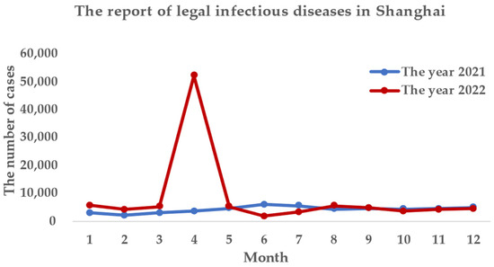
Figure 1.
The report of legal infectious diseases in Shanghai.
The difference in the data in April between the two years is very large in Figure 1, which verifies the uncertainty feature of the outbreak. Because of the uncertainty of the outbreak, the additional demand for resources with an outbreak is difficult to estimate. For example, in order to solve the problem of material distribution during the peak in April 2022, an e-commerce platform first added 3246 couriers to Shanghai. However, it was found that the increase in staff was not enough. Then, another 1754 staff members were reassigned to Shanghai. It can be seen that the uncertain requirements and the dynamic situation of the epidemic are the main difficulties in resource allocation.
This paper focuses on solving the problem by coordinating the dispatch of various anti-epidemic materials in multiple regions and multiple periods, considering the changes in the emergency situation and the premise of uncertain demand.
3.2. Model Building
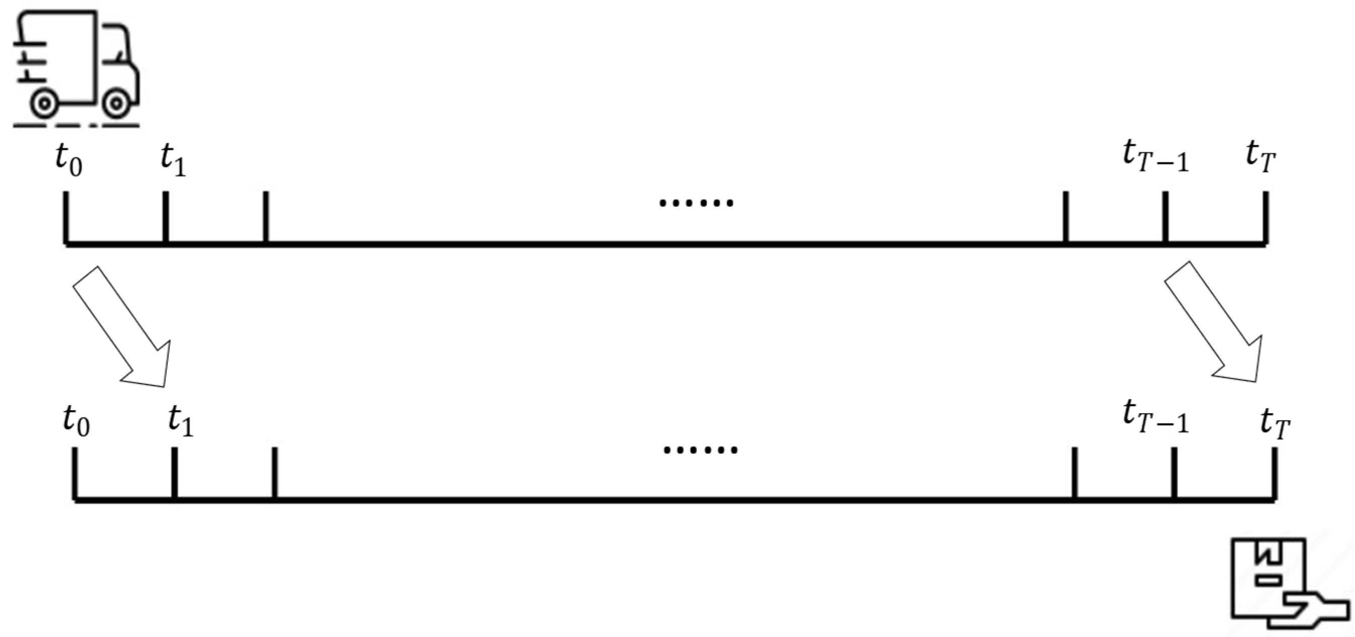
The following assumptions are made for the model: (1) There are three parties involved in the emergency supply system, including responsible organizations in the epidemic areas, suppliers of class A resources and suppliers of class B resources. (2) Three types of supplies—daily necessities, medical supplies and testing materials—are needed. Class A suppliers can provide daily necessities and testing materials; class B suppliers can provide medical supplies and daily necessities. (3) The threshold of requirements is set as %, which means that at least % of materials on the demand list must be met. (4) The production cycle of the suppliers is a unit time , and the entire epidemic period is . The process from producing goods to delivering them is shown in Figure 2, and the time difference between the production of a resource and its delivery is shown in Figure 3. The model parameters are shown in Table 1.
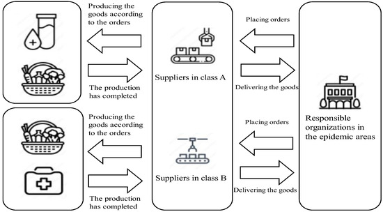
Figure 2.
The process between the production of goods and their delivery.

Figure 3.
The time between the production of a resource and its delivery.

Table 1.
Model parameters’ definition.
The responsible organizations in the epidemic areas issue detailed information to the suppliers cataloged into A and B in stages according to the material demand according to type and quantity. The suppliers produce and transport the materials based on the orders, and the organizations pay the bill when the materials are delivered. The costs are computed as follows:
There are two situations that can arise in the process of material supply, namely material shortage and material oversupply. The shortage of materials is not conducive to the implementation of emergency measures, while the oversupply of materials will generate carrying costs. The penalty cost is employed to describe the impact of these two scenarios and is calculated as follows:
A good solution should be generated via the selection of suitable suppliers to meet requirements at a low cost. Based on this idea, the objective functions are defined as follows:
Formulas (34)–(37) indicate the amount of materials transported by category A and B suppliers. They suggest that the amount of all the materials should not exceed their own production capacity. Formulas (38)–(40) indicate that all the materials transported by the suppliers in category A and B should meet at least of the needs of the epidemic area. Formula (41) indicates the decision variables by which materials are produced by class A and B suppliers.
3.3. Model Analysis
First, the model is built to achieve the goal of reducing costs while meeting material requirements. The cost is represented by money, an entity whose value as a commodity is equal to its value as money. Thus, the numerical value of currency can represent the value of goods [23]. However, this is a very complex problem that needs to consider both economic factors and living security. With a limited budget, it is helpful to consider economic factors, and living security is crucial. Therefore, two objective functions and are respectively defined to minimize the cost and the difference between of supply quantity and the required quantity. To sum up, the problem studied in this paper is still an optimization problem in essence. In order to solve it, there are two main ways to build the framework of the model: one is called predict-then-optimize, and the other is called Smart “Predict, then Optimize” (SPO) [24]. These two modes have different focuses on prediction. Predict-then-Optimize attaches great importance to the accuracy of prediction, while SPO pays more attention to the bias cost of decisions in similar situations. Considering that the prediction part of the paper aims at material demand, the accurate matching of material demand and supply is one of the most important requirements in the rescue process, so this paper chose the predict-then-optimize framework to establish the model.
Second, the number of confirmed cases, denoted as , is a dynamic variable affected by time; as a sequenced result, the amount of various emergency materials expressed as are also changed. This improves the uncertainty and increases the difficulty of this problem. In this work, the number of confirmed cases at time is set as the first parameter affecting others because the requirement for supplies at a given time in the epidemic area is mainly affected by the number of infected people [25]. Formula (42) is the prediction formula where is the result of the gray prediction model. To obtain the value of , the number of confirmed patients in periods before time is taken as the input for the gray prediction method, which is used to predict the possible number of confirmed patients at the following times. Adjusting can change the input number of variables in the gray prediction model so as to adjust the prediction results. The specific adjustment analysis is discussed in the subsequent experiment. Then, the material requirement is obtained by converting the predicted results through Formulas (43)–(45). , and are determined by . , and are respectively the demand coefficients of the three types of materials.
The model randomly generates several groups of feasible solutions and uses the ant colony algorithm to optimize each group of feasible solutions. Finally, we compare the optimization results to obtain the resource procurement allocation scheme. The original ant colony algorithm mentioned above relies on the experience of all ants to drive. This method is limited to high-dimensional problems because the large solution space weakens the effect of the rule of thumb of ants. Therefore, for high-dimensional problems, randomness is added to help expand the search scope of the solution while considering the experience accumulation of ants [26]. Inspired by this, this paper proposes an alternative treatment to help ants explore the solution space. The process of optimizing feasible solutions is as follows. In the optimization process, the model aims to achieve lower costs by changing the transportation schedule at time . So, at time , the model sets as the transport matrix, and represents the amount of materials transported by supplier to responsible organization , which is also the number of orders issued by responsible organization to supplier . The difference between the transportation volume before adjustment and the volume after is . The adjustment directions are divided into three categories: increase, decrease and unchanged. is set as the transportation volume at time after adjustment, and its relationship with is shown in Formula (46).
denotes the direction of adjustment, which belongs to . is the set of at time . If we assume is the set of all the directions that the ant can choose, then belongs to . The initial solution should be able to explain the origin and the end of the transportation and the transportation volumes at any moment, meaning that it should be a three-dimensional matrix. In the original ant colony algorithm, each iteration indicates that each ant has finished its journey. For this model, it signifies that every in the solution has changed, where . However, there are so many variables that it is hard for the model to obtain the final scheme, even with the help of the remaining pheromone trail. Therefore, this paper sets another utility function to lead an ant to reach its destination faster. Formulas (48)–(55) explain the mechanism of the utility function.
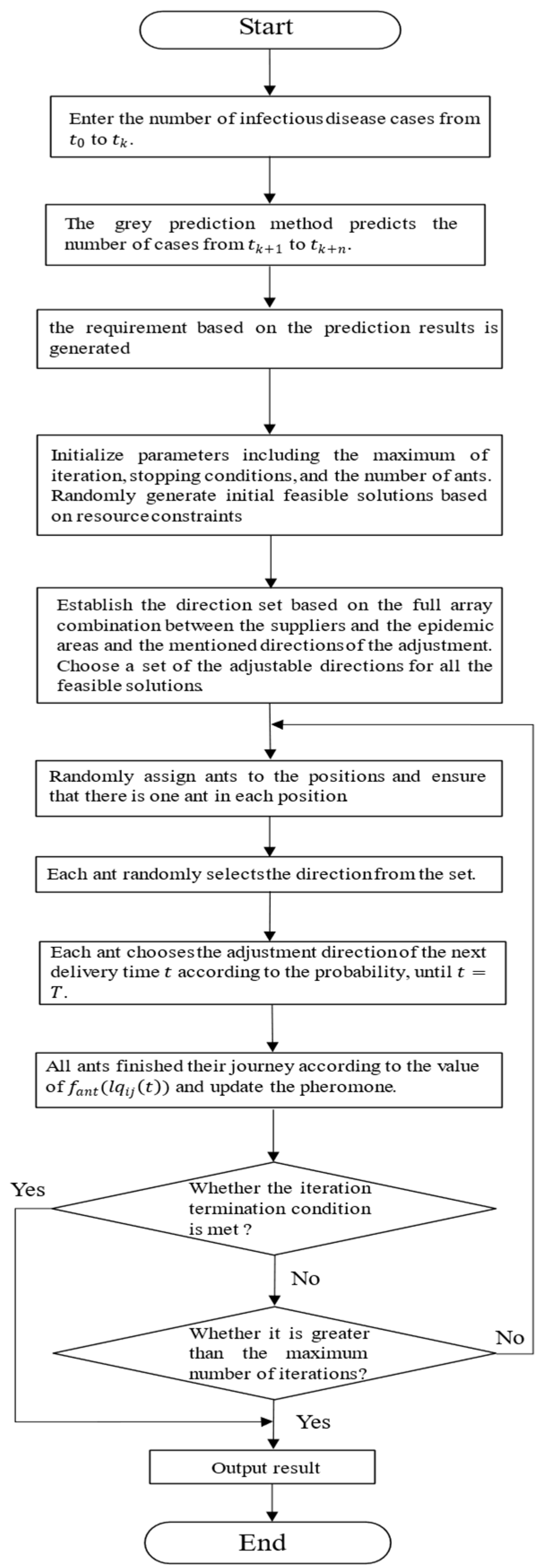
If the chooses the direction at time , then . is the utility function that consists of and . are used to adjust the weight. is the difference in the transportation volume before and after the change at time . represents the effect of making this change. is the probability of choosing direction at time . At the same time, the probability of picking the other directions decrease equally as Formula (52). represents the number of iterations of the optimization process. Then, as in Formulas (53)–(55), after all ants have finished their journey, they exchange experiences and then move on to the next iteration. The solution process for the algorithm is shown in Figure 4.

Figure 4.
Flow chart of the MS-CR-U.
Now, the complete model named the Multi-catalog Schedule Considering Costs and Requirements Under Uncertainty (MS-CR-U) has been introduced. First, the uncertainty caused by the dynamic characteristics of epidemics is measured through the gray prediction method. A multi-catalog model means that the types of materials and catalogs of suppliers are both partitioned because most of the suppliers focus on fixed goods. The production ability, cost and requirements are taken into the objective functions defined by the model to improve the application. Finally, the ant colony algorithm is employed to provide the solution for the model. The details of the model designed based on the ant colony algorithm are as follows:
- Step 1: Enter the number of infectious disease cases from to .
- Step 2: After the gray prediction method predicts the number of cases from to , the requirement based on the prediction results is generated according to Formulas (42)–(45).
- Step 3: Initialize parameters, including the maximum iterations, stopping conditions and the number of ants. Randomly generate initial feasible solutions based on resource constraints according to Formulas (34)–(41).
- Step 4: Establish the direction set based on the full array combination between the suppliers and the epidemic areas and the mentioned directions of the adjustment. Choose a set of adjustable directions for all feasible solutions.
- Step 5: Randomly assign ants to the positions and ensure that there is one ant in each position.
- Step 6: Each ant randomly selects the direction from the set.
- Step 7: Each ant chooses the adjustment direction of the next delivery time according to the Formulas (50)–(52), until .
- Step 8: All ants finish their journey and update the pheromone according to the Formulas (53)–(55).
- Step 9: Check the stopping criterion. If yes, go to Step 11; otherwise, go to Step 10.
- Step 10: Check whether the upper limit is reached. If yes, continue; otherwise, go to Step 5.
- Step 11: Output the result.
4. Data Analysis and Prediction Results
The problem solved using the MS-CR-U is to build a complete method for coordinating and dispatching multiple anti-epidemic materials under the condition of varied requirements during the epidemic period. In order to foresee possible situations, the number of historical infectious disease cases is used to sum up past experience. Additionally, it should be noted that climate is an important factor affecting the occurrence and spread of infectious diseases [27]. Thus, the mean temperature and precipitation data from 2020 to 2022 for 34 cities are shown in Figure 5. After observing the data, three types of characteristic climate items can be described, which are called the south type, north type and north–south junction. As the spread of infectious diseases is also related to the population size, in order to control the variables, this paper selects three cities with similar population sizes from the three climate types to collect statistics for infectious diseases. The data came from the websites of the health commissions of the three cities. As the date of the earliest data in the three cities is not consistent, the data from January 2018 to August 2022 are uniformly utilized for collation.
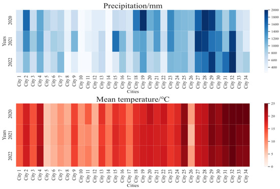
Figure 5.
Heat map of precipitation and average temperature.
4.1. Data Analysis
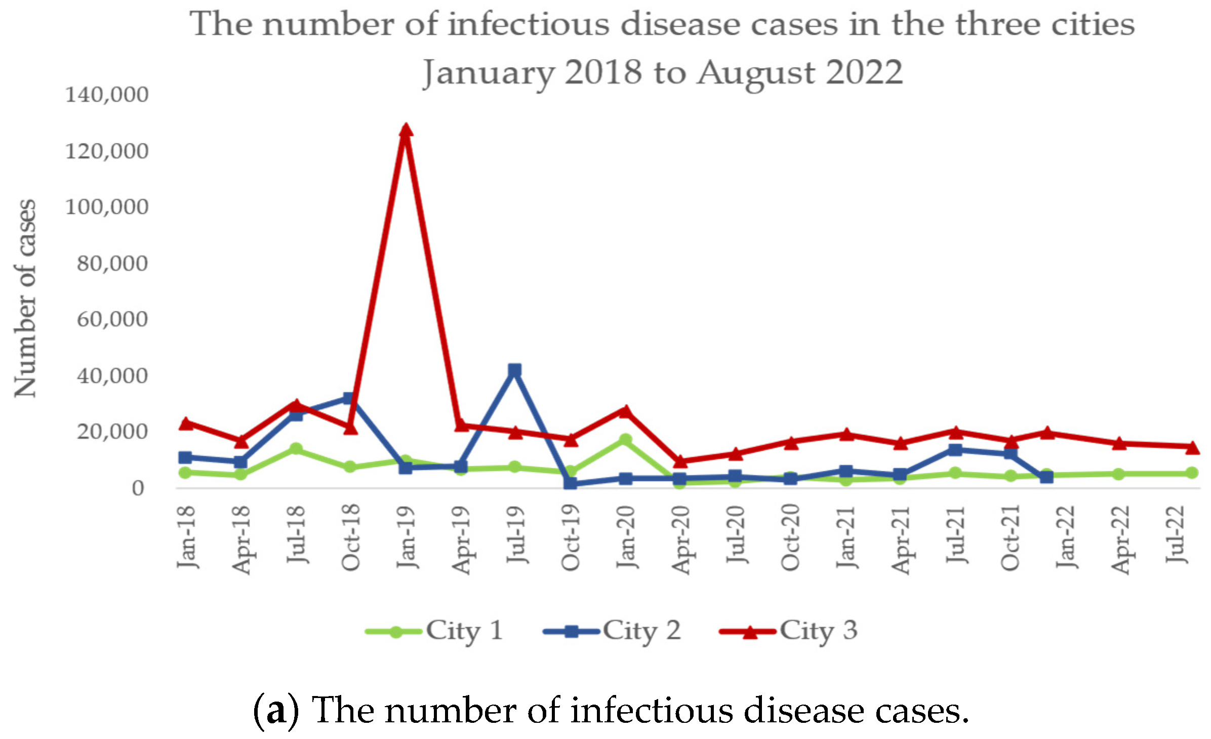
As shown in Figure 6a, in January 2019, there was a peak in the outbreak of infectious diseases in City 3. Within one month, the growth rate of infectious disease was as high as 425.5%. According to a public report, from December 2018 to January 2019, the temperatures of City 3 dropped significantly. In early December 2018, the temperature in City 3 remained around 10 to 20 degrees, but in early January 2019, the temperature dropped to −1 to 5 degrees. Within a month, the average temperature dropped by 52.25% and the Air Quality Index (AQI) increased by 19.15%. Based on the situation that climate change is predicted to increase the frequency and intensity of extreme weather events, amplifying air pollution levels and exacerbating respiratory diseases [28], and many people were infected with influence because they could not adapt to the temperature change. That is why the number of cases in City 3 soared within a month. Between the end of 2019 and the beginning of 2020, there was a small peak in Cities 2 and 3. Due to a series of epidemic prevention measures taken after the outbreak, the total number of infectious diseases in the three cities decreased by 57.7% in 2020. People adopted the habit of wearing masks, which effectively limited the spread of infectious diseases. During 2022, the number of cases in Cities 2 and 3 increased slightly at different time points. On account of the continuous mutations in the novel coronavirus in the process of transmission, the spread of new strains led to repeated outbreaks.
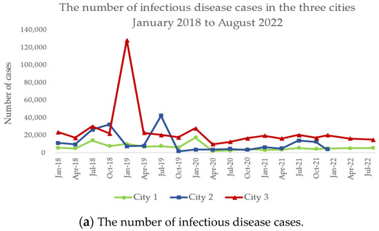

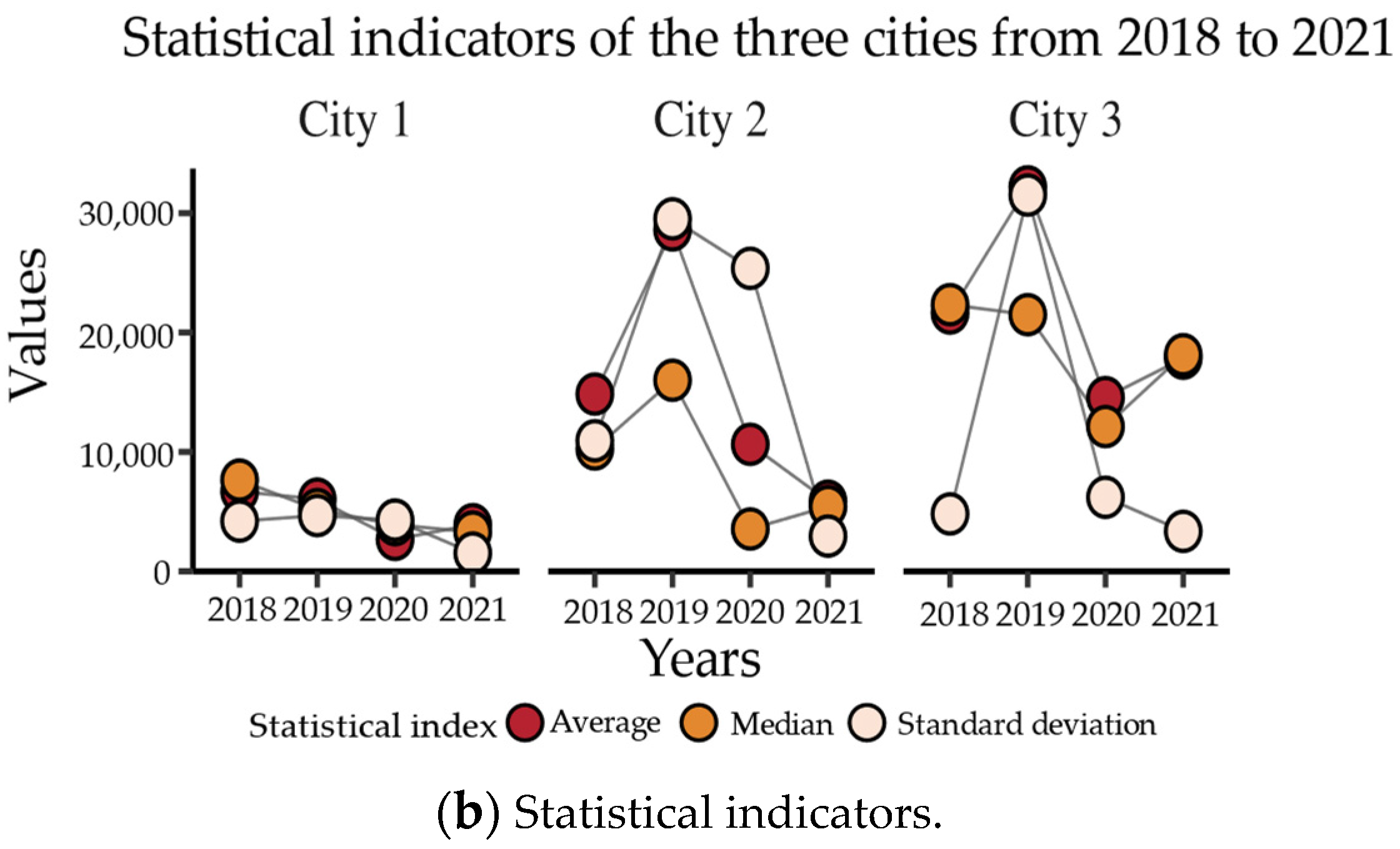
Figure 6.
(a) The number of infectious disease cases in three cities from January 2018 to August 2022; (b) statistical indicators of the three cities from 2018 to 2021.
As shown in Figure 6b, various indicators in the data for the three cities are discussed. From 2018 to 2021, the mean, median and standard deviation for City 1 were significantly lower than those for Cities 2 and 3, indicating that the epidemic scale in City 1 was smaller than in the others, on the whole. Vertically, the three indexes for City 1 are close, meaning that the distribution of the number of cases in each month is relatively average and the outbreak scale is relatively stable. The annual mean and median for Cities 2 and 3 are similar, and the difference between them and the standard deviation is large. This means that the number of cases in each month fluctuates within a similar amplitude and the scale of outbreaks is highly variable.
4.2. Demand Forecasting
After the analysis of infectious disease data in these three cities, the gray prediction method is used to predict the number of cases in the three cities from August 2021 to August 2022. The model and prediction results are evaluated. The results are reached in two ways. (1) In order to compare the results, gray prediction, SVM [29], the random forest model [30] and LSTM [31] are used to predict the data. The three criteria of the mean absolute error (MAE), mean absolute percentage error (MAPE), and root-mean-square percentage error (RMSPE) is set to measure the performance. (2) The gray prediction model is also evaluated via its own three test methods. The test results are shown in Table 2.
Table 2.
Comparison of the test indexes among the prediction methods.
For City 1 and City 2, the three indicators of the gray prediction are superior to the other three methods. For City 3, the root-mean-square of the gray prediction is slightly inferior to that of LSTM, but other indicators are also superior to those of other models. Because the gray prediction model relies on the analysis of the change rule in the short term to realize the prediction of the next stage, further analysis is conducted on the data for the three cities. It is found that the growth rate of the number of cases in City 3 from October 2018 to January 2019 is not only higher than the average growth rate of City 1 and City 2 but is also higher than the average growth rate of City 3 from January to September 2018. The change rule of data is broken in a short period of time, which means that the root-mean-square percentage of the gray prediction was slightly higher than that of the LSTM model. However, LSTM requires a large number of samples in the training process to improve its accuracy, while the gray prediction method only needs a small number of samples to complete the prediction. In addition, the gray prediction model outperforms LSTM in two of the three indexes. Given that the sample size is small, gray prediction has more advantages in dealing with this paper.
In addition to the above three indicators, gray prediction has three special testing methods. The results of the three testing methods are shown in Table 3. For the posterior difference test, when , the method is qualified; for the residual test, when and the residual test value is less than , the method is tested. For the correlation degree test, when and is greater than 0.6, it is qualified. With the results in Table 3, the values of the three indicators all meet the standards, proving that the model is suitable for this topic. The predicted results given by the gray prediction model of the number of cases in the three cities from August 2021 to August 2022 are shown in Figure 7.
Table 3.
The results of the three test criteria for gray prediction.
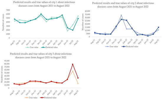
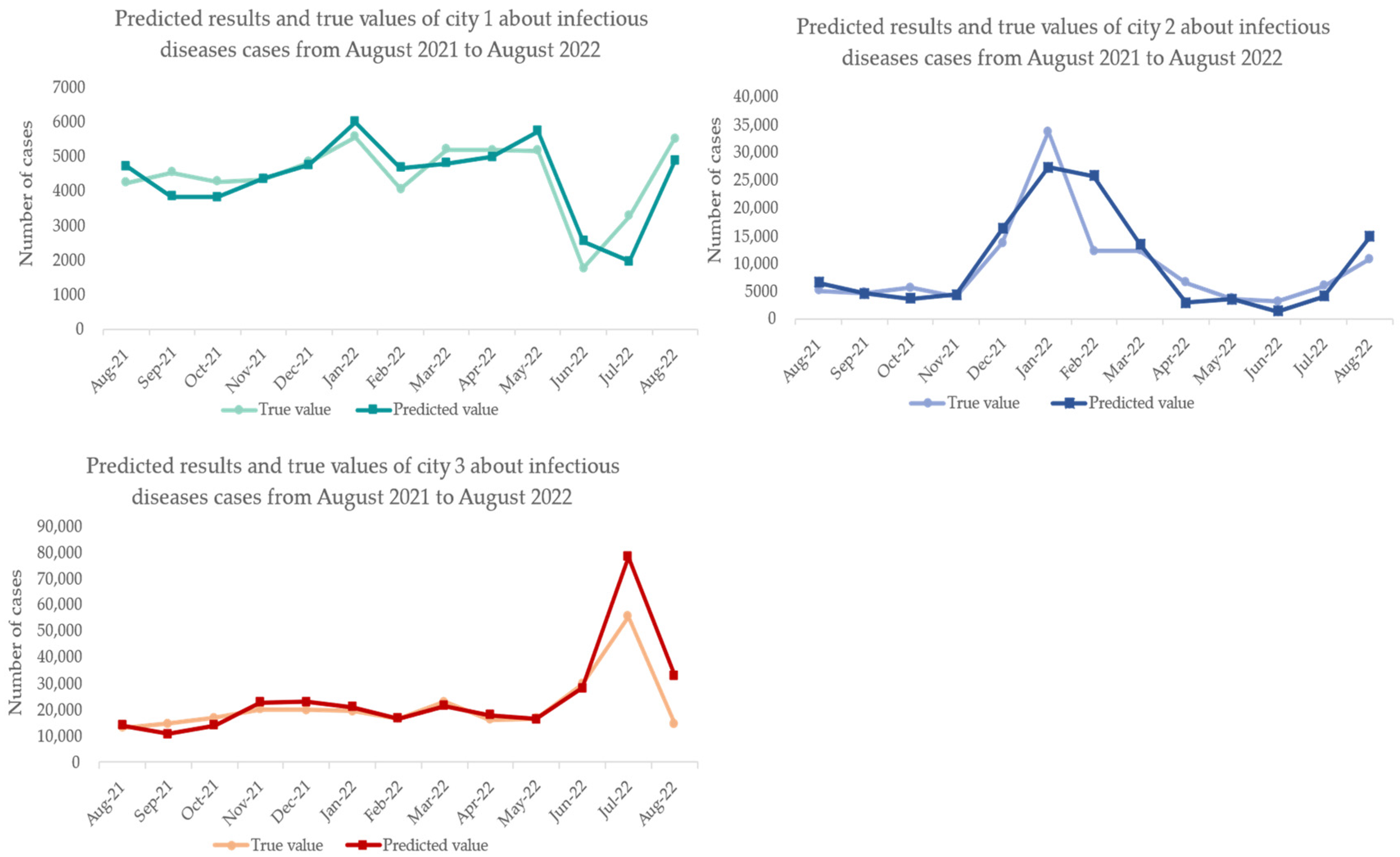
Figure 7.
The predicted results given by the gray prediction model and true values for the three cities for infectious disease cases from August 2021 to August 2022.
Compared with the above indicators, this paper uses the gray prediction model to complete the prediction job in the model. Considering that there are two parameters in the gray prediction model, the paper studied their influence on the gray prediction model by adjusting them, and the results are shown in Figure 8.
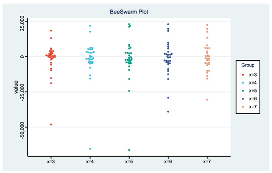
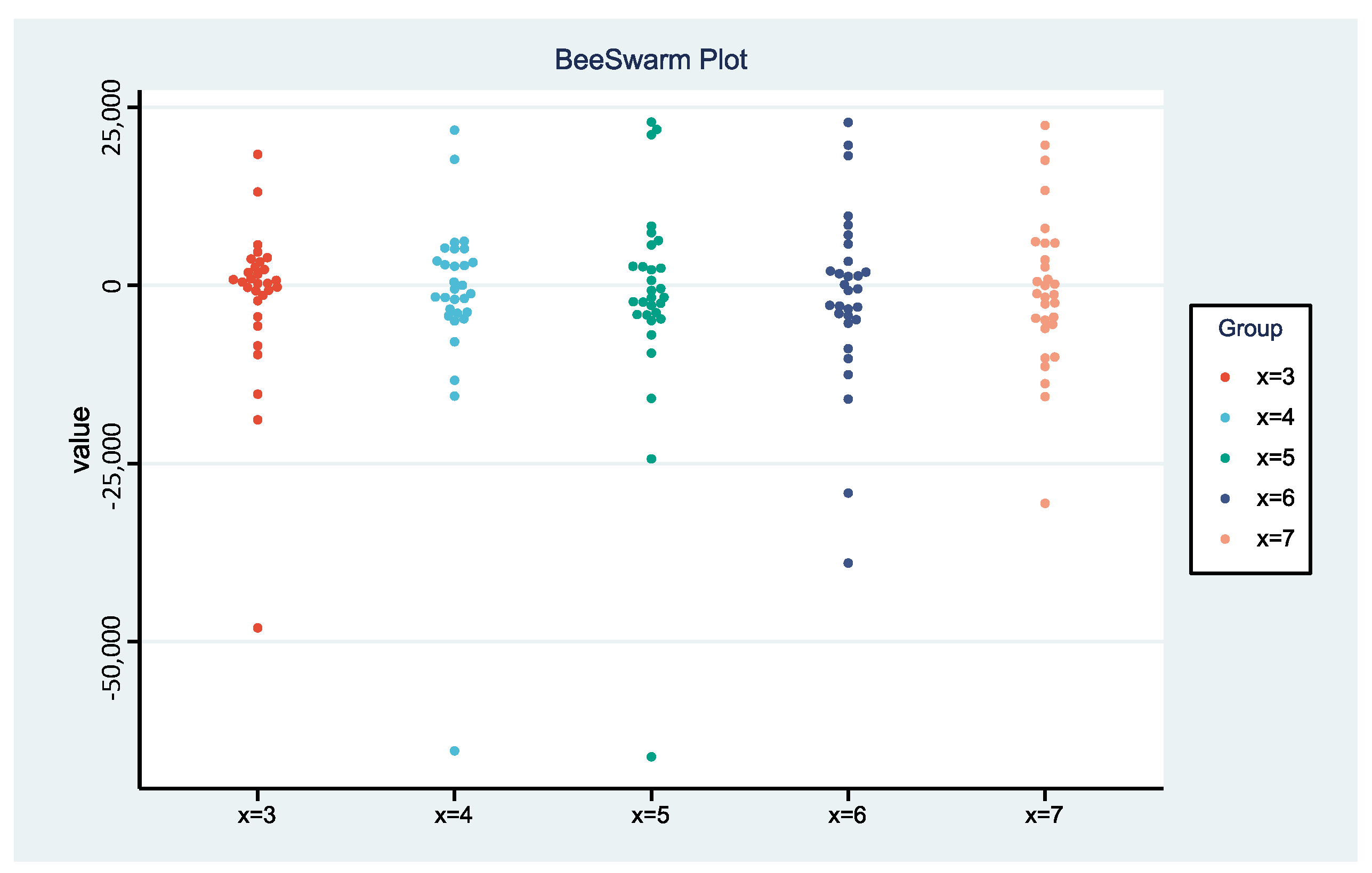
Figure 8.
The difference between the true and predicted values when .
The two parameters of the gray prediction model are the number of input variables and the number of outputs . As shown in Figure 8, we changed the value of and fix . The results generally indicate that when is fixed, the larger is, the larger the gap is between the true and predicted values. It is concluded that for every unit increase in , MAE will increase by 25.52% on average. Since the degree of dispersion is more obvious when and , the remaining three cases are chosen for further analysis. Figure 9 shows that a change in also causes a change in prediction accuracy. Increasing y will decrease the accuracy of gray prediction model. For every additional unit of , MAPE increases by 0.55 on average. By comparing the MAE and MAPE of each group and , and are finally selected.
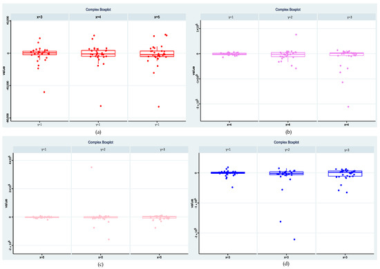
Figure 9.
(a) It shows the effect of changing on the error when ; (b–d) show the effect of changing on prediction accuracy when is fixed.
4.3. Experimental Design
As shown in Figure 7, the number of cases in City 2 increased significantly from November 2021 to December 2021 and reached 232.76% within a month. After four months, the number of infectious diseases fell back into the original range, which implies the epidemic broke out suddenly, in a short period of time. This situation is consistent with the problems discussed in this paper. Therefore, we chose City 2 as the discussed site. The period of the epidemic is set from September 2021 to April 2022, for which the unit of time denotes one month. The period from September 2021 to November 2021 is treated as the pre-stage, and the period from December 2021 to April 2022 is treated as the post-stage. Nine cities are randomly selected as the locations of suppliers, among which five are the locations of suppliers in class A and four are the locations of class B suppliers. Table 4 shows the monthly demand for materials in the epidemic area. Table 5 and Table 6 show class A and class B suppliers’ production capacity, material pricing and the distance between epidemic area and them. The gray prediction model is used to predict the number of cases from October 2021 to April 2022. According to the predicted results, the monthly demand for daily essential materials, testing materials and medical materials in epidemic areas is obtained.
Table 4.
The demand for materials per unit of time in the epidemic areas.
Table 5.
Class A suppliers’ production capacity, material pricing and transportation distance.
Table 6.
Class B suppliers’ production capacity, material pricing and transportation distance.
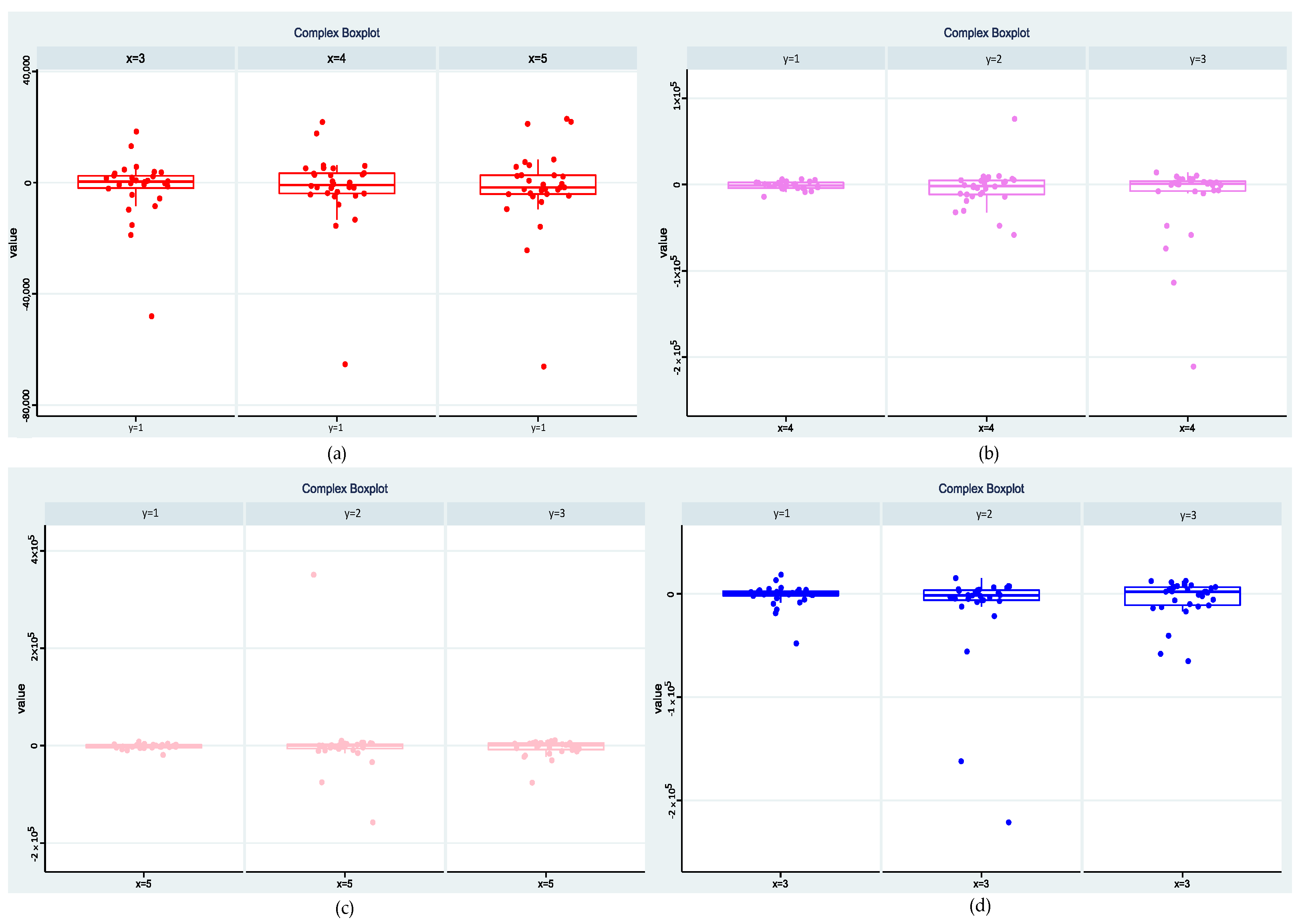
The penalty function in the objective function contains the weight coefficients. Sensitivity analysis of parameters was performed before weights were determined and the result is presented as Figure 10. ST values of are 0.36, 0.33 and 0.31, and the S1 values are the same as ST. It is concluded that generally has the same influence on the penalty value. In order to ensure that each material is of similar importance, we set and . Then, the solution for the model is compared with the solution for the random configuration model.
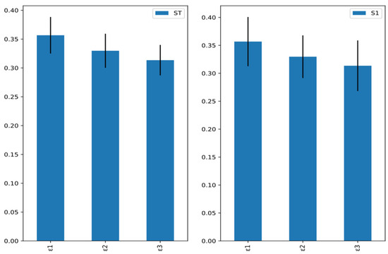
Figure 10.
Sensitivity analysis of weight parameters of penalty function.
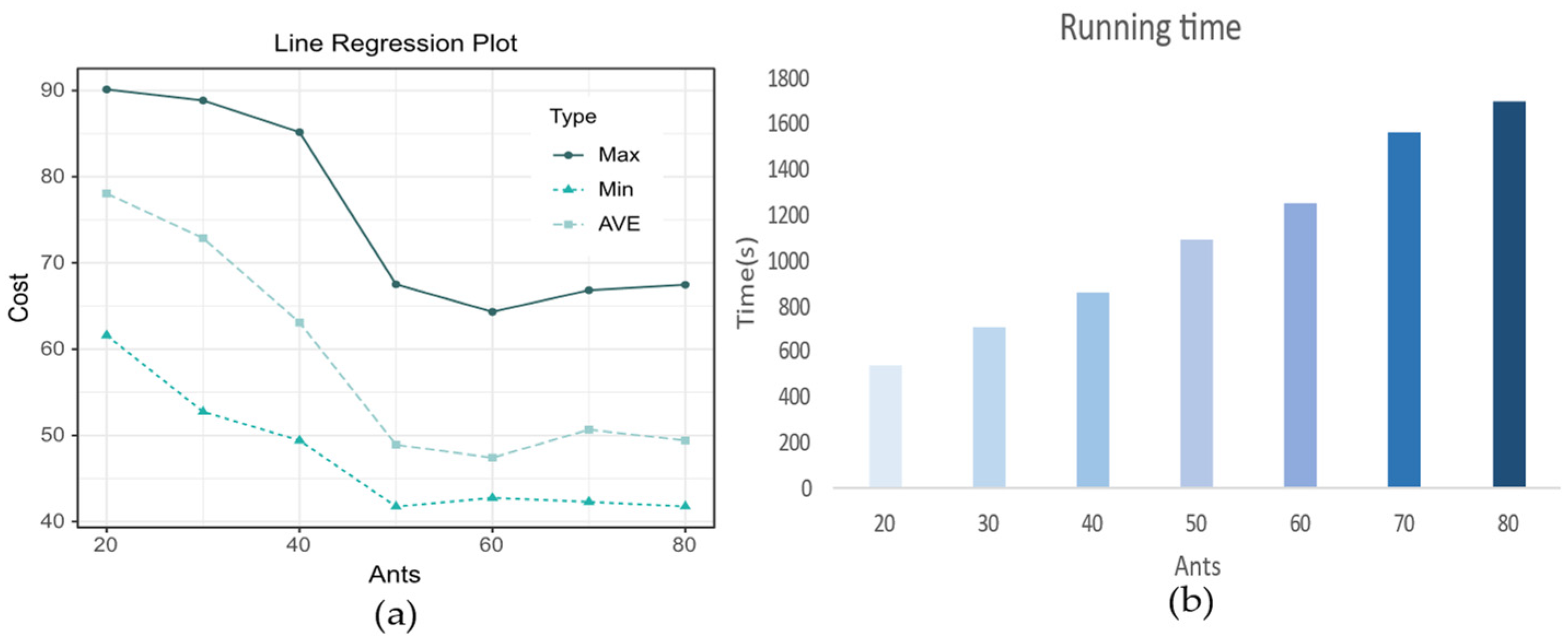
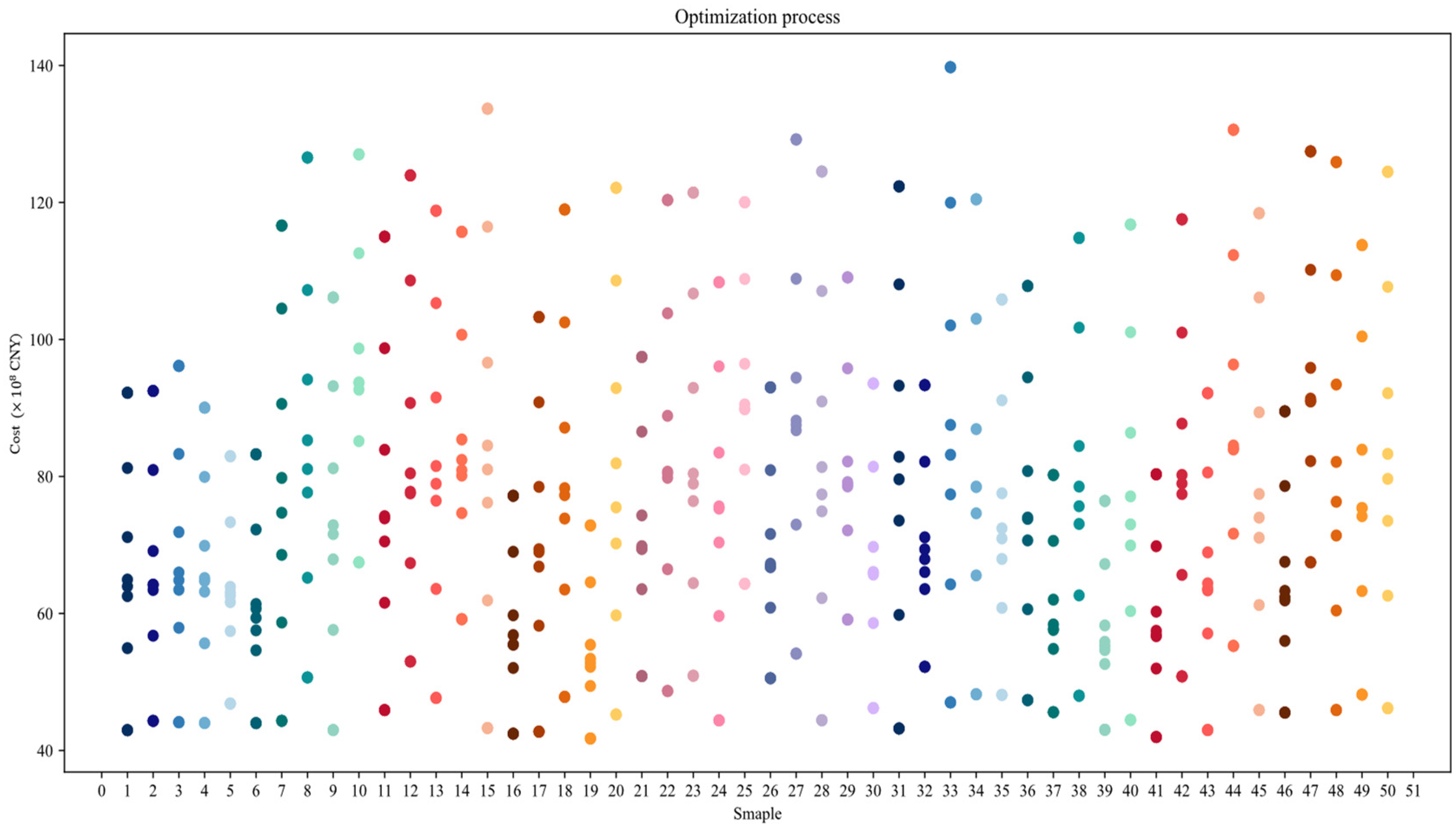
Heuristic algorithms should find a balance between intensification and diversification [32]. Therefore, extensive parameter tuning and sensitivity analysis are needed for algorithmic design. In ACO, the number of ants affect the performance of the algorithm to some extent. This paper adjusts the number of ants to compare the optimization performance and optimization time of the algorithm. Figure 11 shows the results of the comparison. Generally, as the ant population increases, the cost of the emergency plan decreases but the algorithm takes longer. The optimization results and optimization time increase by an average of 6.8% and 21.19% for each increase of 10 ants. Finally, this paper determine that the number of ants is 50. In total, 50 groups of solutions satisfying the constraint conditions are randomly generated, and these 50 groups of feasible solutions are taken as the solutions for the stochastic resource allocation model. The costs of these 50 schemes are calculated. The resource procurement allocation scheme provided by the MS-CR-U is compared with the original random scheme. At the same time, we calculate the demand satisfaction rate of the MS-CR-U to further verify the feasibility of the solution. The results are shown in Table 7. The optimization process is shown in Figure 12. Compared with the random resource allocation model, the cost of the procurement allocation scheme provided by the MS-CR-U decrease by 55.59% on average.
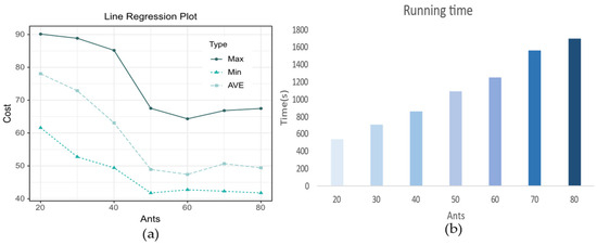
Figure 11.
The optimization performance and optimization time of the algorithm. (a) The cost of different solutions obtained by adjusting the ant population. (b) The time taken to solve the model under different ant population.
Table 7.
Comparison of the cost results of the different models.
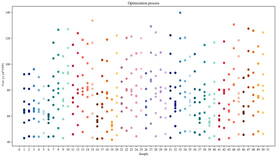
Figure 12.
The model optimization process. Different colors indicate different solutions.
is the set of decision variables for class A suppliers. When class A suppliers produce test materials, ; otherwise, . . When class B suppliers produce medical supplies, ; otherwise, . Formula (56) shows the production arrangements reached by the suppliers in class A and B and the responsible organizations. Formula (57) is the cost of the solution given by the model. Formula (58) is the penalty cost calculated using the model. The final solution given by the MS-CR-U is shown in Table 8. At this time, the required cost of the solution is CNY 4.175 billion. The penalty cost means that the solution is short of 4124 items, including 41 testing material items, 1321 medical material items, and 2762 daily essential items.
Table 8.
A and B supplier emergency materials transportation plans during the epidemic period.
To summarize, the MS-CR-U in this paper can be used to predict the number of cases in the future based on historical epidemic information and can convert the prediction results in order to obtain the demand for different materials. The requirements for various materials are taken as the input for the proposed model to generate a reasonable schedule. Thus, it is helpful in the procurement and allocation plan of emergency supplies before and after the outbreak of an epidemic. The results show that the MS-CR-U is superior to the random resource allocation model in terms of cost. Furthermore, the demand satisfaction rate of three types of emergency materials is calculated, with the guaranteed rate of living essentials being about 99.26%, the guaranteed rate of testing materials being approximately 99.27%, and the guaranteed rate of medical materials being about 99.27%. The total results prove that the scheme given by the MS-CR-U is feasible.
5. Conclusions
This paper mainly studies the method of coordinating suppliers to complete the scheduling of multiple materials in a period of time under the circumstances of uncertain demand and a dynamic epidemic situation. This paper considers the two stages, the stable period and the outbreak period, aiming to minimize the cost and meet material demand, and proposes a coordinated allocation model of multiple materials based on the gray prediction model. In view of uncertain demand, the gray prediction method is used to predict the number of confirmed cases in the following time period, and this number is utilized to estimate the possible emergency demand. Then, the Multi-catalog Schedule Considering Costs and Requirements Under Uncertainty is completed to find the final solution, which is based on the ant colony algorithm. In the proposed model, the optimization direction is represented by the adjacency matrix. The effect of selection by a single ant each time is calculated via the establishment of a utility function to adjust the probability of each direction and screen out the optimal direction. Finally, examples and related indicators demonstrate the qualifications of the model. We found that the cost of the material scheduling model is superior to other models when material demand is guaranteed. Thus, the model can provide support in decisions regarding material scheduling during an epidemic. The main consideration of this paper is the problem of demand uncertainty in emergencies. Considering the impact of emergency events on the market, the future work plan will be further discussed and studied on the influence of material price changes on decision-making based on the paper.
Author Contributions
Methodology, B.L.; software, Q.L. All authors have read and agreed to the published version of the manuscript.
Funding
This research was funded by the National Natural Science Foundation of China (72004174).
Data Availability Statement
The meteorological data come from http://www.meteomanz.com/index?l=1 (accessed on 15 September 2022). The infectious disease statistics come from https://wsjkw.sh.gov.cn/; http://wjw.beijing.gov.cn/English/; https://wsjkw.cq.gov.cn/ (accessed on 15 September 2022). No new data were created.
Conflicts of Interest
The authors declare no conflict of interest.
References
- Li, M.; Zhang, C.; Ding, M.; Lv, R. A Two-Stage Stochastic Variational Inequality Model for Storage and Dynamic Distribution of Medical Supplies in Epidemic Management. Appl. Math. Model. 2022, 102, 35–61. [Google Scholar] [CrossRef] [PubMed]
- Caunhye, A.M.; Zhang, Y.; Li, M.; Nie, X. A Location-Routing Model for Prepositioning and Distributing Emergency Supplies. Transp. Res. Part E Logist. Transp. Rev. 2016, 90, 161–176. [Google Scholar] [CrossRef]
- Fei, L.; Wang, Y. Demand Prediction of Emergency Materials Using Case-Based Reasoning Extended by the Dempster-Shafer Theory. Socio-Econ. Plan. Sci. 2022, 84, 101386. [Google Scholar] [CrossRef]
- Zhang, M.; Kong, Z. A Multi-Attribute Double Auction and Bargaining Model for Emergency Material Procurement. Int. J. Prod. Econ. 2022, 254, 108635. [Google Scholar] [CrossRef]
- Iris, C.; Cevikcan, E. A Fuzzy Linear Programming Approach for Aggregate Production Planning. In Supply Chain Management under Fuzziness; Springer: Berlin/Heidelberg, Germany, 2014; pp. 355–374. [Google Scholar]
- Zhou, J.; Reniers, G. Petri-net Based Cooperation Modeling and Time Analysis of Emergency Response in the Context of Domino Effect Prevention in Process Industries. Reliab. Eng. Syst. Saf. 2022, 223, 108505. [Google Scholar] [CrossRef]
- Zhang, X.; Lam, J.S.L.; Iris, Ç. Cold Chain Shipping Mode Choice with Environmental and Financial Perspectives. Transp. Res. Part D Transp. Environ. 2020, 87, 102537. [Google Scholar] [CrossRef]
- Zhang, Q.; Xiong, S. Routing Optimization of Emergency Grain Distribution Vehicles Using the Immune Ant Colony Optimization Algorithm. Appl. Soft Comput. 2018, 71, 917–925. [Google Scholar] [CrossRef]
- Liu, Q.; He, R.; Zhang, L. Simulation-Based Multi-Objective Optimization for Enhanced Safety of Fire Emergency Response in Metro Stations. Reliab. Eng. Syst. Saf. 2022, 228, 108820. [Google Scholar] [CrossRef]
- Liu, J.; Dong, C.; An, S. Integration and Modularization: Research on Urban Cross-Regional Emergency Cooperation Based on the Network Approach. Int. J. Disaster Risk Reduct. 2022, 82, 103375. [Google Scholar] [CrossRef]
- Feng, J.R.; Gai, W.M.; Li, J.Y. Multi-Objective Optimization of Rescue Station Selection for Emergency Logistics Management. Saf. Sci. 2019, 120, 276–282. [Google Scholar] [CrossRef]
- Wang, B.C.; Qian, Q.Y.; Gao, J.J.; Tan, Z.Y.; Zhou, Y. The Optimization of Warehouse Location and Resources Distribution for Emergency Rescue under Uncertainty. Adv. Eng. Inform. 2021, 48, 101278. [Google Scholar] [CrossRef]
- Franco, C.; Alfonso-Lizarazo, E. Optimization under Uncertainty of the Pharmaceutical Supply Chain in Hospitals. Comput. Chem. Eng. 2020, 135, 106689. [Google Scholar] [CrossRef]
- Shang, X.; Zhang, G.; Jia, B.; Almanaseer, M. The Healthcare Supply Location-Inventory-Routing Problem: A Robust Approach. Transp. Res. Part E Logist. Transp. Rev. 2022, 158, 102588. [Google Scholar] [CrossRef]
- Rebeeh, Y.; Pokharel, S.; Abdella, G.M.; Hammuda, A. A Framework Based on Location Hazard Index for Optimizing Operational Performance of Emergency Response Strategies: The Case of Petrochemical Industrial Cities. Saf. Sci. 2019, 117, 33–42. [Google Scholar] [CrossRef]
- Ferri, P.; Sáez, C.; Félix-De Castro, A.; Juan-Albarracín, J.; Blanes-Selva, V.; Sánchez-Cuesta, P.; García-Gómez, J.M. Deep Ensemble Multitask Classification of Emergency Medical Call Incidents Combining Multimodal Data Improves Emergency Medical Dispatch. Artif. Intell. Med. 2021, 117, 102088. [Google Scholar] [CrossRef] [PubMed]
- Liu, H.; Sun, Y.; Pan, N.; Li, Y.; An, Y.; Pan, D. Study on the Optimization of Urban Emergency Supplies Distribution Paths for Epidemic Outbreaks. Comput. Oper. Res. 2022, 146, 105912. [Google Scholar] [CrossRef]
- Abazari, S.R.; Aghsami, A.; Rabbani, M. Prepositioning and Distributing Relief Items in Humanitarian Logistics with Uncertain Parameters. Socio-Econ. Plan. Sci. 2021, 74, 100933. [Google Scholar] [CrossRef]
- Ceylan, Z. Short-Term Prediction of COVID-19 Spread Using Grey Rolling Model Optimized by Particle Swarm Optimization. Appl. Soft Comput. 2021, 109, 107592. [Google Scholar] [CrossRef]
- Tseng, F.M.; Yu, H.C.; Tzeng, G.H. Applied Hybrid Grey Model to Forecast Seasonal Time Series. Technol. Forecast. Soc. Change 2001, 67, 291–302. [Google Scholar] [CrossRef]
- Dorigo, M.; Di Caro, G. Ant colony optimization: A new meta-heuristic. In Proceedings of the 1999 Congress on Evolutionary Computation-CEC99 (Cat. No. 99TH8406), Washington, DC, USA, 6–9 July 1999; Volume 1472, pp. 1470–1477. [Google Scholar]
- Anzai, A.; Nishiura, H. Doubling Time of Infectious Diseases. J. Theor. Biol. 2022, 554, 111278. [Google Scholar] [CrossRef]
- Lapavitsas, C. Money and the Analysis of Capitalism: The Significance of Commodity Money. Rev. Radic. Political Econ. 2000, 32, 631–656. [Google Scholar] [CrossRef]
- Elmachtoub, A.N.; Grigas, P. Smart “Predict, Then Optimize”. Manag. Sci. 2022, 68, 9–26. [Google Scholar] [CrossRef]
- Shokouhifar, M.; Ranjbarimesan, M. Multivariate Time-Series Blood Donation/Demand Forecasting for Resilient Supply Chain Management during COVID-19 Pandemic. Clean. Logist. Supply Chain 2022, 5, 100078. [Google Scholar] [CrossRef]
- Zhu, Q.; Yang, Z.; Ma, W. A Quickly Convergent Continuous Ant Colony Optimization Algorithm with Scout Ants. Appl. Math. Comput. 2011, 218, 1805–1819. [Google Scholar] [CrossRef]
- Chew, A.W.Z.; Wang, Y.; Zhang, L. Correlating Dynamic Climate Conditions and Socioeconomic-Governmental Factors to Spatiotemporal Spread of COVID-19 via Semantic Segmentation Deep Learning Analysis. Sustain. Cities Soc. 2021, 75, 103231. [Google Scholar] [CrossRef]
- Tran, H.M.; Tsai, F.-J.; Lee, Y.-L. The Impact of Air Pollution on Respiratory Diseases in an Era of Climate Change: A Review of the Current Evidence. Sci. Total Environ. 2023, 898, 166340. [Google Scholar] [CrossRef]
- van den Burg, G.J.J.; Groenen, P.J.F. GenSVM: A generalized multiclass support vector machine. J. Mach. Learn. Res. 2016, 17, 1–42. [Google Scholar]
- Athey, S.; Tibshirani, J.; Wager, S. Generalized Random Forests. Ann. Stat. 2019, 47, 1148–1178. [Google Scholar] [CrossRef]
- Shi, X.; Chen, Z.; Wang, H. Convolutional LSTM network: A machine learning approach for precipitation nowcasting. In Proceedings of the 29th Advances in Neural Information Processing Systems, Montreal, QC, Canada, 7–12 December 2015; Volume 1, pp. 802–810. [Google Scholar]
- Iris, Ç.; Pacino, D.; Ropke, S. Improved Formulations and an Adaptive Large Neighborhood Search Heuristic for the Integrated Berth Allocation and Quay Crane Assignment Problem. Transp. Res. Part E Logist. Transp. Rev. 2017, 105, 123–147. [Google Scholar] [CrossRef]


Disclaimer/Publisher’s Note: The statements, opinions and data contained in all publications are solely those of the individual author(s) and contributor(s) and not of MDPI and/or the editor(s). MDPI and/or the editor(s) disclaim responsibility for any injury to people or property resulting from any ideas, methods, instructions or products referred to in the content. |
© 2023 by the authors. Licensee MDPI, Basel, Switzerland. This article is an open access article distributed under the terms and conditions of the Creative Commons Attribution (CC BY) license (https://creativecommons.org/licenses/by/4.0/).