
Design of a Collaborative Vehicle Formation Control Simulation Test System

1
College of Information Engineering, Shanghai Maritime University, Shanghai 201306, China
2
ZoX Technologies Co., Ltd., Shanghai 201203, China
*
Author to whom correspondence should be addressed.
Electronics 2023, 12(21), 4385; https://doi.org/10.3390/electronics12214385
Submission received: 23 September 2023
/
Revised: 13 October 2023
/
Accepted: 20 October 2023
/
Published: 24 October 2023
(This article belongs to the Special Issue Control Systems Design for Connected and Autonomous Vehicles)
Abstract
:The purpose of this research is to tackle one of the most difficult issues in the realm of self-driving cars, which is the testing of advanced self-driving application scenarios. Thus, this study proposes a simulation testing system based on hardware-in-the-loop simulation technology. This system can enable data exchange between hardware systems as well as replicate and evaluate the algorithmic operations of the equipment under laboratory conditions. The system can integrate scenario simulation software with MATLAB to evaluate algorithm performance. The vehicle formation control system is tailored for collaborative vehicle formation management scenarios and tested in the simulation test system. The findings display the functional integrity of the vehicle formation control system, the reliability of lane changing and the stability and safety of cruising. It additionally demonstrates that the simulation testing system has the ability to recreate cooperative vehicle arrangement management situations and assess their functionality and performance. In forthcoming research, comprehensive functional and performance assessments will be executed on various typical scenarios for advanced autonomous driving applications in order to authenticate the simulation test system’s applicability.
1. Introduction
Internet of Vehicles technology aims to deliver globally standardized communication tools [1] for efficiently transferring data between all participants in the transportation sector [2]. Vehicles are fitted with advanced onboard sensors, controllers, and actuators and integrate modern communication and networking technologies to achieve the exchange and sharing of intelligent information between vehicles and people, vehicles, roads, and the cloud [3]. The ongoing advancement of connected vehicle technology contributes to greater road safety and comfort, improved utilization of roads, easing of traffic congestion, provision of emergency rescue information, enhancement of the driving experience, and progress towards fully automated transport [4]. To guarantee the safe, secure and efficient functioning of smart connected vehicles in a variety of traffic and usage scenarios, extensive testing and validation, as well as a complex evolutionary process, are necessary. The testing and evaluation of functions has increasingly become the focus of research on intelligent connected vehicles both domestically and overseas [5]. However, research and development staff need to deploy vehicle-to-connection infrastructure and terminal equipment on a large scale when testing in the actual road environment, and in order to ensure the safe and reliable operation of intelligent connected vehicles in various road traffic situations, a large number of tests and validations need to be carried out in different road environments, such as urban, high-speed, and rural environments [6], and the overly large number of test scenarios and the lengthy testing time will consume a huge amount of manpower and material resources. As an important part of the development of Internet of Vehicles technology, vehicle networking in-the-loop simulation test technology can effectively reduce the test cost and improve the test efficiency, which is of great significance for the evaluation of the communication performance of V2X communication equipment, application algorithm validation and testing of Internet of Vehicles technology [7,8].
Intelligent connected vehicles in-the-loop simulation testing comprises of software simulation that combines traffic simulation software with network simulators [9] and hardware in-the-loop simulation that combines software simulation with hardware under test [10]. R. Riebl [11] utilized software simulation tools to simulate the environment in which intelligent connected vehicle devices communicate. They also examined different driver behaviors and traffic objects to evaluate parameters such as communication channel loads under various traffic conditions. However, this approach has limitations when testing proprietary intelligent transport system (ITS) devices. C. B. Math et al. [12] carried out software simulations to test diverse traffic densities and application requirements for typical road situations, which are inadequate for evaluation in other rural and urban settings. J. Wang et al. [13] created a hardware-in-the-loop simulation framework that supports real V2X in-vehicle and roadside devices. This was achieved by combining software-generated simulation scenarios and data into authentic V2X in-vehicle or roadside devices, allowing for comprehensive V2X application testing. However, the framework has intricate interfaces and doesn’t include a result analysis module. J.W. Bai [14] researched and created a testing methodology and module for V2X internet of vehicles hardware-in-the-loop simulation for the T/CSAE53-2017 application layer standard. This is utilized to execute algorithmic simulation tests for 17 application scenarios according to the national standard. P. Lei [15] developed a test methodology utilizing channel simulation for assessing the communication performance of the hardware and the performance of the autopilot algorithm.
Software simulation testing [16] is a flexible and safe way to test, which is not affected by the site, and significantly reduces the costs and time spent on testing. However, the software-simulated environment differs somewhat from the real site and has greater limitations. Hardware-in-the-loop simulation testing is a low-cost option that makes it easier to reproduce test scenarios. Algorithmic function testing is reliable and efficient when this method is used [17]. However, the majority of present hardware-in-the-loop simulation test platforms concentrate on evaluating application scenarios such as road safety, traffic efficiency, and information services. Nonetheless, there are no mature testing platforms available yet for the application scenarios put forward in the T/CSAE159-2020 application layer standard for the field of advanced intelligent driving, for instance, collaborative vehicle formation management scenarios.
To address the above issues, this paper designs a simulation test system based on hardware-in-the-loop simulation technology, aiming to test the functionality and performance of collaborative vehicle formation management scenarios. In summary, the objectives of this study can be concluded as:
- How to design a cost-effective and easily implementable testing system that can achieve functional reproduction and performance testing of advanced autonomous driving scenarios;
- How to design a sensible test scheme for collaborative vehicle formation management scenarios, including determining functional requirements and performance evaluation indexes.
The contributions of this paper can be summarized as follows:
- A vehicle formation control system is designed. Designing a control system for vehicle formations, the system comprises an auxiliary subsystem for safe lane changes and a cooperative adaptive cruise control subsystem, ensuring stable cruising of the vehicles;
- A simulation testing system, utilizing hardware-in-the-loop simulation techniques, is created to perform efficient and dependable tests on collaborative vehicle formation management scenarios;
- Functional verification and performance analysis of the vehicle formation control system are conducted within a simulation test system. The experimental results demonstrate the system’s functional completeness. Additionally, it guarantees the safety of vehicle lane changes and the safety and stability of convoy cruising. The simulation test system’s effectiveness is also demonstrated.
The paper is structured as follows. We present the design of the vehicle formation control system in Section 2, which covers the auxiliary lane change subsystem and the cooperative adaptive cruise control subsystem. Section 3 outlines the test system design, which is based on hardware-in-the-loop simulation techniques. In Section 4, we demonstrate the functional and performance testing of the vehicle formation control system within the simulation test system and analyze the simulation results. In Section 5, we examine the outcomes and provide evidence for the advantages of the study. The limitations of the system will also be mentioned. Finally, Section 6 concludes the paper and provides a future outlook.
2. Vehicle Formation Control System
Collaborative vehicle formation management application [18] involves the pilot car leading a number of follower cars in autonomous driving. The follower cars maintain a certain distance behind the pilot car and cruise in an orderly queue at a stable speed. Driving in convoy can result in reduced demand for drivers, ultimately lowering manpower costs. Furthermore, it can be highly effective in expanding road capacity, enhancing transport efficiency, and reducing air resistance of the trailing vehicle, leading to lower fuel consumption and a decrease in air pollution [19]. The practice can also yield significant benefits to improve vehicle economy and combat environmental pollution.
The vehicle formation system must facilitate the transition between the various states of creating a convoy, joining a convoy, cruising in formation, leaving a convoy, and disbanding a convoy. When a vehicle joins a convoy and a following vehicle departs, it may be necessary for the vehicle to switch lanes. In response, an auxiliary lane change subsystem is developed to determine the most suitable lane swap timing, chart a path for the vehicle to switch lanes, and facilitate lane-changing. The cooperative adaptive cruise control algorithm is utilized to achieve collaborative driving control between the lead and subsequent vehicles through V2X communication technology to maintain a specific gap and consistent velocity for cruising.
2.1. Assisted Lane Change Subsystem
2.1.1. Crash Prediction Using Minimum Longitudinal Safety Distance
It is assumed that the vehicle is travelling on a level road, as depicted in Figure 1 [20]. Car P is prepared to switch from the existing Lane 2 to the target Lane 1. Cars P1 and P4 are driving in front and behind Car P in the current lane, while Cars P2 and P3 are driving ahead and behind Car P in the target lane, respectively.
The collision scenarios can be grouped into three collision types based on the side car’s position relative to the P-car [21]. These types consist of the collision between the P-car and the front car in the present lane, the collision between the P-car and the front car in the goal lane, and the collision between the P-car and the rear car in the goal lane, shown in Figure 2.
The minimum longitudinal safety distance is used to measure whether a collision will occur when a vehicle changes lanes. It is determined by the relative longitudinal acceleration and velocity between the two vehicles, as well as the time period. Different time periods are chosen based on the lane to which the side car belongs. If the side car is a vehicle in the original lane, . If the side car is a vehicle in the target lane, . The adjustment time before vehicle P applies lateral acceleration is denoted as , and represents the moment when the vehicle enters the target lane. The minimum longitudinal safety distances, , for vehicle P and the side car are:
where represents the longitudinal acceleration of car P, represents the longitudinal acceleration of the side car, represents the speed of car P at the moment of preparation for changing lanes, and represents the speed of the side car at the moment of preparation for changing lanes.
After creating the intention to switch lanes, the vehicle initiates the judgement process for the lane change, as illustrated in Figure 3.
2.1.2. Path Planning Based on Fifth-Degree Polynomials
Commonly used methods for trajectory planning consist of artificial potential field, Bessel curve method, B-spline curve method, and curve interpolation method. A nonlinear approach for minimizing the longitudinal distance of a vehicle during an emergency lane change serves as the focus of J. Zhang et al.’s transformation of the path planning problem, which is based on B-spline curves [22]. The interior point method is utilized to solve the non-linear planning issue in order to acquire the most efficient emergency lane change avoidance path for a vehicle. H. Li et al. have conducted path planning for lane changing using multi-order Bessel curves. This technique proficiently balances lane-changing efficiency and ride comfort. However, it is restricted to constant-speed lane-changing [23]. Curve interpolation plays a vital role in lane change trajectory planning research. Polynomial interpolation is preferred due to its small computational requirements, smooth curve, and continuous curvature [24].
Cubic and fifth polynomials are the two most prevalent methods for path planning utilizing curve interpolation. Cubic polynomial interpolation guarantees the continuity of the position and velocity profiles. However, the acceleration profile may not be necessarily continuous. Fifth degree polynomial interpolation is a significant improvement over third-degree polynomial interpolation when it comes to trajectory planning. This method notably resolves the issue of discontinuous acceleration in continuous trajectories [25]. The position and velocity profiles of the trajectory, created using a fifth-degree polynomial, exhibit a continuous and smooth behavior, and the acceleration profile of the motion is also continuous, which can meet the requirements of many application scenarios. As the order increases, the obtained curve will become smoother. However, increasing the order results in a significant rise in computing resources needed. Therefore, this paper utilizes the fifth-degree polynomial interpolation method for trajectory planning.
The fifth-degree polynomial is derived by minimizing the rate of change of acceleration under various constraints, including boundary condition constraints, in order to achieve the lane change trajectory [26]. Lane change path planning, using quintic polynomials, only requires acquiring the vehicle’s starting position, velocity, and acceleration—along with the vehicle’s final position—in addition to the desired velocity and acceleration when it approaches the endpoint. Subsequently, a seamless curve that circumvents any collisions can be formulated as the lane change path [27]. The lane-change trajectory planned using the five-degree polynomial has the highest driver comfort, fewest constraints, a low shock value, and a simple computational method [28]. The fifth-degree polynomial is represented as follows:
where represents the longitudinal displacement of the vehicle and represents the lateral displacement of the vehicle. The coefficients to and to need to be determined. A smooth and continuous lane change trajectory is planned for the vehicle by calculating the lateral and longitudinal displacements of the vehicle. At the start of the vehicle lane change, its sideways movement, sideways speed, and sideways acceleration are all zero. The car travels a distance of to complete the lane change and moves sideways by a distance of . Once the lane change is complete, the sideways speed and acceleration both return to zero. Therefore, the constraints that need to be satisfied by the planning path are:
where represents the initial time of the lane change, ; represents the final time of the lane change; denotes the longitudinal velocity of the vehicle at the start of the lane change; represents the longitudinal speed of the vehicle upon completion of the lane change; denotes the longitudinal acceleration of the vehicle at the start of the lane change. The assigned coefficients are obtained by way of constraint solving.
Substituting the acquired coefficients into Equation (2) produces the equation for the path of change:
The speed at the beginning of the lane change and the longitudinal acceleration of the vehicle during the lane change are determined. Determining the duration of the alteration is sufficient for establishing the lateral and longitudinal displacement curves of the vehicle during a lane change, resulting in the trajectory of vehicle from the starting point to the endpoint.
During lane changes, excessive lateral acceleration increases the risk of sideslip or rollover. Therefore, it is essential to constrain lateral acceleration to ensure the vehicle’s lateral force does not exceed the tire adhesion constraint. The maximum level of tire adhesion is:
where represents the coefficient of adhesion between the vehicle’s tires and the road surface, and represents the acceleration due to gravity. The equations that constrain the longitudinal and lateral acceleration of the vehicle can be derived as follows:
where ay denotes the lateral acceleration of the vehicle when changing lanes. The car maintains a constant longitudinal acceleration whilst changing lanes. The lateral acceleration can be obtained by taking the second order derivative of :
2.1.3. LQR Controller-Based Trajectory Tracking
The major trajectory tracking methods that are presently employed include pure tracking algorithms founded on geometric modelling, Stanley’s algorithm, PID control algorithms based on kinematics and dynamics models, sliding mode control, and model predictive control algorithms [29,30,31]. Pacheco et al. [32] described the online performance of local path tracking control laws for mobile robots, comparing the use of PID controllers and MPC. Their findings indicate that MPC provides superior control whilst maintaining computational speed, therefore offering a more optimal solution. F. Yuan et al. [33] proposed a method for adjusting the weight coefficients of the model predictive control (MPC) controller through genetic algorithms. This can enhance the stability of the MPC controller leading to improved vehicle tracking of the target trajectory with higher response speed and accuracy. M. Park et al. developed a tandem linear quadratic regulator (LQR) controller to address the problem of robotic trajectory tracking, which effectively mitigates attitude error [34]. LQR is a type of MPC that is simpler to compute than conventional MPC. The controller parameters are easy to adjust and when the time domain is infinite, the analytical solution can still be easily obtained, ensuring the system’s absolute stability. Therefore, this paper will employ an LQR controller for trajectory tracking.
Tracking control of vehicle lane-changing trajectories using LQR [35]. The aim of LQR is to determine a set of control variables such that are simultaneously small enough. The performance index function of the system is selected as:
where and are the semi-positive definite and positive definite matrices that represent the weight matrix of the controller. The size of the error is determined by . is typically a diagonal matrix, where the diagonal elements are treated as constants or variables greater than or equal to 0. This approach aims to minimize the error vector while satisfying the optimum. measures the magnitude of control consumption, which must always be greater than 0. The Lagrange multiplier method was used to process the objective function and take partial derivatives to get control input :
where is the state matrix describing the evolutionary relationship between the state variables and is the input matrix describing the effect of the control inputs on the state variables; denotes the positive definite solution attained through solving the Riccati equation. The feedback matrix is determined:
Finally, the optimal quantity of control for the LQR controller can be obtained as follows:
2.2. Cooperative Adaptive Cruise Control (CACC) Subsystem
Car following model is an indispensable microscopic model for vehicle formation control systems. Trajectory of vehicles travelling in formation, utilizing both adaptive cruise control (ACC) and cooperative adaptive cruise control (CACC) systems, were analyzed by J. Brunner et al. [36]. The results showed that while the ACC system failed to demonstrate significant enhancement compared to human drivers, the CACC system proved to be superior in augmenting traffic flow. Q. Liu et al. [37] conducted a comprehensive traffic simulation for rear-end-collision-induced congestion, evaluating three vehicle following modes: IDM (intelligent driver model), ACC (adaptive cruise control), and CACC (collaborative ACC). Compared to IDM and ACC modes, the traffic flow in CACC mode is more stable with relatively minor speed fluctuations. The CACC system can significantly enhance road capacity and vehicle stability, and still perform well even in less intricate configurations.
The collaborative adaptive cruise control [38] implements inter-vehicle wireless communication technology to provide vehicles with real-time knowledge about their surroundings, such as the location, velocity, acceleration and other motion data of the leading vehicle and nearby vehicles. The communication network architecture for this approach is displayed in Figure 4.
Assuming that the convoy is travelling in the same lane on a straight road, the lead car in the convoy is the pilot car, numbered 1, and is followed by subsequent cars. The mathematical model for the nth subsequent car is as follows, and acceleration is obtained by deriving the velocity once:
where xn, vn and represent the position, velocity, and acceleration of the nth subsequent vehicle; stands for the distance between the nth subsequent vehicle and the n − 1th subsequent vehicle in meter; and refer to the position of the nth subsequent vehicle and the n − 1th subsequent vehicle in meter; and signifies the length of the vehicle in meters.
Reasonable workshop distance control is essential for ensuring safe and efficient driving of the vehicle fleet. Vehicle queue longitudinal control strategies are typically categorized into fixed workshop distance strategies and variable workshop distance strategies [39,40]. The fixed workshop distance strategy entails a predetermined distance between vehicles, making it easy to calculate and implement. However, it fails to cater to varying traffic conditions, leading to decreased fleet efficiency when the distance is too large when driving at low speeds and an increased risk of rear-end collisions when the distance is too small at high speeds. The strategy for adjusting the spacing between vehicles is categorized as constant time headway (CTH) [41] and variable time headway (VTH) [42], depending on whether a time headway is established with a specific value or not.
The desired workshop spacing is typically determined by the fixed workshop time distance and the current vehicle speed. The workshop spacing is set to a suitable predetermined value as required and will be adjusted according to changes in the vehicle’s speed. At moment , the safe distance between the nth vehicle is:
where represents time distance between vehicles; represents the speed of the nth vehicle at time t; denotes the braking distance of the vehicle, based on maximum deceleration. Utilizing the fixed workshop time distance approach can guarantee safer and more stable fleet driving. Meanwhile, the variable workshop time distance method involves determining the workshop time distance value in accordance with the traffic environment, aligning better with human driving tendencies; however, it is associated with more complex calculations and implementation challenges. Therefore, this paper utilizes the fixed workshop time distance method to regulate the workshop distance.
For the CACC system, the longitudinal control strategy [43,44] for maneuvering the vehicle can be stated as follows:
where represents the desired acceleration of the nth following vehicle, represents the desired acceleration of the nth following vehicle, and denote the acceleration of the pilot car and the n − 1th following car, respectively. The weight coefficients and , typically set at 0.3, are also used [45].
3. Simulation Test System
The majority of present hardware-in-the-loop simulation test platforms concentrate on evaluating application scenarios such as road safety, traffic efficiency, and information services. C. Yu et al. designed a test scenario based on hardware-in-the-loop technology to test the collision avoidance function of the in-vehicle algorithms under laboratory conditions [46]. F. Storani et al. designed a simulation test system based on hardware-in-the-loop technology for testing MPC-based traffic light control strategies [47]. D. Naithani et al. proposed an automotive hardware-in-the-loop test system to test the performance of electric vehicle control algorithms under different scenarios [48]. Classic application scenarios in the field of advanced autonomous driving, including scenarios for collaborative vehicle formation management, are proposed in the T/CSAE159-2020 application layer standard. This study presents a simulation test system that aims to reproduce the collaborative vehicle formation management scenario and assess the functionality and performance of the vehicle formation control system.
The simulation testing system comprises a software and hardware system that simulates real-life traffic scenarios for the device under test. It enables data interaction between hardware systems and conducts reproduction and testing of the algorithmic functions of the device under laboratory conditions.
The VTD (virtual test drive) simulation tool, developed by VIRES of Germany, was selected as the traffic scene visual simulation software for the simulation test system. This was used to simulate the classic road environment of vehicle formation management scenarios. It provides functions for road and traffic scene modelling, simple-yet-realistic sensor simulation, and high-precision real-time screen rendering. Firstly, a stationary scene will be established. A straight multi-lane carriageway will be selected to serve as the road setting for the scenario, offering the appropriate conditions for potential lane-changing actions of vehicles. After the road data is configured, a stationary scene file will be produced. Subsequently, the dynamic scene will be arranged based on the static scene file. Add cars as a traffic participant and provide details such as speed, acceleration, latitude, longitude, and other relevant information. Plan the proposed driving route for the car accordingly and then finalize the dynamic scene setup to build the simulation scene as illustrated in Figure 5.
The vehicle formation control system is implemented using MATLAB/Simulink to provide accurate suggestions and strategies for the maneuver of changing lanes, so that the fleet can cruise safely and orderly at a stable speed. The scenario simulation software co-simulated with Simulink can actualize the functional replication of collaborative vehicle formation management scenarios.
The ZVG-9100 instrument is chosen as the primary module for the simulation test hardware system. It features a GNSS simulator interface and a V2X simulator interface, with a TX/RX frequency range of 1.2 GHz–6 GHz, two GNSS transmitter antennas, an LTE-V2X receiver antenna, and a LTE-V2X transmitter antenna. The instrument panel is displayed in Figure 6.
Based on ZVG-9100, it is possible to carry out C-V2X simulation transceiver analysis and GNSS simulation to realistically reproduce the environmental information in the scene to the parts to be tested, thus realizing the vehicle networking hardware-in-the-loop simulation test. Extract the information of the remote vehicle and the primary vehicle from the scenario simulation software to produce V2X signals. This will enable the primary vehicle to access the position information of other vehicles on the road, such as speed, acceleration, latitude, and longitude, through the V2V signals. Simulate the CAN signals to obtain the status information of the primary vehicle, including brakes, accelerators, and turn signals. Additionally, use the GNSS simulator to emulate GNSS signals to achieve time and carrier synchronization between the V2X device and the DUT. The instrument and test device communicate with each other via air–port communication.
The design of the simulation test system is illustrated in Figure 7. The scenario library, data modules, CAN bus, GNSS simulator, and V2X simulator are all overseen by the automated test management software. Test cases are constructed using simulation software, and the interface sends simulation data to the data routing system. The data routing system manages both the tested object data and the background data. The subject data are segmented into two categories, namely the state data and the trajectory data of the primary vehicle. The state data related to the primary vehicle originates from the CAN bus, while the trajectory data of the primary vehicle is transmitted to the GNSS simulator via the GNSS interface. After the baseband signal modulation is completed to generate the RF signal, the data of the target object are transmitted to the device under test, and the background data is transmitted to the device under test via the V2X simulator. Functionally test the algorithm in the simulation scenario built by VTD and send the simulation data to MATLAB to verify and analyze the algorithm’s performance.
4. Experiments and Results
4.1. Functional Integrity Analysis of Vehicle Formation Systems
The vehicle formation control system must achieve state switching for fleet creation, joining, cruising, leaving and disbanding in order to manage processes and communicate data. A simulation scenario was created to confirm its ability to complete these state transitions. The scene simulation experiment is set up with the initial condition that the vehicle is driving on a straight road with multiple lanes, each having a width of 3.5 m. Vehicles A, B, C, and D are all 4.646 m long and equipped with wireless communication. They were driving at a constant speed on the highway at 55 km/h, 53 km/h, 53 km/h, and 50 km/h respectively.
Free Vehicle A broadcasts the command “Create convoy”, and after the successful creation, it changes its role from free vehicle to pilot vehicle and broadcasts the information table of the pilot vehicle to the outside, as shown in Figure 8a.
Free Vehicle B wants to join the convoy after receiving the convoy information from pilot vehicle A. It sets the request status to request to join the convoy, sets the convoy ID to the convoy ID of pilot Vehicle A, and broadcasts the information of requesting to join the convoy. When pilot Vehicle A accepts free Vehicle B as a member, Vehicle B sets its driving status to “Join fleet”, broadcasts the status message, and drives to the tail end of the fleet, as shown in Figure 8b,c. After Vehicle B joins the fleet, its attributes and roles are changed to the following vehicle, and it also sets its drive status to Following and broadcasts the status message. Free Vehicles C and D also follow this process to join the convoy.
After the vehicles have formed a formation, the lead car will guide them into a cruising state. The lead car will then provide the followers with the basic information sheet for both the lead car and the formation, while the following car will release the basic information sheet for itself to the public. Vehicles B, C, and D have joined the convoy and rapidly adjusted their speed to 55 km/h while optimizing the inter-vehicle spacing. Pilot Car A leads the convoy in an orderly manner, as illustrated in Figure 8d.
Car B initiates a request to depart from the convoy and receives confirmation from Pilot Car A. The travelling status is then set to “Leave the convoy” and broadcasted. Car B proceeds to change lanes and exit the convoy, as illustrated in Figure 8e. Until it has completely left the convoy, it is designated as a “Free car”.
If Pilot Car A wishes to disband the convoy, it sends a request to dismiss convoy, sets the formation status of the pilot car information sheet to request to dismiss convoy, adds all members of the convoy to the departing convoy list, and sends the pilot car information sheet. Followers C and D set their status to “Leaving convoy” and leave the convoy in turn, set their role to free vehicle and stop broadcasting convoy information when they are far away from the convoy. All followers leave the convoy, then the convoy is successfully disbanded as shown in Figure 8f. Pilot Car A’s role becomes free car, and it stops sending Pilot Car A’s information sheet.
The system for forming vehicle fleets can effectively switch between states, including fleet creation, joining, formation cruising, leaving, and disbanding, in accordance with the collaborative management of vehicle formation scenarios as defined in the national standards. This verifies the functional completeness of the vehicle formation control system.
4.2. Vehicle Lane Change Safety Analysis
The process of joining or leaving a vehicle convoy may require changing lanes. To ensure safe lane changes for vehicles, the auxiliary lane change subsystem must be effective and accurate. The working condition scenario simulation can be seen in Figure 1, and Table 1 illustrates the state parameters of each vehicle.
The collision prediction module calculates the minimum safe distance in the longitudinal direction using real-time V2X information, including the speed, acceleration, and position of the adjacent vehicle. At time = 0 s, the P-car initiates a lane change. At this moment, the longitudinal distance between the P-car and the P1-car is 7.78 m, the longitudinal distance between the P-car and the P2-car is 16.87 m, and the longitudinal distance between the P-car and the P3-car is 13.13 m. The collision prediction module calculates the minimum safe separation distances that should be maintained longitudinally between vehicle P and other vehicles—P1, P2, and P3. The specific values are = 18.2 m, = 22.6 m, = 5 m for P1-car, P2-car, and P3-car, respectively. At = 0 s, the conditions for lane change are not satisfied, and P-car receives the instruction to “Delay Lane change”. When = 2.5 s, P-car is separated from P1-car by a longitudinal distance of 18.2 m, P2-car by 30.76 m, and P3-car by 13.13 m, which satisfies lane change requirements. P-car is then instructed to “Allow to change lanes” and proceeds to make the lane change. The graph in Figure 9a illustrates the longitudinal distance change curve between the P-car and the P1, P2, and P3 cars during the lane change process. Meanwhile, Figure 9b displays the lateral position changes of the system-planned lane-changing path and the corresponding actual simulated lane-changing path during the same lane change process. Moreover, the tracking error is determined as the lateral position difference between the intended trajectory of the system and its actual simulated trajectory. Figure 9c demonstrates the error curve between the actual trajectory and the target trajectory with a maximum tracking error of 0.25 m.
The maximum tracking error is determined as the highest lateral position difference between the intended trajectory of the system and its actual simulated trajectory. In total, 1000 groups of experiments were conducted with differing speeds and workshop distances, from which the maximum tracking error value was recorded for each group. The experimental outcomes reveal that the maximum tracking error does not surpass 0.3 m. The statistical results can be seen in Figure 10.
The vehicle’s lateral position during lane changes was used as an observation index to compare lane changing trajectories planned using cubic and fifth polynomials. The experimental findings are illustrated in Figure 11. The results show that the fifth-degree polynomial generates a smoother lane-changing trajectory and process.
The experiments indicate that the supplementary subsystem for changing lanes can precisely forecast if the vehicle’s behavior of changing lanes involves a possibility of collision, map out a slick trajectory for changing lanes, and regulate the vehicle to accomplish the lane change by following the intended path, thereby ensuring its safety.
4.3. Fleet Cruise Stability Analysis
When driving on a real road, the lead vehicle accelerates and decelerates based on various working conditions. This necessitates the following vehicle to respond sensitively and promptly to the acceleration changes of the lead vehicle, guaranteeing an orderly cruise of the fleet. The pilot car travels on the road at any speed. The simulation step of the unit is 0.01 s, and the vehicle length is set at 4.646 m. There is a minimum safety clearance of 2 m, a safe following time distance of 0.6, and the control coefficients are taken as 0.45 and 0.25 [49]. Assuming a fleet size of four cars. The velocity and acceleration change curves of the subsequent vehicle controlled by the CACC model appear in Figure 12, while those of the subsequent vehicle controlled by the intelligent driver model appear in Figure 13. The results indicate that the CACC model exhibits superior following performance and faster response.
Increasing the speed of the pilot car, the velocity and acceleration change curves of the convoy according to the CACC model, along with the headway and following time distance deviation change curves, are shown in Figure 14 and Figure 15.
The findings indicate that despite an increase in the pilot car’s speed, the fleet maintains a steady and safe following distance. The subsequent car can swiftly react to changes in the leading car’s acceleration, allowing the distance between the two cars to be adjusted in time to match the speed of the fleet and ensure stable cruising. All time deviations are less than 0.04 s. The cooperative adaptive cruise control subsystem is efficacious and stable.
4.4. Fleet Cruise Safety Analysis
In fleet travel, rear-end collisions can occur when the following vehicle does not react quickly enough to the preceding vehicle’s deceleration due to high speeds or inadequate distance. Thus, it is essential to assess the safety of a vehicle’s following characteristics. In the realm of traffic safety, TTC (time to collision) is a commonly used gauge of following safety [50].
TTC refers to the point at which the front and rear vehicles maintain a uniform speed and collide with one another. If the rear vehicle’s speed is lower than the front vehicle’s, they will not collide and the TTC value is considered infinite. If the rear vehicle’s speed is equal to or greater than the front vehicle’s, the TTC value is calculated based on the relative distance and relative speed [51]:
where represents the time-to-collision value of the rear car at time ; vn(t) is the speed of car at time ; is the velocity of car at time ; indicates the position of car at time ; indicates the position of car at time ; and is the length of the bodywork of the car . Statistically, a warning for a potential vehicle collision should be given 2.5 s in advance, accounting for the driver’s reaction time and time needed to apply the brakes.
Balas et al. introduced the idea of using ITC (inverse time to collision) as a measure of collision time to assess heeling behavior. Unlike the TTC, the ITC has a smaller range of variation and better continuity, making it a more suitable safety evaluation index for the heeling behavior of a vehicle [45]. The ITC is calculated by taking the inverse of the TTC:
where, at a given moment , represents the ITC value of the rear vehicle n. If the speed of the rear vehicle is lower than the speed of the front vehicle, the ITC value is less than 0, indicating no risk of collision. Conversely, if the ITC value is greater than 0, the risk of collision is present, with greater values indicating higher risk. Fleet cruising can be considered safe and secure when the ITC value is less than 0.4.
The reciprocal change curves of fleet speed and collision time when vehicles are cruising are shown in Figure 16. No collision risk is identified when the convoy accelerates or moves at a uniform speed, indicated by a TTC value not greater than 0. In case the convoy decelerates, an ITC value greater than 0 is identified, however, none of these values exceed 0.015, indicating a small collision risk. The study demonstrates that the cooperative adaptive cruise control subsystem is capable of safely controlling the fleet while cruising, thereby indicating the reliability and safety of the subsystem.
5. Discussion
This article conducts research and analysis on current domestic and international in-the-loop simulation technology for the Internet of Vehicles, develops a vehicle formation control system for collaborative vehicle formation management scenarios, and performs functional testing and performance analysis of the vehicle formation control system in the simulation test system.
The functional completeness of the vehicle formation control system is achieved. The collaborative vehicle formation management scenario has been reproduced through the utilization of simulation software, presented in Figure 8. The system exercises control over the vehicles’ functionalities including fleet formation, joining, cruising, leaving, disbanding, and adheres to the application definition of the collaborative vehicle formation management scenario.
The algorithm for controlling the formation of vehicles is effective. As shown in Figure 9 and Figure 10, when the longitudinal distances of both the P-vehicle and the side vehicle satisfy the minimum longitudinal safety distance, the P-vehicle starts to change lanes. The observation index is the lateral position of the P-vehicle. The maximum error between the planned trajectory of the system and the lateral position of the actual simulated trajectory is no more than 0.3 m, and the safety of vehicle lane changing is guaranteed. We also compare the lane changing trajectories using cubic degree polynomial planning with those using fifth degree polynomial planning, as illustrated in Figure 11. The lane changing trajectory based on fifth degree polynomial planning is smoother and the lane changing process is accomplished more steadily. As indicated by Figure 12, Figure 13, Figure 14 and Figure 15, the CACC system can manage the following vehicles in the fleet to respond more swiftly to alterations in the lead vehicle’s acceleration. The trailing vehicle can promptly react to changes in acceleration of the leading vehicle and adjust the distance between them accordingly, with a time deviation of less than 0.04 s ensuring stable fleet cruising. As shown in Figure 16, the experimental results demonstrate that the ITC value is less than 0.015 in the process of fleet cruising. Fleet cruising can be considered safe when the ITC value is less than 0.4.
The simulation test system is both effective and justifiable. The simulation test system designed based on hardware-in-the-loop technology can simulate the real road environment under laboratory conditions. It also accurately reenacts collaborative vehicle formation management scenarios and tests the algorithms of devices under scrutiny, demonstrating the system’s practicality.
Although the proposed system performs well in experiments, there are some limitations. This paper focuses on testing the algorithm performance of the device under test in the simulation test system. Communication capabilities of the device under different scenario conditions have not been tested.
6. Conclusions
The test results have validated the reliability of the vehicle formation control system and confirmed the validity of the testing plan and simulation test system. The system for testing simulations described in this paper employs a combination of hardware-in-the-loop simulation technology, scenario simulation software, and MATLAB R2018a in order to attain functional reproduction and assess performance of scenarios for collaborative vehicle formation management. The introduction of a simulation test system for typical scenarios within the advanced intelligent driving sector ameliorates the safety and comprehensiveness of autonomous driving algorithm testing, increases testing efficiency, and further advances Internet of Vehicles technology.
The research design of this article employs vehicles that drive at slow speeds on regular highways. In future research, the potential impact of the Doppler effect on communication abilities as a result of vehicles traveling on highways will be examined. The model will be refined, and testing methods will be enhanced to further investigate this phenomenon. In the future, the algorithm’s performance will undergo examination under diverse working conditions, where multiple factors, including fluctuations in real-time weather conditions, will be accounted for to enhance the autonomous driving algorithm. Consequently, the safety and dependability of autonomous driving will be improved. Furthermore, comprehensive functional and performance assessments will be executed on various typical scenarios for advanced autonomous driving applications in order to authenticate the simulation test system’s applicability.
Author Contributions
Conceptualization, Y.Z.; methodology, Y.Z.; software, Y.Z.; validation, Y.Z.; formal analysis, Y.Z.; investigation, Z.X. and Y.Z.; resources, Z.X. and Y.Z.; data curation, Z.X., Y.Z. and F.T.; writing—original draft preparation, Y.Z.; writing—review and editing, Z.X., Y.Z., P.D. and F.T.; visualization, Y.Z.; supervision, Z.X. and P.D.; project administration, Y.Z.; funding acquisition, Z.X. All authors have read and agreed to the published version of the manuscript.
Funding
This research was funded by the National Natural Science Foundation of China, grant number No. 62271303; Pujiang Talents Plan, grant number No. 22PJD029.
Data Availability Statement
Data sharing not applicable. No new data were created or analyzed in this study. Data sharing is not applicable to this article.
Acknowledgments
The authors would like to thank all the experimental equipment and the engineering support of the HIL simulation platform from ZoX Technologies Co., Ltd., Shanghai, China.
Conflicts of Interest
The authors declare no conflict of interest.
References
- Chen, S.Z.; Hu, J.L.; Shi, Y.; Peng, Y.; Fang, J.Y.; Zhao, R.; Zhao, L. Vehicle-to-Everything (v2x) Services Supported by LTE Based Systems and 5G. IEEE Commun. Stand. Mag. 2017, 1, 70–76. [Google Scholar] [CrossRef]
- Zhong, A.; Li, Z.; Wu, D.; Tang, T.; Wang, R.Y. Stochastic Peak Age of Information Guarantee for Cooperative Sensing in Internet of Everything. IEEE Internet Things J. 2023, 10, 15186–15196. [Google Scholar] [CrossRef]
- Li, Z.; Li, F.; Tang, T.; Zhang, H.; Jin, Y. Video caching and scheduling with edge cooperation. Digit. Commun. Netw. 2022; in press. [Google Scholar]
- Abbas, F.; Fan, P.; Khan, Z. A novel low-latency V2V resource allocation scheme based on cellular V2X communications. IEEE Trans. Intell. Transp. Syst. 2018, 20, 2185–2197. [Google Scholar] [CrossRef]
- Wang, R.; Sun, Y.F.; Song, J. Evaluation method and experimental validation of road test scenarios for self-driving vehicles. Automot. Eng. 2021, 43, 620–628. [Google Scholar]
- Wang, R.M.; Deng, X.F.; Xu, Z.G. A review of research on simulation test and evaluation techniques for Internet of Vehicles. Comput. Appl. Res. 2019, 36, 1921–1926+1939. [Google Scholar]
- Yin, C.F.; Zheng, Q.; Shen, X.Q. Design of Real Network Hardware In-Loop Simulation Test Platform for Internet of Vehicles Testing. Wirel. Commun. Mob. Comput. 2023, 2023, 1895496. [Google Scholar] [CrossRef]
- Li, Z.; Zhu, N.; Wu, D.; Wang, H.G.; Wang, R.Y. Energy-Efficient Mobile Edge Computing under Delay Constraints. IEEE Trans. Green Commun. Netw. 2022, 6, 776-–786. [Google Scholar] [CrossRef]
- Maytheewat, A.; Tony, L.; Jonas, J.; Arne, N. A simulation framework for cooperative intelligent transport systems testing and evaluation. Transp. Res. Part F Traffic Psychol. Behav. 2019, 61, 268–280. [Google Scholar]
- Luisa, F.C.; David, V.; Mercè, T. Hardware-in-the-Loop Techniques for Complex Systems Analysis: Bibliometric Analysis of Available Literature. Therm. Energy Storage Effic. Util. Mater. Process Syst. 2023, 13, 8108. [Google Scholar]
- Riebl, R.; Gunther, H.; Facchi, C.; Wolf, L.C. Artery: Extending veins for VANET applications. In Proceedings of the International Conference on Models and Technologies for Intelligent Transportation Systems (MT-ITS) IEEE, Budapest, Hungary, 3–5 June 2015; pp. 2–4. [Google Scholar]
- Math, C.B.; Li, H.; Groot, S.H.; Niemegeers, I.G. V2X application-reliability analysis of data-rate and message-rate congestion control algorithms. IEEE Commun. Lett. 2017, 21, 1285–1288. [Google Scholar] [CrossRef]
- Wang, J.; Shao, Y.; Ge, Y.; Yu, R. A Survey of Vehicle to Everything (V2X) Testing. Sensors 2019, 19, 334. [Google Scholar] [CrossRef] [PubMed]
- Bai, J.W. Research and Design of Key Technologies for V2X TELEMATICS in-the-Loop Simulation Platform. Master’s Thesis, Chongqing University of Posts and Telecommunications, Chongqing, China, 2020. [Google Scholar] [CrossRef]
- Lei, P. Research on in-the-Loop Test Method of Internet of Vehicles Communication System Based on Channel Simulation. Master’s Thesis, Jilin University, Jilin, China, 2021. [Google Scholar]
- Qian, Z.T.; Xu, X.Y.; Chen, P.P. Research on software-in-the-loop simulation technology based on MATLAB/Simulink. Power Electron. 2016, 50, 5–7. [Google Scholar]
- Pavlović, T.; Župan, I.; Šunde, V.; Ban, Ž. HIL Simulation of a Tram Regenerative Braking System. Electronics 2021, 10, 1379. [Google Scholar] [CrossRef]
- Ye, X.; Lai, F.; Huo, Z. Energy Management Strategy Design and Simulation Validation of Hybrid Electric Vehicle Driving in an Intelligent Fleet. Electronics 2019, 8, 1516. [Google Scholar] [CrossRef]
- Yang, J.; Peng, W.; Sun, C. A Learning Control Method of Automated Vehicle Platoon at Straight Path with DDPG-Based PID. Electronics 2021, 10, 2580. [Google Scholar] [CrossRef]
- He, Y.M.; Feng, J.; Wei, K.; Cao, J.; Chen, S.S.; Wan, Y.N. Modeling and simulation of lane-changing and collision avoiding autonomous vehicles on superhighways. Phys. A Stat. Mech. Its Appl. 2023, 609, 128328. [Google Scholar] [CrossRef]
- Li, Y.; Zhang, R.; Li, J.; He, G. A trajectory planning based on safe distance model considering driving style. In Proceedings of the International Conference on Transportation Information and Safety (ICTIS), Xi’an, China, 4–6 August 2023; pp. 2136–2142. [Google Scholar] [CrossRef]
- Zhang, J.X.; Yang, X.; Shi, Z.T.; Zhao, J.; Zhu, B. Path Planning and Tracking Control for Emergency Lane Change and Obstacle Avoidance of Vehicles. J. South China Univ. Technol. Nat. Sci. Ed. 2020, 48, 86–93. [Google Scholar]
- Li, H.L.; Luo, Y.T.; Wu, J. Collision-Free Path Planning for Intelligent Vehicles Based on Bézier Curve. IEEE Access 2019, 7, 123334–123340. [Google Scholar] [CrossRef]
- Li, W.L.; Qiu, F.K.; Liao, D.M.; Ren, Y.P.; Yi, F. Highway lane change tracking control model based on deep reinforcement learning. J. Automot. Saf. Energy 2022, 13, 750–759. [Google Scholar]
- Huang, Y.; Zhao, M.; Zhang, J. The Position Control Method of two Joint Manipulator Based on Sliding Mode and Trajectory Setting Algorithm of Quintic Polynomial Interpolation. In Proceedings of the IEEE International Conference on Networking, Sensing and Control (ICNSC), Xiamen, China, 3–5 December 2021; pp. 1–6. [Google Scholar] [CrossRef]
- Chang, Q.; Wang, H.; Wang, D.; Zhang, H.; Li, K.; Yu, B. Motion Planning for Vibration Reduction of a Railway Bridge Maintenance Robot with a Redundant Manipulator. Electronics 2021, 10, 2793. [Google Scholar] [CrossRef]
- Zhang, Z.; Zhang, L.; Deng, J.; Wang, M.; Wang, Z.; Cao, D. An Enabling Trajectory Planning Scheme for Lane Change Collision Avoidance on Highways. IEEE Trans. Intell. Veh. 2023, 8, 147–158. [Google Scholar] [CrossRef]
- Mendonca, M.; Palacios, R.H.C.; Breganon, R.; Souza, L.B.D.; Moura, L.R.C. Analysis of the Inverse Kinematics and Trajectory Planning Applied in a Classic Collaborative Industrial Robotic Manipulator. IEEE Lat. Am. Trans. 2022, 20, 363–371. [Google Scholar] [CrossRef]
- Hu, B.B.; Zhang, H.T.; Wang, J. Multiple-target surrounding and collision avoidance with second-order nonlinear multiagent systems. IEEE Trans. Ind. Electron. 2021, 68, 7454–7463. [Google Scholar] [CrossRef]
- Chen, K.; Yamaguchi, T.; Okuda, H.; Suzuki, T.; Guo, X. Realization and evaluation of an instructor-like assistance system for collision avoidance. IEEE Trans. Intell. Transp. Syst. 2021, 22, 2751–2760. [Google Scholar] [CrossRef]
- Xu, X.; Jiang, X.W.; Xie, J.; Wang, F.; Li, M.L. Research on Human Driving Characterised Trajectory Planning and Trajectory Tracking Control Based on a Test Track. Int. J. Control Autom. Syst. 2023, 21, 1258–1272. [Google Scholar] [CrossRef]
- Pacheco, L.; Luo, N.S. Testing PID and MPC performance for mobile robot local path-following. Int. J. Adv. Robot. Syst. 2015, 12, 155. [Google Scholar] [CrossRef]
- Yuan, F.X.; Zhang, H.; Chen, F.; Si, Z.Y. Intelligent vehicle trajectory tracking control based on model prediction and genetic algorithm. J. Anhui Univ. Technol. Nat. Sci. Ed. 2021, 38, 393–400. [Google Scholar]
- Park, M.; Kang, Y. Experimental verification of a drift controller for autonomous vehicle tracking: A circular trajectory using lqr method. Int. J. Control. Autom. Syst. 2020, 19, 404–416. [Google Scholar] [CrossRef]
- Xu, X.W.; Cui, J.R.; Yan, Y.B.; Ma, J.M.; Wang, Y.W. Research on autonomous lane-changing overtaking control method for intelligent vehicles. J. Wuhan Univ. Sci. Technol. 2023, 46, 225–233. [Google Scholar]
- Brunner, J.S.; Makridis, M.A.; Kouvelas, A. Comparing the Observable Response Times of ACC and CACC Systems. IEEE Trans. Intell. Transp. Syst. 2022, 23, 19299–19308. [Google Scholar] [CrossRef]
- Liu, Q.C.; Ouyang, W.; Zhao, J.Y.; Cai, Y.F.; Chen, L. Fuel Consumption Evaluation of Connected Automated Vehicles under Rear-End Collisions. Promet Traffic Transp. 2023, 35, 331–348. [Google Scholar] [CrossRef]
- Wang, Z.; Gao, Y.; Fang, C.; Liu, L.; Zeng, D.; Dong, M. State-estimation-based control strategy design for connected cruise control with delays. IEEE Syst. J. 2023, 17, 99–110. [Google Scholar] [CrossRef]
- Li, S. Research on Humanized Longitudinal Control of Automobile Queue. Master’s Thesis, Jilin University, Jilin, China, 2023. [Google Scholar]
- Yu, X.H.; Guo, G. A generalized variable time-distance strategy in fleet control. J. Autom. 2019, 45, 1335–1343. [Google Scholar] [CrossRef]
- Luu, D.; Lupu, C.; Alshareefi, H. A Comparative Study of Adaptive Cruise Control System based on Different Spacing Strategies. J. Control. Eng. Appl. Inform. 2022, 24, 3–12. [Google Scholar]
- Li, Y.F.; Lu, Q.X.; Zhu, H.; Li, H.Q.; Li, H.Q.; Hu, S.; Yu, S.Y.; Wang, Y.B. Variable Time Headway Policy Based Platoon Control for Heterogeneous Connected Vehicles with External Disturbances. IEEE Trans. Intell. Transp. Syst. 2022, 23, 21190–21200. [Google Scholar] [CrossRef]
- He, H.; Liu, D.; Lu, X.; Xu, J. ECO Driving Control for Intelligent Electric Vehicle with Real-Time Energy. Electronics 2021, 10, 2613. [Google Scholar] [CrossRef]
- Li, Z.; Deng, Y.; Sun, S. Adaptive Cruise Predictive Control Based on Variable Compass Operator Pigeon-Inspired Optimization. Electronics 2022, 11, 1377. [Google Scholar] [CrossRef]
- Ren, R.Y. Simulation Study of Cooperative Adaptive Cruise Control Fleet. Master’s Thesis, Kunming University of Science and Technology, Kunming, China, 2020. [Google Scholar] [CrossRef]
- Yu, C.H.; Chen, Y.Z.; Kuo, I.C. The benefit of Simulation Test Application on the Development of Autonomous Driving System. In Proceedings of the International Automatic Control Conference (CACS) 2020, Hsinchu, Taiwan, 4–7 November 2020; pp. 1–5. [Google Scholar] [CrossRef]
- Storani, F.; Pace, R.D.; Luca, S.D. Hardware-in-the-Loop and Traffic-in-the-Loop for Testing Cooperative Intersection Management. In Proceedings of the IEEE International Conference on Environment and Electrical Engineering and IEEE Industrial and Commercial Power Systems Europe (EEEIC/I&CPS Europe) 2023, Madrid, Spain, 6 June 2023; pp. 1–5. [Google Scholar] [CrossRef]
- Naithani, D.; Khandelwal, R.R.; Garg, N. Development of an Automobile Hardware-in-the-Loop Test System with CAN Communication. In Proceedings of the Second International Conference on Augmented Intelligence and Sustainable Systems (ICAISS), Trichy, India, 23–25 August 2023; pp. 1653–1656. [Google Scholar] [CrossRef]
- Hao, W.; Yu, H.J.; Gao, Z.B. CACC traffic management strategy under the influence of autopilot-only lanes. Chin. J. Highw. 2022, 35, 230–242. [Google Scholar] [CrossRef]
- Li, C.; Chen, H.; Xiong, Y.; Chen, Y.; Zhao, S.; Duan, J.; Li, K. Analysis of Chinese Typical Lane Change Behavior in Car–Truck Heterogeneous Traffic Flow from UAV View. Electronics 2022, 11, 1398. [Google Scholar] [CrossRef]
- Zhang, L.; Yu, Z.; Xu, X.; Yan, Y. Research on Automatic Emergency Braking System Based on Target Recognition and Fusion Control Strategy in Curved Road. Electronics 2023, 12, 3490. [Google Scholar] [CrossRef]
Figure 1.
Lane changing scenarios.

Figure 2.
Example collision scenarios. (a) Collision with the vehicle in the current lane; (b) collision with a vehicle ahead of the target lane; (c) collision with a vehicle behind the target lane.
Figure 2.
Example collision scenarios. (a) Collision with the vehicle in the current lane; (b) collision with a vehicle ahead of the target lane; (c) collision with a vehicle behind the target lane.

Figure 3.
Vehicle formation control system lane change judgement process.

Figure 4.
Vehicle communication architecture based on wireless technology.

Figure 5.
VTD simulation scenario construction.

Figure 6.
ZVG-9100 panel.

Figure 7.
Simulation test system architecture.

Figure 8.
Functional simulation of vehicle formation system. (a) Creates a convoy; (b) joining the convoy; (c) Vehicle B joins the convoy successfully; (d) convoy cruise; (e) Follow Car B is leaving the convoy. (f) The convoy is successfully disbanded.
Figure 8.
Functional simulation of vehicle formation system. (a) Creates a convoy; (b) joining the convoy; (c) Vehicle B joins the convoy successfully; (d) convoy cruise; (e) Follow Car B is leaving the convoy. (f) The convoy is successfully disbanded.
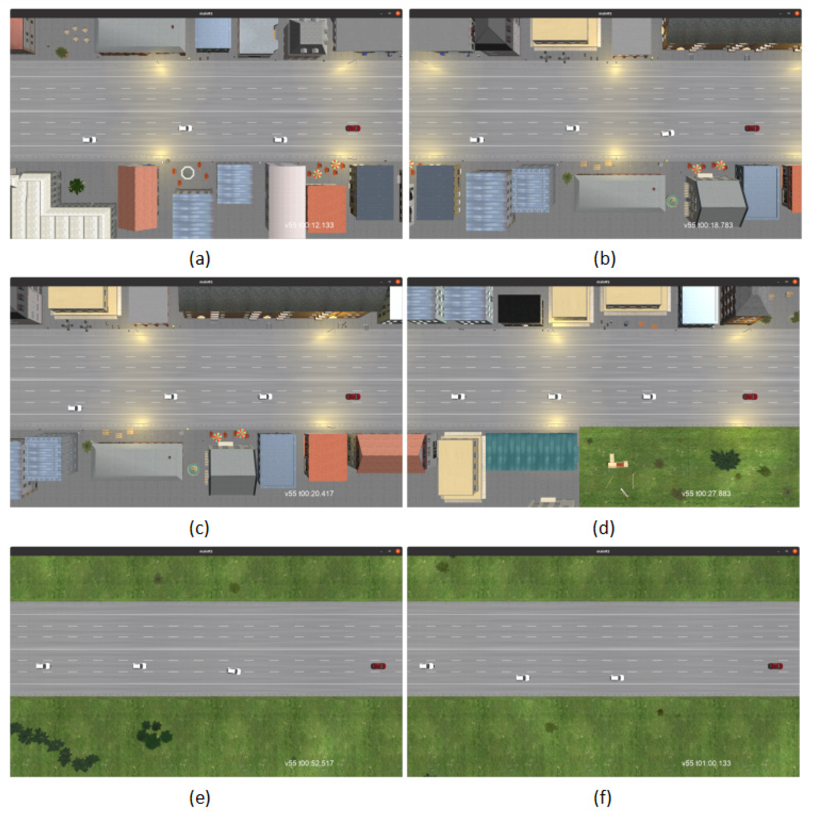
Figure 9.
Simulation results of workplace lane changing. (a) Longitudinal distance between car P and cars P1, P2, and P3; (b) compare the target trajectory with the actual trajectory lateral position.; (c) error between target trajectory and actual trajectory.
Figure 9.
Simulation results of workplace lane changing. (a) Longitudinal distance between car P and cars P1, P2, and P3; (b) compare the target trajectory with the actual trajectory lateral position.; (c) error between target trajectory and actual trajectory.

Figure 10.
Maximum tracking error statistics of 1000 sets of experiments.

Figure 11.
Path planning based on cubic polynomials, fifth polynomials.

Figure 12.
Follow the velocity and acceleration change curve of the vehicle (CACC).

Figure 13.
Follow the velocity and acceleration change curve of the vehicle (IDM).

Figure 14.
Vehicle speed and acceleration profiles.sange.

Figure 15.
Variation curves of headway and following time deviation.

Figure 16.
Vehicle speed and ITC value change curves.


Table 1.
Simulation state parameters.
| Vehicle ID | Initial Coordinates (m) | Initial Velocity (km/h) | Accelerations (m/s2) |
|---|---|---|---|
| P | (1.75, 0.00) | 60 | 0.3 |
| P1 | (1.75, 7.78) | 75 | 0 |
| P2 | (5.25, 16.87) | 80 | 0 |
| P3 | (5.25, −13.13) | 60 | 0 |
| P4 | (1.75, −18.06) | 50 | 0 |
Disclaimer/Publisher’s Note: The statements, opinions and data contained in all publications are solely those of the individual author(s) and contributor(s) and not of MDPI and/or the editor(s). MDPI and/or the editor(s) disclaim responsibility for any injury to people or property resulting from any ideas, methods, instructions or products referred to in the content. |
© 2023 by the authors. Licensee MDPI, Basel, Switzerland. This article is an open access article distributed under the terms and conditions of the Creative Commons Attribution (CC BY) license (https://creativecommons.org/licenses/by/4.0/).
Share and Cite
MDPI and ACS Style
Xu, Z.; Zhang, Y.; Ding, P.; Tu, F. Design of a Collaborative Vehicle Formation Control Simulation Test System. Electronics 2023, 12, 4385. https://doi.org/10.3390/electronics12214385
AMA Style
Xu Z, Zhang Y, Ding P, Tu F. Design of a Collaborative Vehicle Formation Control Simulation Test System. Electronics. 2023; 12(21):4385. https://doi.org/10.3390/electronics12214385
Chicago/Turabian StyleXu, Zhijing, Yuqiong Zhang, Pengren Ding, and Fangze Tu. 2023. "Design of a Collaborative Vehicle Formation Control Simulation Test System" Electronics 12, no. 21: 4385. https://doi.org/10.3390/electronics12214385
Note that from the first issue of 2016, this journal uses article numbers instead of page numbers. See further details here.