Abstract
Reinforcement Learning (RL) has been employed to assign transmission parameters to all sub-carriers in a set frequency band for anti-jamming Orthogonal Frequency Division Multiplexing (OFDM) systems. However, prior works often overlooked the influence of wireless environment fading and convergence issues stemming from overly large parameter sets. To address these challenges, an anti-jamming scheme was proposed based on the Non-Contiguous Orthogonal Frequency Division Multiplexing (NC-OFDM) communication system integrated with reinforcement learning. First, all sub-carriers were divided into sub-bands, and a Finite State Markov Sub-bands (FSMS) model was established to describe the time-varying fading characteristics of each sub-band by combining Adaptive Modulation and Coding (AMC) technology. To mitigate instability due to the fading channel, a joint sub-band and modulation anti-jamming decision scheme was adopted, enabling the transmitter to select the optimal sub-band and transmission rate. Ultimately, this decision-making process was modeled as a Markov Decision Process (MDP), and an Upper Confidence Bound based Q-learning (UCB-Q) anti-jamming algorithm was proposed for obtaining the joint sub-band and transmission rate selection strategies. Simulation results indicate that the proposed algorithm demonstrates enhanced speed and superior average throughput. Additionally, the algorithm showcases the same commendable anti-jamming performance in scenarios with time-varying dynamic jamming.
1. Introduction
Efficient, reliable, and high-quality transmission is a crucial aim in modern and future wireless communication [1]. Wireless communication transmission faces challenges from two main aspects [2]. On the one hand, because of the multipath fading characteristic and diversity of the radio wave propagation environment, the wireless channel can be very complex and variable. On the other hand, due to the open and shared nature of wireless communication, it is highly vulnerable to different jamming signals, both natural and malicious.
To prevent multipath fading and malicious jamming, data transmission often needs to occur on undisturbed frequency bands, leading to discontinuities in the transmission frequency. NC-OFDM, a variant of OFDM, has the benefits of simple implementation, high spectrum utilization, and strong fading resistance compared with OFDM systems. In addition, it can configure sub-carriers flexibly based on the distribution of non-continuous spectra. Therefore, NC-OFDM is considered an ideal transmission technique for communication in jamming environment [3,4,5].
To combat the malicious jammer, various methods like power control [6,7], rate control [8,9], and spatial multiplexing [10,11] have been used in traditional OFDM techniques. These methods commonly use channel state information (CSI) to adjust transmission parameters for maximum link throughput. However, the primary shortcoming of these methods is their reliance on channel estimation accuracy. The effectiveness of these strategies will be reduced if the channel estimation accuracy is low. To decrease the reliance on channel estimation, previous studies use Cognitive Radio (CR) technology to create cognitive anti-jamming optimization models for OFDM transmission parameters such as sub-carriers, power, and modulation coding schemes and suggest corresponding optimization algorithms to decide the best communication strategy. For example, in [12], an enhanced particle swarm algorithm is suggested for optimizing spectrum resource allocation. In [13], a heuristic algorithm-based multi-parameter decision engine is explored and in [14] delves into cognitive anti-jamming systems that use intelligent decision-making based on the Artificial Bee Colony algorithm. The optimization algorithms mentioned above are based on mathematical models and may not perform well in real-life scenarios that deviate from the theoretical model. If the interference changes rapidly, optimization algorithms may require more computational resources and anti-jamming methods may become ineffective. Therefore, discovering an intelligent technique to prevent interference is crucial.
Machine learning algorithms have gained attention for addressing the challenges of dynamic jamming environments, leading to the emergence of intelligent anti-jamming technologies. The authors of [15,16,17] summarize the latest machine learning-based anti-jamming technologies in cognitive radio applications. The wireless channel environment is often assumed to be ideal in existing research, ignoring the ever-changing nature of wireless environments caused by multipath effects and Doppler shifts. Moreover, the majority of researches regard sub-carriers as the fundamental elements for transmission parameter distribution, elevating the computational burden of the algorithms. In order to address the time-varying nature of channel fading, the FSMS model was utilized to account for the time-dependent channel fading. Parameters were allocated to multiple sub-carriers by dividing them into sub-band units.
In this paper, the joint transmission parameter selection problem of sub-band and transmission rate in NC-OFDM communication systems is addressed, specifically in wireless environments with both channel fading and malicious jamming. The decision-making process is modeled using Markov Decision Processes (MDP) with the objective of maximizing communication throughput, and the Q-learning method is adopted to solve the MDP. One of the challenges in this study arises from the necessity for the agent to select both the transmission sub-band and rate as parameters. This results in large action and state spaces, complicating the convergence of conventional Q-learning to the optimal value. Inspired by [18], a modified Q-learning anti-jamming algorithm that combines the confidence interval in the UCB algorithm with Q-learning is proposed.
The main contributions of this paper are summarized as follows:
- Unlike prior research that employed sub-carriers as allocation units for OFDM systems, the sub-carriers are divided into sub-band units to decrease the decision space of the system. Meanwhile, the FSMS model is used to determine the time-varying properties of the transmission rates of these sub-bands under the fading environment.
- A jamming-aware transmission parameter selection scheme is proposed to enhance transmission stability in fading and jamming environments. This scheme selects the transmission sub-band and rate by sensing the wireless environment, which transforms the selection challenge into an MDP problem.
- To address the challenges presented by a vast action and state spaces, a modified Q-learning algorithm based on confidence intervals is introduced. The algorithm combines Q-learning with confidence in the UCB algorithm to balance exploration and exploitation in action selection. Since it does not require prior knowledge of interference and quickens the convergence to the optimal value, the proposed algorithm can be widely applied.
The rest of the paper is organized as follows. Section 2 introduces the system model. Section 3 presents the joint problem of multiple sub-bands and transmission rate selection, which is formulated as an MDP problem. Section 4 proposes a modified Q-Learning algorithm based on confidence intervals, which has been proved to converge to the optimal strategy. Simulation results and analysis are provided in Section 5. The conclusion is drawn in Section 6.
2. System Model
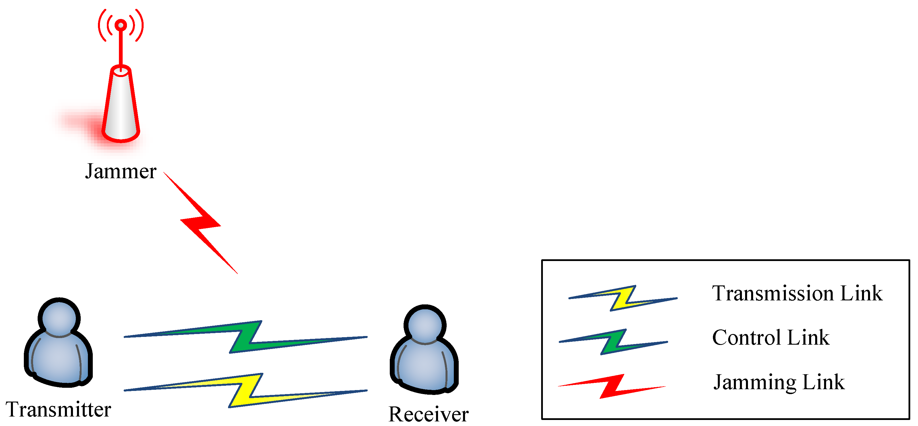
Figure 1 presents a classical wireless communication scenario where a pair of communicating users (Tx-Rx pairs) transmit data through both the transmission link and the control link, while simultaneously facing potential disruptions from an adversarial jammer. The jammer’s objective is to interfere with inter-user communication to the greatest extent possible. The communication mechanism adopted by the users employs the NC-OFDM technology, a contemporary transmission technique renowned for its spectral efficiency, especially in fluctuating environmental conditions.

Figure 1.
Wireless communication scenario.
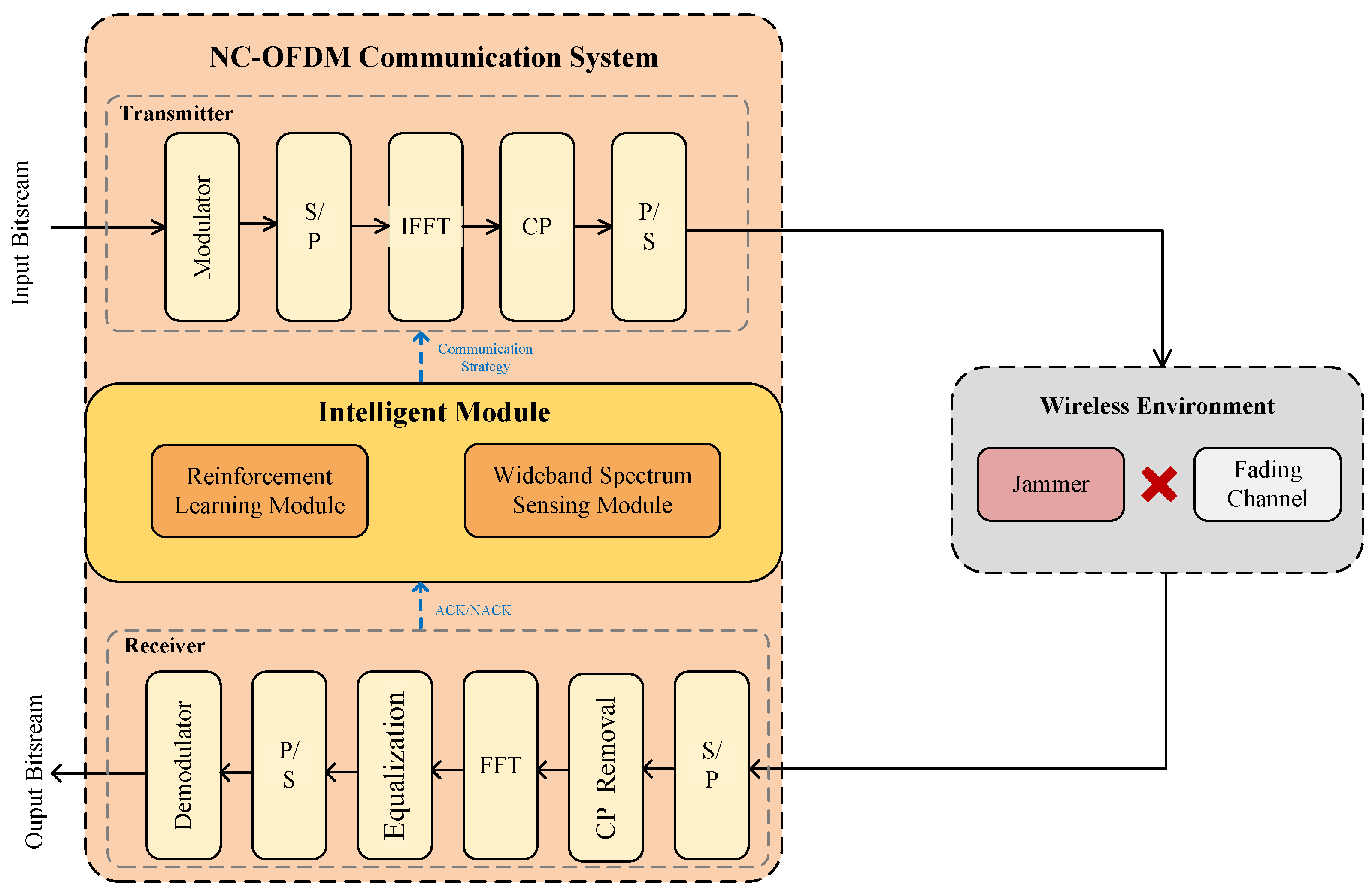
The NC-OFDM communication system comprises two main components: an intelligent module designed to adapt to real-time conditions in the wireless environment and a configurable NC-OFDM communication module. Channel fading and malicious jamming in transmission links are considered to be the primary determinants of communication quality. Specifically, channel fading limits the maximum achievable transmission rate of a link, while jammers disrupt communication by varying their frequency using methods such as linear sweep, random sweep, and random jamming. Notably, users cannot obtain the relevant parameters of the jammer. Instead, the devised communication strategy depends on the Wideband Spectrum Sensing (WBSS) capabilities of the intelligent module and the subsequent ACK/NACK feedback from the control link after strategy application. A more detailed representation of the NC-OFDM communication system model can be found in Figure 2.
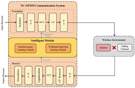
Figure 2.
Communication system model.
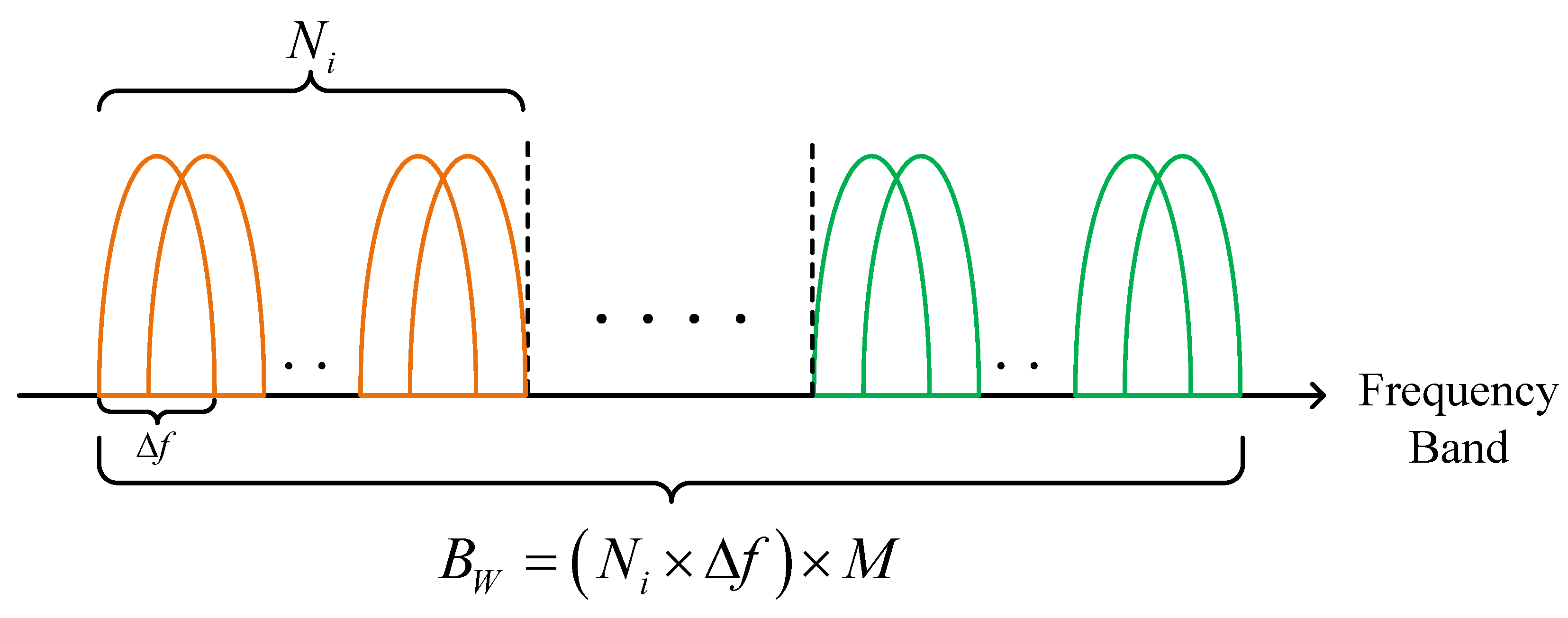
It is assumed that the point-to-point communication link between Tx and Rx comprises sub-carriers within a bandwidth of (Hz). Typically, the number of sub-carriers in an OFDM system closely matches to the IFFT points. Therefore, when faced with many sub-carriers and limited spectral resources, the entire OFDM band can be partitioned into non-overlapping contiguous sub-bands, as depicted in Figure 3. Given that the bandwidth of each sub-carrier is and that sub-bands have an equal number () of sub-carriers matched with a sub-channel, sub-carriers within a sub-band adopt identical transmission parameters for data transfer. Designating transmission parameters with sub-bands as the primary unit simplifies allocation units, thereby reducing the algorithmic complexity for sub-carrier assignment. The set of sub-bands available to the user is denoted as .
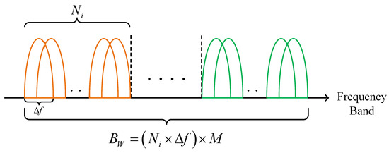
Figure 3.
Schematic diagram of the sub-banding method.
In the IEEE 802.11a standard [19,20,21], the Adaptive Modulation and Coding (AMC) approach is commonly adopted to examine the effect of channel transmission rates on communication systems. The communication system employing AMC dynamically alters its transmission rate by adaptively adjusting its modulation scheme and coding efficiency. For instance, when a low Signal-to-Noise Ratio (SNR) is detected at the receiver, it suggests suboptimal channel conditions, and transmission might be best carried out using the BPSK mode for a lower bit rate. Conversely, when a high SNR is received, this indicates favorable channel conditions, enabling transmission via the 64-QAM mode for a higher bit rate. As illustrated in [22], Table 1 lists the transmission modes associated with the AMC approach in the IEEE 802.11a standard as well as the modulation schemes, coding efficiency, bit rates, and other key communication parameters for each mode. Given a constant symbol rate, each mode in Table 1 corresponds to a specific transmission rate.

Table 1.
Convolutional coded based transmission modes and parameters for AMC communication.
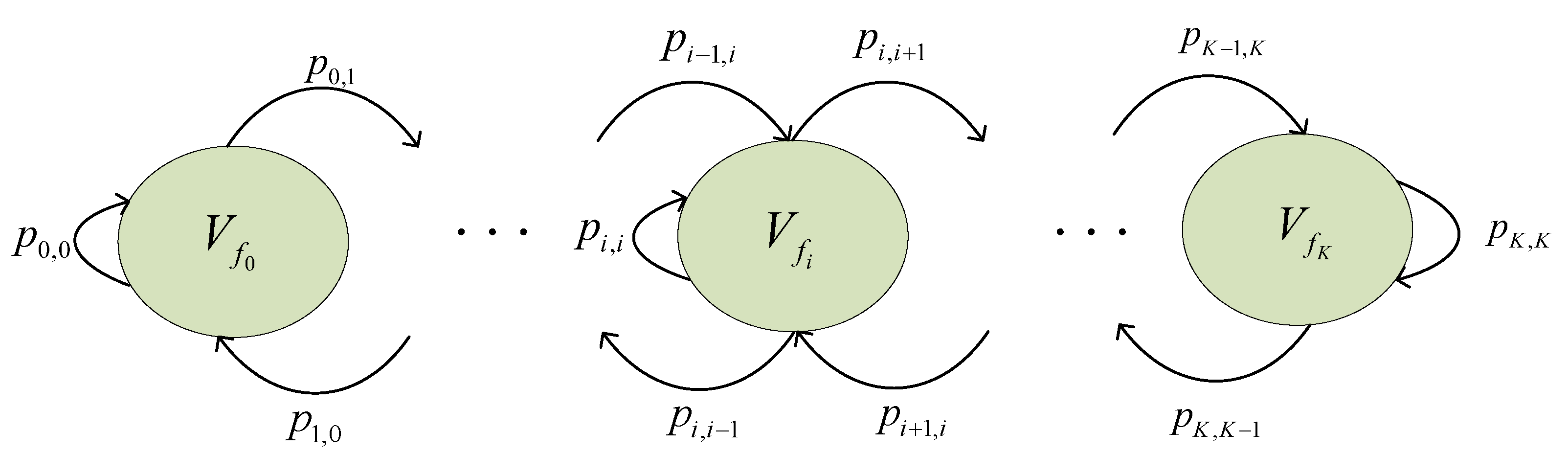
In wireless transmission links, the receiver’s SNR undergoes variations due to channel fading. Consequently, the received SNR can serve as an effective metric to evaluate channel quality. Utilizing AMC technology, the maximum transmission rate of each sub-band into K states, influenced by the received SNR’s probability density function and the target Packet Error Rate (PER). The set of the maximum transmission rate that each sub-band can support is denoted as (), where signifies the sub-band maximum transmission rate. Such a rate can be obtained through the Markov sub-band model and reflects the channel quality. Each sub-band transmission rate corresponds to a transmission mode, with the set of transmission mode levels represented as . To capture sub-band transmission rate fluctuations in fading environments, the Finite State Markov Sub-bands (FSMS) model [23,24,25] is introduced. The core concept is to correlate sub-band transmission rates with distinct Markov states. Amid state transitions, a sub-band state might either remain consistent or transition to an adjacent state. Figure 4 depicts a Markov chain that representing these sub-band transmission rate state shifts.
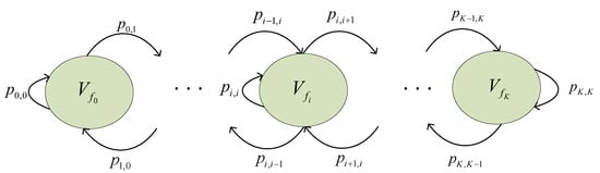
Figure 4.
Markov transition diagram for sub-band transmission rate states.
All sub-carriers within a sub-band are assumed to experience the same fading. According to [26,27], sub-band fading is frequency-flat, which indicates that the sub-band transmission rate remains constant within each transmission time slot but may vary in subsequent time slots. Different modulation modes can be employed for transmission between user pair, and adaptive decoding is implemented at receiver. The symbol rate for each modulation mode is constant within the system, and the set of transmission rates is denoted by . Figure 5 shows the relationship between the achievable communication transmission rate and the sub-band transmission rate for a sub-band transmission rate. For , when , only rate can be decoded at Rx. This paper operates on the assumption that if the transmission occurs at or above a certain rate, but the sub-band rate is below this, the transmitted data will be entirely lost.
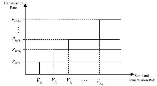
Figure 5.
Schematic diagram of realizable communication transmission rate and sub-band transmission rate.
2.1. OFDM Transmission Frame Structure
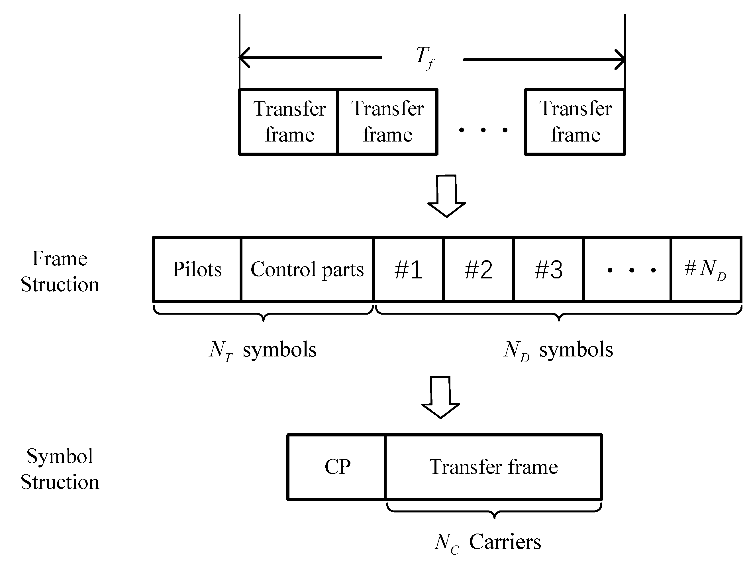
The transmitter is assumed to transmit on a per-frame basis, based on the IEEE 802.11a standard [20,21]. In every transmitted frame, there are symbols, where symbols are frequency-conducting and control symbols, and symbols are data symbols. frames can be transmitted during transmission duration , given that the length of time for transmitting an OFDM symbol is . In OFDM modulation, each symbol comprises NC sub-carriers, with 75% dedicated to data transmission and the other 25% used for pilot carriers, null sub-carriers, and guard bands to correct carrier frequency offset. In addition, a Cyclic Prefix (CP) is included in each symbol, making up 25% of the total number of sub-carriers in each symbol. Figure 6 illustrates the schematic diagram of the transmission frame and OFDM symbol structure.
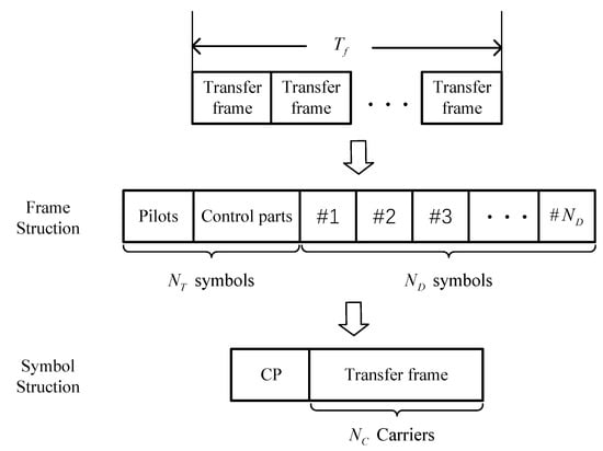
Figure 6.
Transmission frames and OFDM symbol structure.
The communication transmission rate is determined by the selection of [28]. The throughput of the sub-band i is as follows:
where the represents the number of transfer frame in .
Therefore, the overall throughput of the NC-OFDM system can be expressed as the sum of selected sub-band throughput:
2.2. FSMS Model
Rayleigh distribution is commonly used as a fading channel model in multipath propagation environments [29,30]. It was assumed that the signal fading at the receiver was distributed according to Rayleigh. The probability density function of the average received SNR under Rayleigh fading is given as follows [30]:
where represents the average received SNR.
Dividing the received SNR thresholds is the first step in establishing the model. It is assumed that the system always transmits at maximum available power, i.e., at a constant transmit power [26], and divide the entire SNR range into non-overlapping continuous intervals, where () is the quantization threshold. When the received SNR falls within the interval , the sub-band transmission rate corresponds to the rate in transmission mode k as per Table 1 ( referencing Table 1). To avoid deep channel fading, when , the sub-band rate .
To simplify the analysis, consistent with [22] Equation (3), the Packet Error Rate (PER) is approximated as:
where k is the transmission mode index, and are the corresponding parameters for mode k.
The boundary (i.e., switching threshold) of transmission mode k is set as the minimum SNR required to achieve the target PER. As expressed in [22] Equation (7), the threshold partitioning is:
Therefore, based on (3), (4), and Table 1 the probability of the sub-band transmission rate being in transmission mode k is given by:
In previous sections, the channel has been considered to be frequency flat. The FSMS model assumes state transitions occur only between two adjacent states [23]. By utilizing the Level Crossing Rate (LCR) of the wireless fading channel [31], the one-step transition probabilities of the Markov chain can be determined. Therefore, the transition probabilities between different states can be acquired as follows:
where represents the state of the channel and represents the LCR with threshold , reflecting the rate of change in the received signal over time. Under Rayleigh distribution, the expression of LCR can be found in [31] as follows:
where represents the maximum Doppler frequency, and represents the amplitude threshold of the signal.
In summary, the sub-band is modeled as a FSMS with a state transition matrix, which is banded as:
3. Problem Formulation
In this section, the problem of data transmission under channel fading and dynamic jamming is modeled as an MDP, with definitions provided for system states, actions, and rewards.
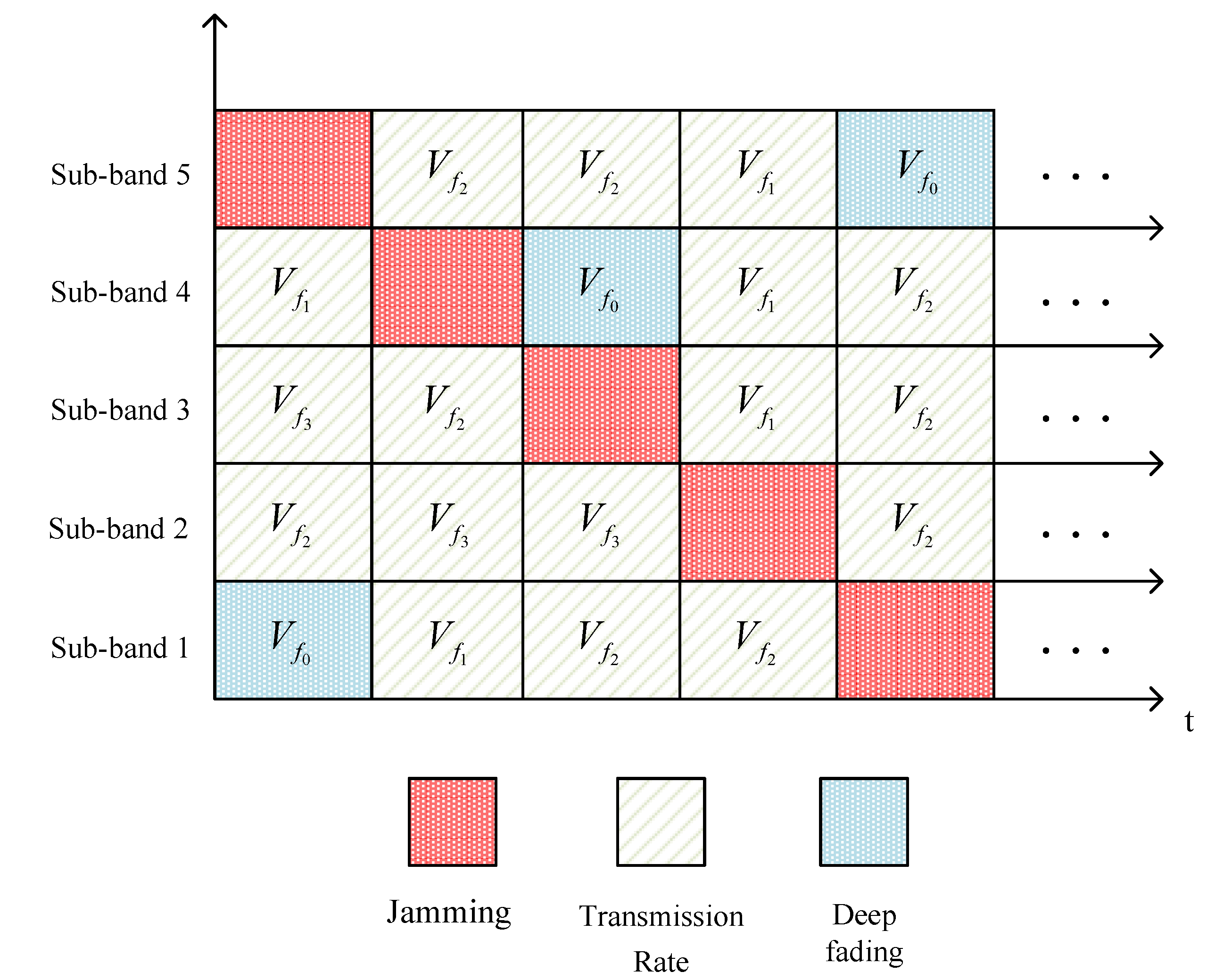
Figure 7 illustrates the relationship between interference and sub-band transmission rate variation when a jammer releases linear sweep jamming, given . The horizontal axis represents time, and the vertical axis denotes the sub-bands. In the current time slot, the sub-bands with jamming are marked with red squares, the green squares depict the changes in transmission rates over time across sub-bands, and the sub-bands in deep fading are represented by blue squares.

Figure 7.
Schematic diagram of jamming and sub-band rate variation.
It is essential to switch the transmission sub-band, considering that jammers could change the jamming sub-bands across various time slots. The transmission rate for each time slot is established by selecting the MCS corresponding to the chosen sub-band. It is worth noting that, in fading environments, the maximum transmission rate a sub-band can support may vary from one time slot to another. Choosing a higher MCS might degrade the communication quality due to pronounced fading of the selected sub-band, leading to data loss. On the other hand, opting for a lower MCS ensures communication reliability but may substantially diminish the communication throughput. As such, a careful selection of both the transmission sub-band and the MCS is vital to sidestep jamming and achieve optimal communication throughput. Given the challenges posed by fading and jamming, our primary aim is to determine the most effective transmission strategy (in terms of sub-band and rate) that boosts communication throughput while helping users elude jamming.
The wireless environment and user’s dynamic interactions in the optimization problem can be interpreted as a Markovian-based sequential decision-making process, modeled through an MDP [23]. The decision-making process for users in an unknown environment is represented as an MDP quadruple . The MDP provides the agent with a mathematical model, enabling the agent to seek the optimal strategy by solving the MDP.
(1) State : The environmental state characterizes system features. In Q-learning, the definition of should minimize redundant information to avoid interfering with the agent’s decision-making. In this paper, the state at time slot t is defined as =, , where represents the selected transmission sub-band in the current time slot, denotes the transmission rate of the chosen sub-band, and indicates the sub-band where jamming is present.
(2) Action : Action reflects responses to the environment with present state information. This paper defines the action space as a combination of all sub-band sets and transmission rate sets corresponding to MCS. Therefore, the action chosen by the user in time slot t under state is defined as:,, , .
(3) Transfer probability : When an action is executed by the agent, the subsequent state is influenced, establishing a relationship between neighboring states. The probability of transitioning from state to state after executing action is defined as:
where
represents the probability of transitioning to state after choosing action from state .
(4) Reward : After completing an action, the agent receives feedback from the environment, represented as a reward. The reward represents the optimization goal of the Q-learning task. In this paper, our goal is to avoid jamming and maximize the system throughput in a fading environment. The system’s throughput increases with a higher MCS level, meaning a greater data transmission rate.
Considering both jamming and fading have an impact on the success of data transmission, a transmission indicator function is defined as follows:
When the indicator function , it signifies successful communication, and the receiver acknowledges by sending back an ACK through the control channel. Conversely, when the indicator function , it indicates communication failure, prompting the receiver to send a NACK through the control channel.
Therefore, the immediate reward of the system is defined as:
In this paper, the goal is to maximize the throughput performance of NC-OFDM systems through online learning. At a given time slot, the action is related to the historical transmission strategy and historical utility . The set consisting of all feasible policies is denoted as , and the optimal selection policy defined as follows:
4. Reinforce Learning-Based Optimal Action Acquisition Scheme
4.1. Q-Learning Algorithm
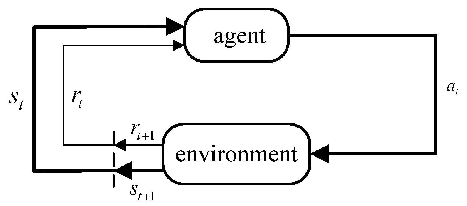
The process of reinforcement learning involves five key components: agent, environment, state, action, and reward. Figure 8 illustrates the schematic of this process. First, the agent interacts with the environment at time t to obtain the current state . Then, the agent selects an action at based on the behavioral policy, which impacts the environment. The environment offers immediate feedback as a reward to the agent’s action, and updates the state for the following iteration.
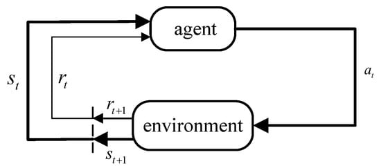
Figure 8.
Markov process of agent-environment interaction.
Q-learning is a classical and widely applicable reinforcement learning method that constructs a Q-value table to evaluate the performance of actions for each state–action combination [23]. The agent keeps a Q-table throughout the algorithm’s execution. At state, the user picks action , based on the current Q-value table , using a specific strategy, and earns an immediate reward , while transitioning to state , the Q-values in the current Q-value table are updated, resulting in an improved policy. The approach stabilizes following multiple iterations. The formula for updating the Q-values is as follows:
where represents the learning rate that modifies the Q-value corresponding to the current state–action combination during each iteration; is the discount factor, reflecting the influence of future rewards on the current action selection.
4.2. Modified Q-Learning Anti-Jamming Algorithm Based on Confidence Intervals
A crucial aspect of the Q-learning is the exploration and utilization of a balanced state–action set, which is worth noting. Over-reliance on the current can prevent adequate assessment of rewards for different state–action pairs, leading to a local optimum. Conversely, over-exploration can prevent convergence and finding the optimal policy. Q-learning generally uses or SoftMax policy to avoid the exploration–exploitation dilemma, but they only work for small state–action sets.
Unlike other studies based on Q-learning where the state–action set is small [16,23], in this paper, the size of the state–action set is denoted by . As increases, the state–action set expands, and normal Q-learning may not converge to the optimal Q-value.
The UCB algorithm, created for the multi-arm bandit problem, offers a technique to balance exploration and utilization. The UCB algorithm uses the UCB value to represent the upper confidence bound. The UCB value for each arm depends on two parts: the average reward of the currently selected arm and the confidence level , which represents the uncertainty in the action value estimate. The calculation for the UCB value of the ith arm is illustrated in (17):
where is the average reward of the ith arm, indicates the number of times the arm has been executed up to now, and c is a constant greater than 0 that controls the level of exploration. Confidence inclusion encourages the use of infrequently selected options and decreases the selection of actions with lower value estimates.
Drawing from the literature [18] and the UCB algorithm, a modified Q-learning anti-jamming algorithm based on confidence intervals is proposed. Instead of following the normal Q-learning method for calculating Q-values, the Q-values for all state–action combinations under the current state are updated in each process and a confidence term is included in the proposed approach. The proposed algorithm aims to balance the exploration–exploitation dilemma in Q-learning algorithm. The UCB-Q value for each state–action pair in state is defined as follows:
The confidence term in the formula represents the volatility of rewards, and its presence dynamically adjusts the exploration scope, helping to learn the optimal policy with minimal selection cost. The confidence definition in (17) was modified by incorporating rewards in a normalized form. As a result, the confidence term can be defined as:
where is the cumulative number of times action a has been executed at time t, and is the normalized reward for action a under state , which is calculated as follows:
The SoftMax policy is employed to guide action selection in this study. The action selection strategy of SoftMax is based on the Boltzmann distribution. Specifically, the update formula for the probability vector is given by:
where is the Boltzmann coefficient, and is the probability of choosing action at time .
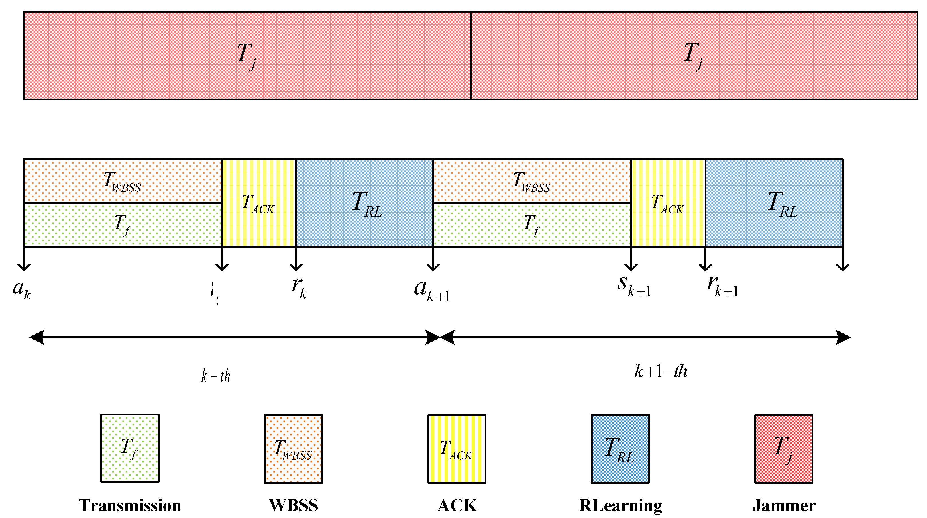
Figure 9 shows the time-slot for modified Q-learning algorithm. The time slot length for user transmission is designated as and for jamming. User follows a sequence of data transmission/broadband spectrum sensing (performed synchronously, ), ACK feedback, and reinforcement learning. The algorithm accomplishes one iteration during every communication time slot. Algorithm 1 provides the detailed process of the modified Q-learning algorithm.
| Algorithm 1 The modified Q-learning anti-jamming algorithm based on confidence intervals |
|
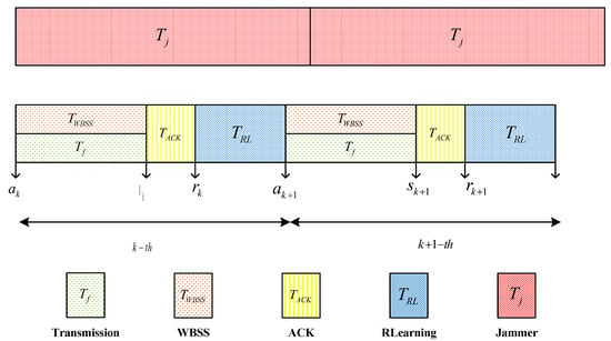
Figure 9.
The time-slot structure of the modified QL algorithm.
5. Simulation Results and Discussion
In this section, the simulation parameters for the NC-OFDM system and the proposed algorithm are presented. Additionally, its performance is validated through MATLAB simulation experiments.
5.1. Simulation Parameter
Based on the FSMS model established in Section 2, setting the average received SNR: = , target PER: = , Doppler shift: = 10 Hz, the set of sub-band transmission rate states can be obtained as (Mbps). Adaptive MCS technology is employed, where various information transmission rates are achieved through different combinations of modulation modes and coding efficiencies. With , the essential parameter settings are shown in Table 2. The specific NC-OFDM communication system and the simulation parameter settings of the proposed algorithm are shown in Table 3. The OFDM parameter settings are based on [32], and the time parameter settings are adjusted based on [23].
Table 2.
Convolutional coded based transmission modes and parameters for AMC communication.
Table 3.
Simulation parameters.
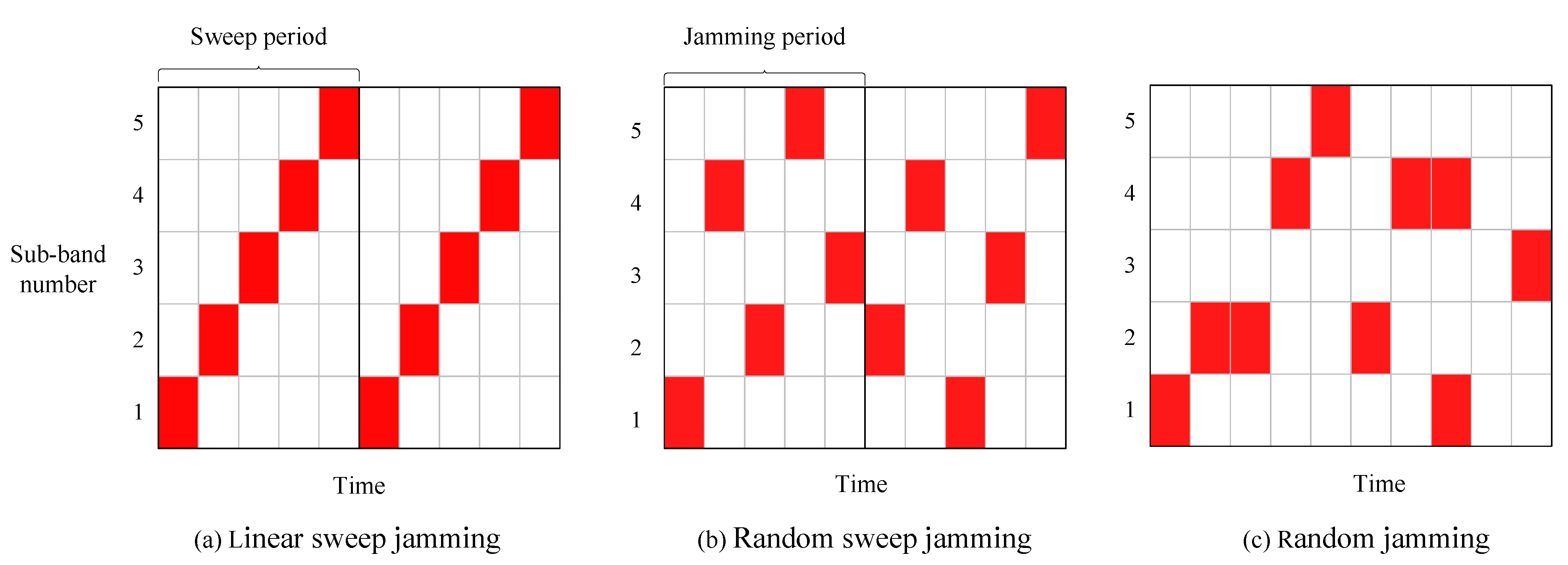
To confirm the performance of the proposed algorithm, simulations are conducted using linear sweep, random sweep, and random jamming methods. The three types of jamming patterns are separately illustrated in schematic diagrams Figure 10a–c. The red squares represent the sub-bands currently experiencing jamming. Specifically, random sweep jamming, which is based on linear sweep jamming, disrupts sub-bands in a random time–frequency pattern within each jamming cycle, while the random jamming occurs without any pattern.
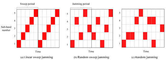
Figure 10.
Jamming pattern.
To evaluate the effectiveness of the proposed algorithm, its performance is compared to the following two transmission schemes:
- 1.
- Q-learning: The user adopts the standard Q-learning described in Section 4 as the execution algorithm and the Q-value is updated according to (16).
- 2.
- Perception-based random selection algorithm: Based on the WBSS results for the current time slot, the user randomly selects the non-interfered sub-band and transmission rate. This selection strategy is more intuitive.
Unless otherwise noted, the figures in this paper calculate each throughput point as the average throughput over 900 consecutive time slots.
5.2. Simulation Result
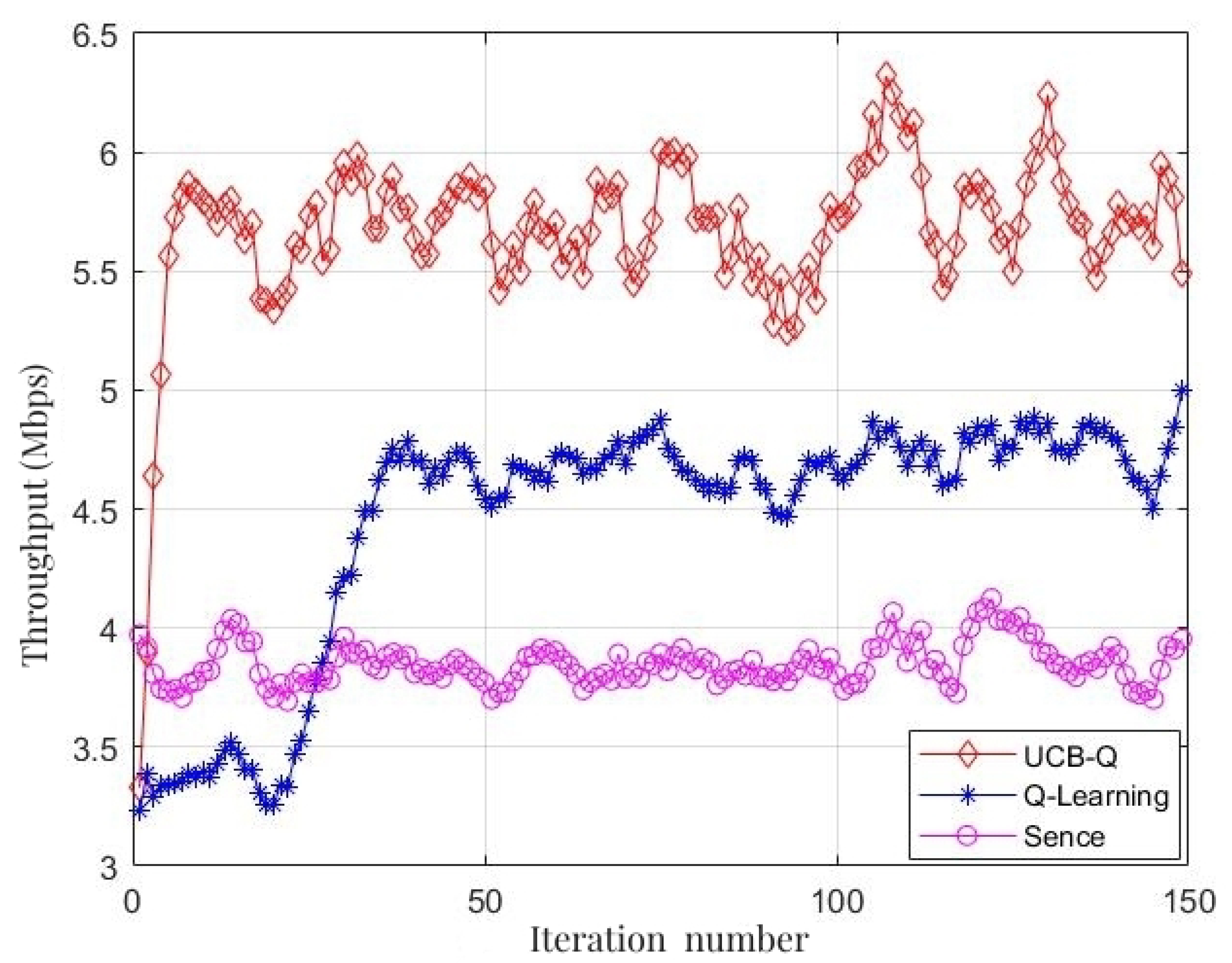
Figure 11, compares the throughput under three different algorithms. The simulation results show that the communication strategy, which using the perception-based random selection algorithm, has the lowest throughput, which is around 3.7 Mbps. With the aid of the Q-learning algorithm, the Q-learning-based communication strategy can respond to external environmental changes and learn from them. It eventually converges to a throughput of about 4.6 Mbps, marking a 24.32% enhancement over the perception-based algorithm. Meanwhile, the communication strategy based on the proposed algorithm can quickly learn the optimal transmission policy in a complex environment with both jamming and fading. The throughput converges at 5.75 Mbps, which is a 25% improvement over the Q-learning algorithm and a 55.41% improvement over the perception-based random selection algorithm, clearly outperforming the other two strategies.
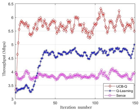
Figure 11.
Throughput comparison of different algorithm.
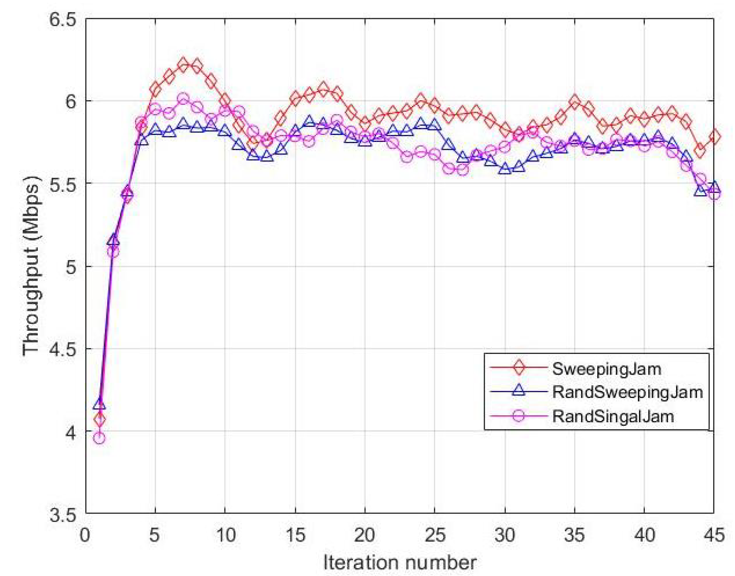
By not requiring prior knowledge about jamming, the modified Q-learning algorithm based on confidence intervals can explore and learn patterns in unknown jamming environments, making it adaptable to various dynamic jamming conditions. Figure 12, illustrates the throughput performance of the proposed algorithm during the three types of jamming mentioned earlier. In all three dynamic jamming types, the system’s throughput improves and eventually stabilizes, showing strong anti-jamming capabilities. Specifically, under linear sweep jamming, the throughput is maximized to 5.9 Mbps, while the throughput under random sweep jamming and random jamming is similar, settling at around 5.7 Mbps. The result is because of the simple jamming pattern of linear sweep jamming, which makes it easier for the algorithm to learn and adjust to its features.
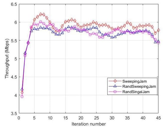
Figure 12.
Throughput comparison of different jamming types.
Figure 13 shows how the exploration factor c affects the reward values. The points in the figure represent an average of 500 consecutive iterations. It is clear from the simulation results that the proposed algorithm converges to the slowest and attains the lowest reward value upon convergence when c = 0. The worst performance occurs when c = 0 since the algorithm reverts to the normal Q-learning and faces the ’exploration–exploitation’ dilemma. When c increases, there is an improvement in both the speed of convergence and the final reward values. The algorithm reaches its fastest convergence and highest reward value when c = 2.5, balancing exploration and exploitation. Although the convergence is faster at c = 3 than c = 0, the final reward value is almost the same and significantly lower than c = 2.5. The algorithm’s drop in performance is due to excessive exploration caused by increasing exploration factor c, leading to faster convergence but preventing optimal policy learning.
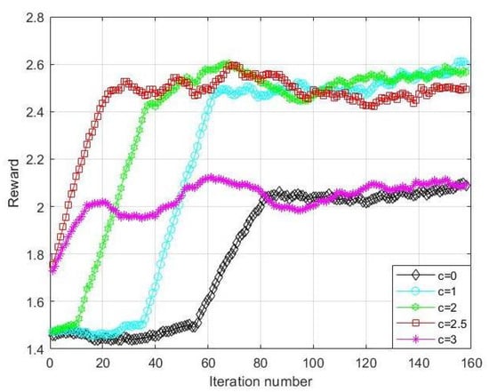
Figure 13.
Impact of exploration factor c on reward value.
6. Conclusions
In this paper, the transmission parameter selection in OFDM systems with time-varying fading and jamming is studied. First, to describe the time-varying features of the fading channel, an FSMS model was created based on changes in transmission rate. Subsequent analysis of the state transitions in the problem led to its formulation as an MDP. To address the exploration–exploitation dilemma induced by the vast state–action space, a modified Q-learning anti-jamming algorithm based on confidence intervals was proposed. Simulation results have proved that the proposed algorithm converges more rapidly and achieves higher throughput compared to traditional Q-learning and sensing-based algorithms. Additionally, the suggested algorithm performed well in multiple dynamic jamming scenarios.
Author Contributions
Methodology, L.Y. and X.Y.; Software, X.Y. and Y.X.; Writing—original draft, X.Y.; Writing—review & editing, L.Y., Y.L., Y.X. and Y.S.; Funding acquisition, Y.L. All authors have read and agreed to the published version of the manuscript.
Funding
This research was funded by National Natural Science Foundation of China: 62071488.
Data Availability Statement
Due to institutional data privacy requirements, our data is unavailable.
Conflicts of Interest
The authors declare no conflict of interest.
References
- Yao, F.Q.; Zhang, Y.; Liu, Y.X. Security and control for electromagnetic spectrum. J. Command Control 2015, 1, 278–283. [Google Scholar]
- Pelechrinis, K.; Iliofotou, M.; Krishnamurthy, S.V. Denial of service attacks in wireless networks: The case of jammers. IEEE Commun. Surv. Tutor. 2010, 13, 245–257. [Google Scholar] [CrossRef]
- Rajbanshi, R.; Wyglinski, A.M.; Minden, G.J. An efficient implementation of NC-OFDM transceivers for cognitive radios. In Proceedings of the 2006 1st International Conference on Cognitive Radio Oriented Wireless Networks and Communications, Mykonos, Greece, 8–10 June 2006; pp. 1–5. [Google Scholar]
- Bahai, A.R.S.; Saltzberg, B.R.; Ergen, M. Multi-Carrier Digital Communications: Theory and Applications of OFDM; Springer: New York, NY, USA, 2004; ISBN 9780387225753. [Google Scholar]
- Xu, G.; Zhu, Y.; Han, M. Broadband cognitive radio transmission based on sub-channel sensing and NC-OFDM. Int. J. Commun. Netw. Inf. Secur. 2010, 2, 98. [Google Scholar]
- Grover, K.; Lim, A.; Yang, Q. Jamming and anti–jamming techniques in wireless networks: A survey. Int. J. Ad Hoc Ubiquitous Comput. 2014, 17, 197–215. [Google Scholar] [CrossRef]
- Sun, W.; Amin, M.G. A self-coherence anti-jamming GPS receiver. IEEE Trans. Signal Process. 2005, 53, 3910–3915. [Google Scholar] [CrossRef]
- Song, K.-B.; Ekbal, A.; Chung, S.T.; Cioffi, J.M. Adaptive modulation and coding (AMC) for bit-interleaved coded OFDM (BIC-OFDM). IEEE Trans. Wirel. Commun. 2006, 5, 1685–1694. [Google Scholar] [CrossRef]
- Choi, J.W.; Lee, Y.H. Improved AMC using adaptive SIR thresholds in OFDM based wireless systems. In Proceedings of the IEEE Wireless Communications and Networking Conference, 2006. WCNC 2006, Las Vegas, NV, USA, 3–6 April 2006; Volume 3, pp. 1289–1292. [Google Scholar]
- Bolcskei, H. MIMO-OFDM wireless systems: Basics, perspectives, and challenges. IEEE Wirel. Commun. 2006, 13, 31–37. [Google Scholar]
- Patil, P.; Patil, M.R.; Itraj, S.; Bomble, U.L. A review on MIMO OFDM technology basics and more. In Proceedings of the 2017 International Conference on Current Trends in Computer, Electrical, Electronics and Communication (CTCEEC), Mysore, India, 8–9 September 2017; pp. 119–124. [Google Scholar]
- Yang, Y.; Zhang, Q.; Wang, Y.; Emoto, T.; Akutagawa, M.; Konaka, S. Adaptive resources allocation algorithm based on modified PSO for cognitive radio system. China Commun. 2019, 16, 83–92. [Google Scholar] [CrossRef]
- Demirci, S.; Gözüpek, D. Switching cost-aware joint frequency assignment and scheduling for industrial cognitive radio networks. IEEE Trans. Ind. Inform. 2019, 16, 4365–4377. [Google Scholar] [CrossRef]
- Rang, Y.; Chen, D.; Cheng, Y.; Wang, X. Cognitive anti-jamming intelligent decision based on improved artificial bee colony algorithm. J. Signal Process. 2019, 35, 240–249. [Google Scholar]
- Liang, Y.; Tan, J.; Niyato, D. Overview on intelligent wireless communication technology. J. Commun. 2020, 41, 1–17. [Google Scholar]
- Machuzak, S.; Jayaweera, S.K. Reinforcement learning based anti-jamming with wideband autonomous cognitive radios. In Proceedings of the 2016 IEEE/CIC International Conference on Communications in China (ICCC), Chengdu, China, 27–29 July 2016; pp. 1–5. [Google Scholar]
- Bkassiny, M.; Li, Y.; Jayaweera, S.K. A survey on machine-learning techniques in cognitive radios. IEEE Commun. Surv. Tutor. 2012, 15, 1136–1159. [Google Scholar] [CrossRef]
- Moy, C. Reinforcement learning real experiments for opportunistic spectrum access. In Proceedings of the WSR’14, Karlsruhe, Germany, 14 March 2014; p. 10. [Google Scholar]
- Chung, S.T.; Goldsmith, A.J. Degrees of freedom in adaptive modulation: A unified view. IEEE Trans. Commun. 2001, 49, 1561–1571. [Google Scholar] [CrossRef]
- Physical Layer Aspects of UTRA High Speed Downlink Packet Access. Tech. Rep. 3GPP TR 25.848 v4. 0.0. 2005. Available online: https://portal.3gpp.org/desktopmodules/Specifications/SpecificationDetails.aspx?specificationId=1281(accessed on 3 September 2023).
- Doufexi, A.; Armour, S.; Butler, M.; Nix, A.; Bull, D.; McGeehan, J.; Karlsson, P. A comparison of the HIPERLAN/2 and IEEE 802.11 a wireless LAN standards. IEEE Commun. Mag. 2002, 40, 172–180. [Google Scholar] [CrossRef]
- Liu, Q.; Zhou, S.; Giannakis, G.B. Queuing with adaptive modulation and coding over wireless links: Cross-layer analysis and design. IEEE Trans. Wirel. Commun. 2005, 4, 1142–1153. [Google Scholar]
- Kong, L.; Xu, Y.; Zhang, Y.; Pei, X.; Ke, M.; Wang, X.; Bai, W.; Feng, Z. A reinforcement learning approach for dynamic spectrum anti-jamming in fading environment. In Proceedings of the 2018 IEEE 18th International Conference on Communication Technology (ICCT), Chongqing, China, 8–11 October 2018; pp. 51–58. [Google Scholar]
- Pimentel, C.; Falk, T.H.; Lisbôa, L. Finite-state Markov modeling of correlated Rician-fading channels. IEEE Trans. Veh. Technol. 2004, 53, 1491–1501. [Google Scholar] [CrossRef]
- Zhang, Q.; Kassam, S.A. Finite-state Markov model for Rayleigh fading channels. IEEE Trans. Commun. 1999, 47, 1688–1692. [Google Scholar] [CrossRef]
- Alouini, M.S.; Goldsmith, A.J. Adaptive modulation over Nakagami fading channels. Wirel. Pers. Commun. 2000, 13, 119–143. [Google Scholar] [CrossRef]
- Wang, H.S.; Moayeri, N. Modeling, capacity, and joint source/channel coding for Rayleigh fading channels. In Proceedings of the IEEE 43rd Vehicular Technology Conference, Secaucus, NJ, USA, 18–20 May 1993; pp. 473–479. [Google Scholar]
- Razavilar, J.; Liu, K.R.; Marcus, S.I. Jointly optimized bit-rate/delay control policy for wireless packet networks with fading channels. IEEE Trans. Commun. 2002, 50, 484–494. [Google Scholar] [CrossRef]
- Kong, H.; Shwedyk, E. Markov characterization of frequency selective Rayleigh fading channels. In Proceedings of the IEEE Pacific Rim Conference on Communications, Computers, and Signal Processing, Victoria, BC, Canada, 17–19 May 1995; pp. 359–362. [Google Scholar]
- Park, J.M.; Hwang, G.U. Mathematical modeling of Rayleigh fading channels based on finite state Markov chains. IEEE Commun. Lett. 2009, 13, 764–766. [Google Scholar] [CrossRef]
- Sutton, P.D.; Nolan, K.E.; Doyle, L.E. Cyclostationary signatures in practical cognitive radio applications. IEEE J. Sel. Areas Commun. 2008, 26, 13–24. [Google Scholar] [CrossRef]
- Jones, A.M.; Headley, W.C. Considerations of Reinforcement Learning within Real-Time Wireless Communication Systems. In Proceedings of the MILCOM 2022–2022 IEEE Military Communications Conference (MILCOM), Rockville, MD, USA, 28 November–2 December 2022; pp. 418–425. [Google Scholar]


Disclaimer/Publisher’s Note: The statements, opinions and data contained in all publications are solely those of the individual author(s) and contributor(s) and not of MDPI and/or the editor(s). MDPI and/or the editor(s) disclaim responsibility for any injury to people or property resulting from any ideas, methods, instructions or products referred to in the content. |
© 2023 by the authors. Licensee MDPI, Basel, Switzerland. This article is an open access article distributed under the terms and conditions of the Creative Commons Attribution (CC BY) license (https://creativecommons.org/licenses/by/4.0/).