Measuring Received Signal Strength of UWB Chaotic Radio Pulses for Ranging and Positioning

Abstract

The use of ultra-wideband (UWB) signals for local positioning is very attractive for practice, because such signals have the potential to provide centimeter precision. In this paper, we consider wireless ranging (distance measurement) and positioning, using one of the kinds of UWB signals, i.e., chaotic radio pulses, which are noise-like signals with no constant shape. The distance measurement is based on an assessment in the receiver of the power of UWB chaotic radio pulses emitted by the transmitter. A new method for estimating their power and its experimental implementation is proposed and described. Experimental layouts of the transmitter and receiver and the principles of their operation are described. To determine the main features of this method under real signal propagation conditions, full-scale indoor measurements were carried out, and statistical estimates of the accuracy were made. We present the results of experimental testing of the proposed approach for positioning the emitter relative to a system of anchors in an office space 6 × 6.5 m² in the mode of measuring object coordinates on a line and on a plane. The mean absolute error (MAE) of distance measurement (1D) was 25 cm, and the root mean squared error (RMSE) was 39 cm. When positioning on a plane (2D), the MAE of coordinate estimation was 34 cm and the RMSE was 42 cm. The proposed distance measurement method is intended for use in wireless UWB transceivers used in wireless sensor networks.

1. Introduction

The wireless positioning of objects indoors, where global navigation satellite systems (GNSSs) are not accessible, plays an important role in the development of modern technologies, industrial automation, and the provision of customer services. The importance and relevance of this problem is confirmed by hundreds of publications. The rapid development of this area has already led to the emergence of a wide variety of technologies and methods, the purpose of which is to measure the distance between objects as accurately as possible and position them in space. To solve this problem, various types of signals (sound, light, radio waves) are proposed, among which the most convenient from a technical point of view are radio systems due to their omnidirectional and high penetrating ability [1,2]. In the development of advanced radio communication systems (6G, etc.), stake has been placed in radio positioning systems [3].

Positioning is a complex problem that must be addressed at several levels:

• Development of radio technology at the physical layer. This includes the study of various signal characteristics (frequency, time, correlation, energy) and the ways they can be used to measure distance. One of the important aspects of radio technology is that it can be used for both positioning and data transmission, i.e., the distance can be measured by the same equipment with which the information is delivered, or both tasks can be processed simultaneously. To date, WiFi, Bluetooth, ZigBee, and UWB technologies are the most popular among the radio technologies used for positioning.
• Signal characteristic used for positioning. Commonly used approaches are estimation by the received signal strength (RSS), time of arrival (TOA), time difference of arrival (TDOA), and angle of arrival (AOA). The choice of the method depends on the specific technology, the available equipment, and the ability to implement one or another method.
• Positioning method. Positioning methods are divided into two groups: one based on a preliminary distance measurement (ranging based) and the other based on the statistical accumulation of a database of received signal characteristics at different points in space, with further probabilistic determination of object position and comparing of the signal characteristics with a database (fingerprinting).
• Signal post-processing methods that improve the accuracy of coordinate estimates. Approaches based on Kalman filtering [4,5], particle filters, machine learning methods [6], neural networks [7,8,9], as well as hybrid (fusion) approaches, based on combinations of different technologies or different distance measurement methods, are proposed [5,10].

For this paper, we focused on the design and research of the positioning problem at the physical layer—the radio signal layer. The performance of various radio technologies, their benefits, and their drawbacks are widely discussed in scientific periodicals. A critical review of modern technologies that can be applied to 3D positioning—such as WiFi, Bluetooth, UWB, mmWave, visible light, and sound-based technologies—their performance, and their weak and strong points, is given in [1]. The authors of [11] focused on the technologies used in the Internet-of-Things. In [2], the stress was put on industrial positioning applications, whereas [12] provided an overview of the state of the art in academic research of low-cost, low-power engineering solutions that can provide centimeter accuracy.

The mentioned works show that characteristic positioning accuracy varies for Wi-Fi within ∼1–3 m, for Bluetooth within ∼2–5 m, for RFID within ∼2 m, for ZigBee within ∼3–5 m, and for UWB within ∼0.1–0.5 m. To date, UWB-based technologies are the only class of radio systems that consistently demonstrate centimeter accuracy in real wireless channels due to the enhanced radio signal bandwidth.

Mass research on license-free UWB solutions started with the introduction of the US FCC spectral mask [13,14] and the subsequent development of a number of international standards for UWB wireless communications, such as IEEE 802.15.3a [15,16] (ultimately not adopted), IEEE 802.15.4a (wireless sensor networks) [17], IEEE 802.15.6 (wireless body area networks) [18], and IEEE 802.15.4z [19,20,21]. The ultra-wide frequency range can potentially provide both high data rates and high positioning accuracy—the latter feature being necessarily included in the above standards to ensure the positioning of the wireless sensor nodes. The integration of communication capabilities with object localization in space, the increase in operation frequencies, and the expansion of the frequency band are also emphasized in the next-generation communications [3,22].

The practical relation between the UWB frequency band and the distance measurement accuracy was considered for ultrashort pulses (USPs) in [23]. An experiment on 3D positioning and propagation time (TOA) measurements using UWB ultrashort pulses was described in [24]. The effect of the pulse shape on the positioning accuracy was studied, and an accuracy of 2–3 cm was achieved at a frequency bandwidth of 5 GHz. Experiments with a commercial Pozyx platform were described in [25], in which ultrashort pulses were used to measure TOA and to obtain positioning accuracy of 10 to 32 cm, using trilateration. A distance measurement method based on Acam’s TDC-GP2 chip that can measure 50 ps delays was described in [26]. With a frequency bandwidth of 1 GHz (a USP duration of about 1 ns) in the 5.6 GHz band, an accuracy of 40 cm at 30 m was obtained. In UWB radar-type systems [27], accuracy up to 0.5 cm was demonstrated. Special reviews on UWB technologies in positioning are given in [28,29,30].

From the theoretical point of view, the best accuracy by increasing the bandwidth can potentially be achieved when measuring the distance by the signal propagation time. However, this is not always the case in real wireless communication channels due to a possibly large dispersion of the pulse arrival time at the reception point as a result of multipath propagation [31,32]. In this regard, the benefits of measuring the propagation time compared to measuring the power of UWB signals is not obvious. Therefore, there are a significant number of papers that investigate the problem of measuring the power of UWB signals in order to estimate the distance between the transmitter and receiver and to position an object. Naturally, the RSS measurement and the related approaches to positioning have long been fruitfully discussed in the context of narrowband systems, the problems of which serve as an additional motivation for switching to UWB systems, and it would be reasonable to apply approaches and methods that have proven themselves in narrowband systems to UWB systems.

An overview of the methods for estimating distance by RSS measurements is given in [33]. The main approaches and problems that arise in this case have been analyzed with an emphasis on the TmoteSky, TelosB, MicaZ, and Imote2 motes, which are related to the IEEE 802.15.4 standard [34]. The data of specific measurements were presented. An important conclusion was that the localization error grew linearly from 20 cm at 1 m to 4–6 m at 20 m.

Various machine learning algorithms used to improve the accuracy of RSSI measurements were compared in [35]. Factors affecting 2D positioning accuracy for RSS fingerprinting systems were discussed in [36]. The above analytical data showed that despite the use of complex machine and deep learning algorithms, the positioning accuracy in narrowband systems based on RSS (RSSI) measurement usually did not exceed 1 m.

Measuring the received signal strength of UWB signals was also used to solve the problems of measuring distance and positioning. For example, ref. [37] explored the use of RSS to measure distance and to position objects with UWB ultrashort pulses. The performance of such a system was tested by UWB measurements in an indoor line-of-sight (LOS) scenario. As well as for narrowband systems, the distance measurement error depended on the measured distance. For 90% of measurements, the error was shown to be less than 1.5 m. An UWB distance measurement method based on the statistics of the power of the first beam was proposed in [38]. The dependence of the measurement results on the signal bandwidth was analyzed for the proposed approach. The authors of [39] addressed the problem of improving the distance measurement accuracy using the RSS characteristics of UWB ultrashort pulses: several machine learning methods were compared for a distance measurement problem. The best accuracy achieved when measuring the distance under the same conditions in which the system was trained was 2.1 cm. When measuring in other conditions, the accuracy amounted to 24 cm. UWB RSS measurements were applied to search a car in the parking lot in [40] and in [41] to localize the capsule in the human body in capsule endoscopy.

The authors of [42] used RSS measurements of the UWB multiband OFDM signal for positioning using the fingerprinting approach. The results of positioning experiments in a small network (1.76 × 2.0 m²) showed the accuracy of the root mean square error (RMSE) estimation of about 0.33 m.

We have mentioned certain papers, in which UWB RSS was used for positioning, but in most cases, it was applied in combination with other methods: either as power and time measurements using the same technology or in combination with other technologies, such as WiFi. There were methods that used UWB signals to locate sensors by measuring RSS [43] in an emission source localization problem. A combined approach complementing WiFi RSS fingerprinting with UWB RSS measurements and using a neural network was proposed in [44]. This approach allowed the authors to improve the positioning accuracy to 0.66 m.

One type of UWB signals is chaotic radio pulses, which are not as common as ultrashort pulses but are of interest from the viewpoint of the signal propagation physics and technical applications, in particular, in the problems of data transmission and wireless positioning.

This UWB signal has a noise-like waveform, a wide power spectrum, and a narrow autocorrelation function. The duration of a chaotic radio pulse can vary over a wide range without any effect on the signal bandwidth, which is completely determined by the properties of the dynamic system, i.e., the generator of the chaotic oscillations. This is an extremely useful property in a multipath environment. Since the pulse duration can be made much longer than the multipath response of the channel, the pulse power can be reliably estimated from the pulse envelope using a relatively low sampling rate.

Examples of the use of chaotic signals for distance measurement are presented mainly by radar-type systems. A method for determining distance in the ultrasonic range using chaotic signals was described in [45]. Distance measurement with a sonic system based on chaotic signals was also described in [46]. The approach proposed here was developed in [47], where a 2.4 GHz system for measuring the distance was proposed. An UWB microwave-photonic chaotic radar system for remote ranging was proposed in [48]. Note also a radar that used chaotic positional modulation [49], and a direct-chaotic radar was proposed in [50].

A distance measurement system using an incoherent receiver of chaotic signals was considered in [51], and its performance in real conditions was estimated experimentally. It used a time measurement technique (TWR, Two-Way Ranging) and a Fuzzy Logic algorithm to reduce the effect of NLOS (No Line-of-Sight) conditions.

In the existing equipment [52,53,54], chaotic radio pulses have been used to transmit information, so it is practically interesting to create a distance measurement method that could be a part of the process of wireless data exchange between the devices.

Earlier, in a number of experimental studies, fundamental questions were considered about the advisability of UWB chaotic signals in the schemes based on measuring the power level [55,56] or the propagation time [57] of chaotic radio pulses. The systems based on chaotic radio pulses were shown to have a potential for positioning.

The prospects for the successful use of chaotic radio pulses for positioning are also based on the results of a study of the conditions for the indoor propagation of chaotic radio pulses [58,59], during which patterns of signal power variation were revealed, and this kind of signal was shown to be free from small-scale fading; therefore, it makes sense to develop a system that would form the basis for a technically simple indoor ranging system.

As we have mentioned, there are a number of works on the use of chaotic signals for wireless distance measurement; however, this issue is still not well studied.

This paper is intended to fill this gap in the study of the possibilities of UWB chaotic signals for ranging and positioning. Here, we only focus on measuring distance by analyzing RSS.

The authors see the following reasons why the measurement of the chaotic signal RSS seems appropriate as a physical ground for positioning:

• UWB chaotic signals are used for both communication and positioning. In this case, the RSS measurement can be combined with the processes of transmitting/receiving data.
• Noise-like UWB signals are much less prone to multipath fading than narrowband signals, which means less power fluctuation or, other conditions being equal, fewer measurements to achieve the same accuracy as narrowband systems.
• Positioning based on time measurements can be combined with RSS measurements and they can complement each other, similar to the above schemes combining Wi-Fi and UWB systems.

The purpose and novelty of this study include the following:

• Development of a method for measuring the power of UWB chaotic radio pulses;
• Assessment of signal strength and distance measurement accuracy achievable by this method;
• Experimental verification of the proposed method in the problem of wireless ranging and positioning in a real indoor wireless channel;
• Thereby creating a baseline for the further development of approaches to solving the problem of wireless positioning of objects using UWB chaotic signals.

The paper is organized as follows. Section 2 describes the measurement method, signal type, signal modulation method, layout and measurement scenarios; the achievable power and distance accuracies are estimated theoretically. Section 3 contains the experimental data obtained during the measurements and the data analysis. In Section 4, the prospects of the proposed approach are discussed. Appendix A summarizes the symbol definitions used in the paper.

2. Methods and Materials

The paper investigates a method for wireless ranging and positioning using UWB chaotic radio pulses; the method is based on measuring the power of UWB chaotic radio pulses emitted by a transmitter (a target) and acquired by receivers (anchors) whose coordinates are known.

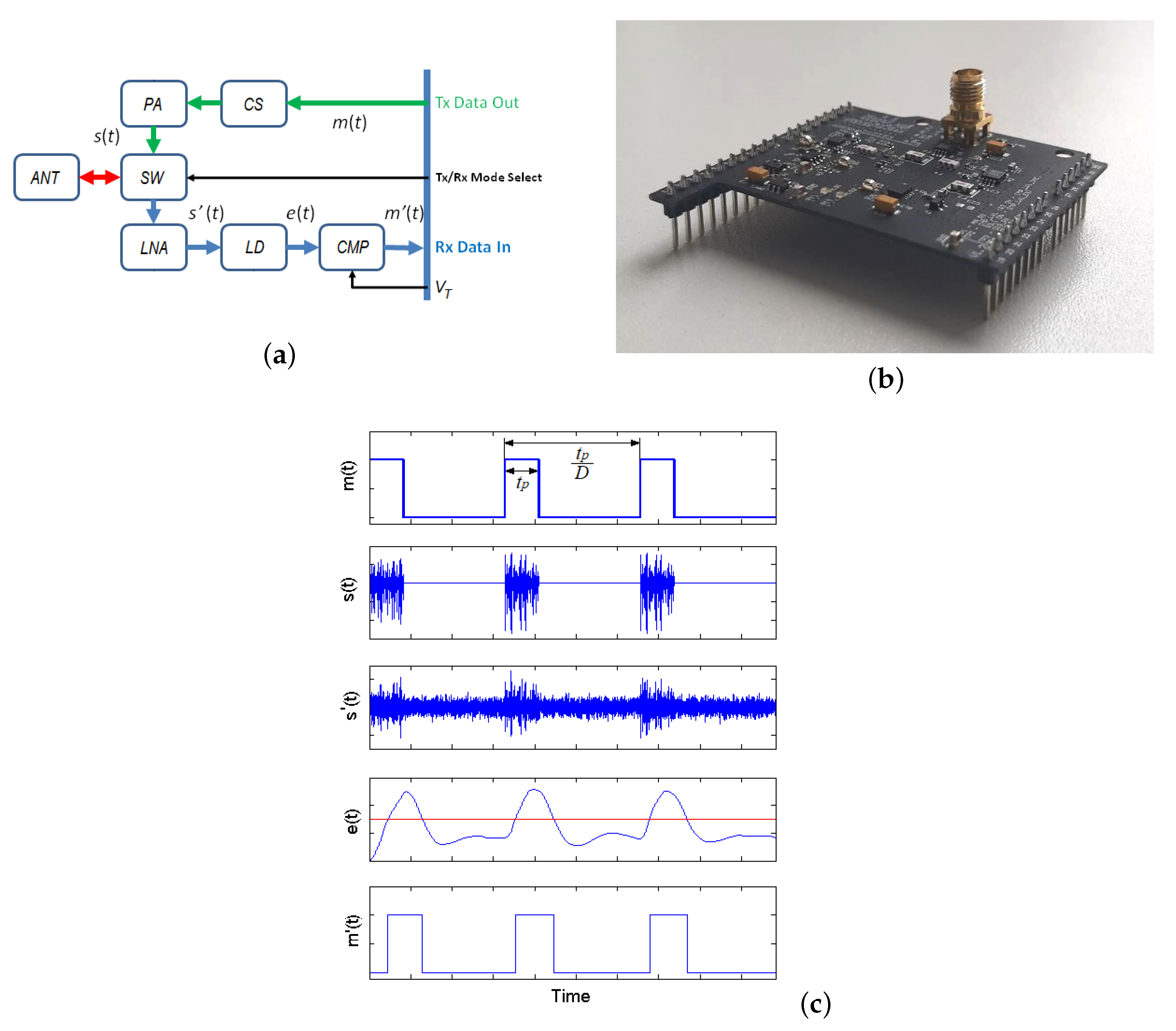
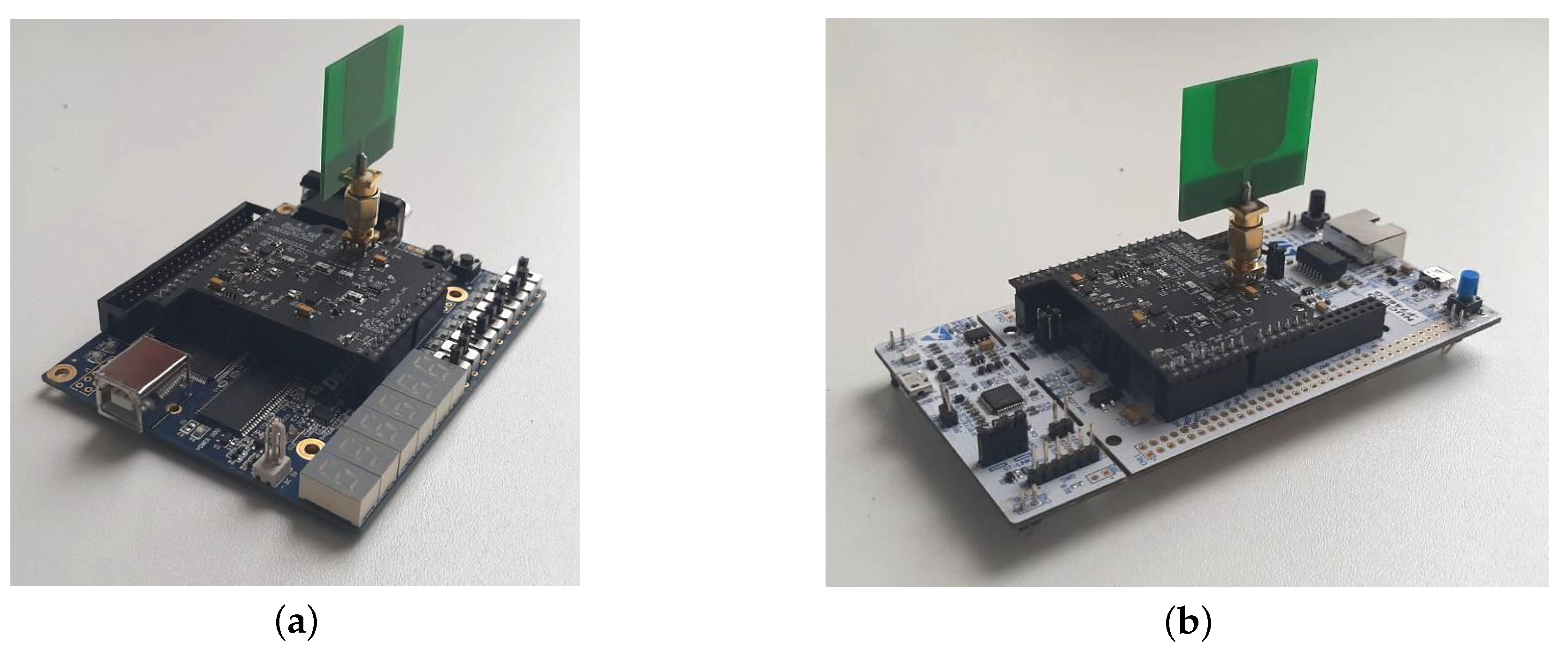
2.1. Wireless UWB Transceivers

In this paper, to solve the problem of ranging and positioning, we use microwave transceivers based on UWB chaotic radio pulses [52,53,54]. The transceivers are UWB modules (Figure 1) that are mounted on development boards with either an FPGA (target) or an MCU (anchor). All boards are equipped with an ST Morpho Connector. The block diagram of the UWB module is given in Figure 1a, and its layout is shown in Figure 1b. The module is an RF front-end device consisting of transmitting (Tx) and receiving (Rx) parts. The module (Figure 1a) is composed of a chaotic signal generator ($CS$), a power amplifier ($PA$), a switch ($SW$), an antenna ($ANT$), a low-noise amplifier ($LNA$), a log detector ($LD$), and a comparator ($CMP$). The module has two-level control inputs/outputs, which control the UWB chaotic signal modulation, emission, reception, and data exchange with an external device.

In general, this system implements the principle of direct chaotic communications (DCC) [52,53], which uses UWB chaotic radio pulses as a carrier.

A single-transistor generator on a bipolar transistor is used as a source of chaotic signal [60]. The chaotic generator ($CS$) with a power amplifier $\left(PA\right)$ continuously produces a UWB noise-like signal in the frequency band 3…5 GHz with the power spectrum in Figure 2. The output power of the unmodulated chaotic signal is $P_{Tx}$ = $12.5$ dBm.

The frequency range 3…5 GHz is permitted for unlicensed use in UWB systems [13,14], including positioning tasks. The average wavelength in this range is ∼ 7.7 cm. This frequency range has a good penetrating ability, and at the same time, the wavelength is large enough to experience no significant scattering by indoor propagation. Moreover, such a wavelength can provide good resolution when measuring distance by signal propagation time.

The chaotic signal is modulated by a stream of video pulses $m\left(t\right)$ using 2-position amplitude keying, while the pulse duration $t_P=0.625$ μs, duty cycle $D=1/2$, and pulse position duration $t_P/D=$1.25 μs. The modulated signal at the output of the transmitter is emitted in the communication channel by an UWB antenna $\left(ANT\right)$.

Typical signal waveforms at various circuit points are shown in Figure 1c.

In the receiving part, the stream of UWB chaotic radio pulses is received by the antenna $\left(ANT\right)$, amplified by a low-noise amplifier $\left(LNA\right)$, and detected by a log detector $\left(LD\right)$ (energy detector), i.e., the stream of chaotic radio pulses is retrieved in the analog form $\left(e\right(t\left)\right)$, and by comparing it with the threshold voltage $\left(V_T\right)$ in the comparator $\left(CMP\right)$, it is converted into a 2-level analog signal $m^{\prime }\left(t\right)$. Then, this 2-level signal is digitally processed on the development boards.

The emitter of chaotic radio pulses (the node whose coordinates are to be determined) is implemented on a DE10-Lite FPGA development board (Figure 3a). In the transmission mode, the UWB module under the control of the DE10-Lite board generates and emits a sequence of chaotic radio pulses. The FPGA allows us to form pulses with a very stable period and duty cycle.

The receivers of chaotic radio pulses (anchors) are implemented on STM32 Nucleo-F746ZG development boards (Figure 3b).

In the receiving mode, the UWB module (controlled by the STM32 Nucleo-F746ZG board) receives chaotic pulses and converts them into a 2-level signal in a $CMP$ comparator. The comparator compares the instantaneous value of the envelope $e\left(t\right)$ with the threshold voltage $V_T$, which is synthesized by a 12-bit DAC on the board from an integer value T of the range [0, 4095] that is put in the DAC.

The $ANT$ antenna is an external UWB 3.1...10.6 GHz antenna, which is connected to the module with an SMA connector. The antenna is a printed dipole with a toroidal radiation pattern (omnidirectional in the XY plane). The antenna parameters are given in [61] (“generic antenna”). A photo of the antenna, the calculated radiation patterns, and the experimentally measured S11 parameter are given in the Supplementary Materials.

2.2. Method of Measuring Signal Power

When measuring distance by the received signal strength, we imply the following [33]:

• The measured value of the received signal power can unambiguously be related to the actual received signal power;
• The received signal power decreases with the distance d to the source in accordance with a monotonic deterministic law.

In this paper, the signal power at the reception point is measured with a log detector [62], which is a part of the module, that gives an output signal, the amplitude A of which is proportional to the microwave signal power P at its input.

A change in the amplitude $\Delta A=A_1-A_2$ of the signal at the output of the log detector is proportional to the change in power (in dB) at its input $\Delta P=P_1-P_2$:

$$\Delta A=h\Delta P$$

(1)

where h is the slope of the log detector. Therefore, in order to estimate the change in the signal power at the input of the log detector, we measure the change in the signal amplitude at the output of the detector.

The instantaneous power value measured by the receiver, as well as the corresponding instantaneous value of the voltage amplitude $e\left(t\right)$, is a random variable, which is determined by the power of the emitted chaotic signal and the effects of signal propagation over the radio channel (multipath propagation, interference from third-party radio systems, movement in the room, imperfection of the input circuits of the receiver). In addition, the amplitude of the chaotic signal $s\left(t\right)$ is not constant; therefore, the envelope of the chaotic signal in the receiver $e\left(t\right)$ has a complex, irregular shape (Figure 4).

Thus, we need a statistical rule to evaluate the power of the chaotic radio pulses from the instantaneous values of the observed envelope $e\left(t\right)$, i.e., to estimate of amplitude of the chaotic radio pulse envelope $A^{\ast }$ and the corresponding power $P^{\ast }$ of the received signal.

In this paper, we estimate the amplitude A of the radio pulse envelope by comparing the corresponding piece of the envelope $e\left(t\right)$ with a controlled, variable threshold $V_T$ in the comparator (Figure 1). Such a comparison gives us an analog 2-level signal $m_T^{\prime }(t,V_T)$ at the comparator output, the amplitude of which corresponds to a logical ‘1’ if the effective voltage $e\left(t\right)$ at the input of the comparator is greater than the threshold value $V_T$, otherwise, to a logical ‘0’.

The amplitude estimate $A^{\ast }$ of the chaotic radio pulse envelope is expressed as a fraction of time when the signal $m_T^{\prime }(t,V_T)$ is high. To obtain it, the analog 2-level signal $m_T^{\prime }(t,V_T)$ is transformed into a sequence of binary samples $m_T^{\prime \left(k\right)}(t_k,V_T)=(0,1)$, where $k=1\dots M$, and M is the total number of binary samples of the observed signal in one iteration of comparing $e\left(t\right)$ with $V_T$. This operation is a functional analogue of a 1-bit ADC running on an STM32 F746ZG board. In the experiments, in one iteration, a sequence of $M=225$ samples is accumulated, which corresponds to the accumulation time equal to approximately 10 pulse positions ($12.5$ μs).

The amplitude $A^{\ast }$ of the envelope is obtained as the value of the threshold $V_T$, which satisfies the following empirical rule:

$$A^{\ast }\equiv V_T\left(S=\frac{M}{4}\right),$$

(2)

where

$$S=\sum _{i=1}^M{m}_T^{\prime \left(k\right)}(t_k,V_T)$$

(3)

Rule (2) goes from the following idea: the nominal duration $t_P$ of a chaotic radio pulse is half the nominal duration of its position $2t_P$ (because of duty cycle D = 1/2). Since the envelope of a chaotic radio pulse is not constant (Figure 4), we assume that the proper estimate of the pulse amplitude corresponds to the situation when the pulse envelope on the pulse position is, on average, the same number of times above the threshold $A^{\ast }$ and below; i.e., half of the samples of $m_T^{\prime \left(k\right)}(t_k,V_T)$ are equal to zero, and the other half are equal to one. Thus, on average, one-quarter of the samples of $m_T^{\prime \left(k\right)}(t_k,V_T)$ are equal to one.

The algorithm for determining the amplitude $A^{\ast }$ of radio pulses is as follows (Figure 4).

• Choose $V_{min}$ and $V_{max}$, which are obviously below and above the possible amplitudes of the radio pulse envelope (they are determined by the characteristics of the receiver).
• On the comparator, set the initial value of the threshold voltage $V_T$ with which $e\left(t\right)$ is compared at $V_T=V_{min}$.
• Form a sequence of M binary samples $m_T^{\prime \left(k\right)}(t_k,V_T)$.
• Sum the sample values up, calculate sum S (3).
• Compare the sum S with $\frac{M}{4}$.
• If $S\ge \frac{M}{4}$, then set $V_{min}=V_T$, $V_T=(V_T+V_{max})/2$.
• If $S<\frac{M}{4}$, then set $V_{max}=V_T$, $V_T=(V_T+V_{min})/2$.
• Repeat items 2 to 7, while $V_{max}-V_{min}\ne 0$.
• Take the resulting value of $V_T$ as an estimate of the amplitude of radio pulses $A^{\ast }$.

A similar approach based on comparison of the envelope of a chaotic radio pulse with a threshold, to determine the power of the received signal, is described in [63]. However, these two methods have significant differences: in [63], the threshold value is determined by counting the number of pulses in a packet whose amplitude exceeds the threshold value, i.e., corresponding to the unit bit, and the number of pulses received with an error, i.e., recognized as a zero bit, and subsequent analysis of the number of data packets received with errors (PER, packet error ratio). The PER level is used as a criterion by which the radio pulse amplitude is determined. This approach requires the accumulation of a large number of data packets and therefore a long time to obtain the distance value.

The idea proposed in this work involves estimation of the envelope amplitude at the level of individual pulses (∼ 22.5 counts per pulse) by accumulating a small number of individual pulses (∼ 100 radio pulses with a total duration of 125 μs) per measurement; i.e., it allows us to make approx. 8000 measurements per second if the signal is emitted and received continuously. Such a formulation of the problem gives a completely new quality, allowing real-time measurements with low delays and higher accuracy.

2.3. Method of Distance Measurement

We measure the distance between the emitter (target) and the receiver (anchor) according to the following scheme. The transmitting device (whose coordinates are to be determined) generates and emits a stream of chaotic radio pulses. The receiving device, whose coordinates are known, detects the incoming radio pulses and measures the amplitude of their envelope A, which is uniquely related to their power P. Based on the measured signal power P, the distance between the transmitter and the receiver can be found using a well-known law of signal attenuation in the wireless communication channel:

$$P_d=P_0+10n\ast lo{g}_{10}\left(\frac{d}{d_0}\right)$$

(4)

where $P_0$ is the signal power at a reference distance $d_0$ between the emitter and the receiver, $P_d$ is the signal power at a distance d, and n is the path loss exponent in this wireless channel.

This scheme implies knowledge of $d_0$ and $P_0$.

So, in this paper, these values are obtained in the course of measurements and are used in further calculation of the distance d.

$$d=d_0{10}^{\frac{P_d-P_0}{10n}}=d_0{10}^{\frac{A_0^{\ast }-A_d^{\ast }}{10nh}}$$

(5)

where $A_0^{\ast }$ is an estimate of the amplitude of the received radio pulses at the reference distance $d_0$, and $A_d^{\ast }$ is an estimate of the amplitude of the received radio pulses at distance d.

The reference power value $P_0$, against which we determine the power change, is calculated once for a given room during a calibration procedure: we set the emitter at a specified distance $d_0$ from the receiver, calculate the received power $P_0$, and then use this power value as a reference, in relation to which we calculate the changes in the received power for a given transmitter–receiver pair.

The path loss exponent n is also determined experimentally during the preliminary system calibration. It can vary over a wide range (usually from 1 to 7 for wireless communication channels [31,32]) depending on the signal propagation conditions, i.e., type (residential, office, industrial) and geometry of the room, furniture, time of day, etc.

2.4. Distance Determining Errors

Let us estimate errors in determining distance that can be expected with this method. For the proposed amplitude measurement method, the minimum distinguishable difference of the signal power is determined by the accuracy of setting the voltage $V_T$, which the signal envelope is compared with in the receiver $e\left(t\right)$. The minimum difference $\Delta V_T$ is determined by the bit capacity of the DAC, i.e., by the minimum difference of integer values $\Delta T=T_1-T_2=1$.

The methodological error can be estimated as follows. Let $A_1^{\ast }=T_{1}g$ and $A_2^{\ast }=T_{2}g$, where g is the accuracy of threshold voltage setting $g=V_{ps}/N_{DAC}$ ($V_{ps}$ is supply voltage, $N_{DAC}$ is the number of DAC quantization levels). In this work, we used a 12-bit DAC with $V_{ps}$ = $3.3$ V and $N_{DAC}$ = 4096, i.e., the threshold voltage value $V_T$ can take one of 4096 values in the interval $[0,3.3]$ V, from which we obtain $g=3.3/4096=0.8$ mV. The slope of the detector characteristic is $h=22$ mV/dB [62]. One $\Delta T$ threshold step corresponds to a power change of $p=g/h\simeq 0.037$ dB.

Let $\Delta d=d_1-d_2$, where $d_1$ and $d_2$ are the two closest resolvable distance values that correspond to the measured amplitudes of the envelopes of chaotic radio pulses $A_1^{\ast }$ and $A_2^{\ast }$, respectively. Then

$$\frac{\Delta d}{d_1}=1-\frac{d_2}{d_1}=1-{10}^{\frac{(T_1-T_2)g}{10nh}}=1-{10}^{\frac{p(T_1-T_2)}{10n}}$$

(6)

and for $n=2$ (free space)

$$\frac{\Delta d}{d_1}\simeq \pm 0.0043$$

(7)

thus, the relative error of the method is 0.43%.

Similarly, one can obtain an estimate of the distance determining error due to the instability of the average emitted power of the transmitter $\Delta P_{Tx}$.

$$\frac{\Delta d}{d_1}=1-{10}^{\frac{\Delta P_{Tx}}{10n}}$$

(8)

Assume that $n=2$ (free space) and the emitter power variation $\Delta P_{Tx}=\pm 0.1$ dBm (experimentally detected variation of the signal source power); then,

$$\frac{\Delta d}{d_1}\simeq \pm 0.012,$$

(9)

and the relative method error associated with the instability of the transmitter power is 1.2%.

The proposed method error is lower than the errors of the existing systems of power measurement [33]. Potentially, it can give a higher accuracy of distance measurement, so it is advisable to study it further.

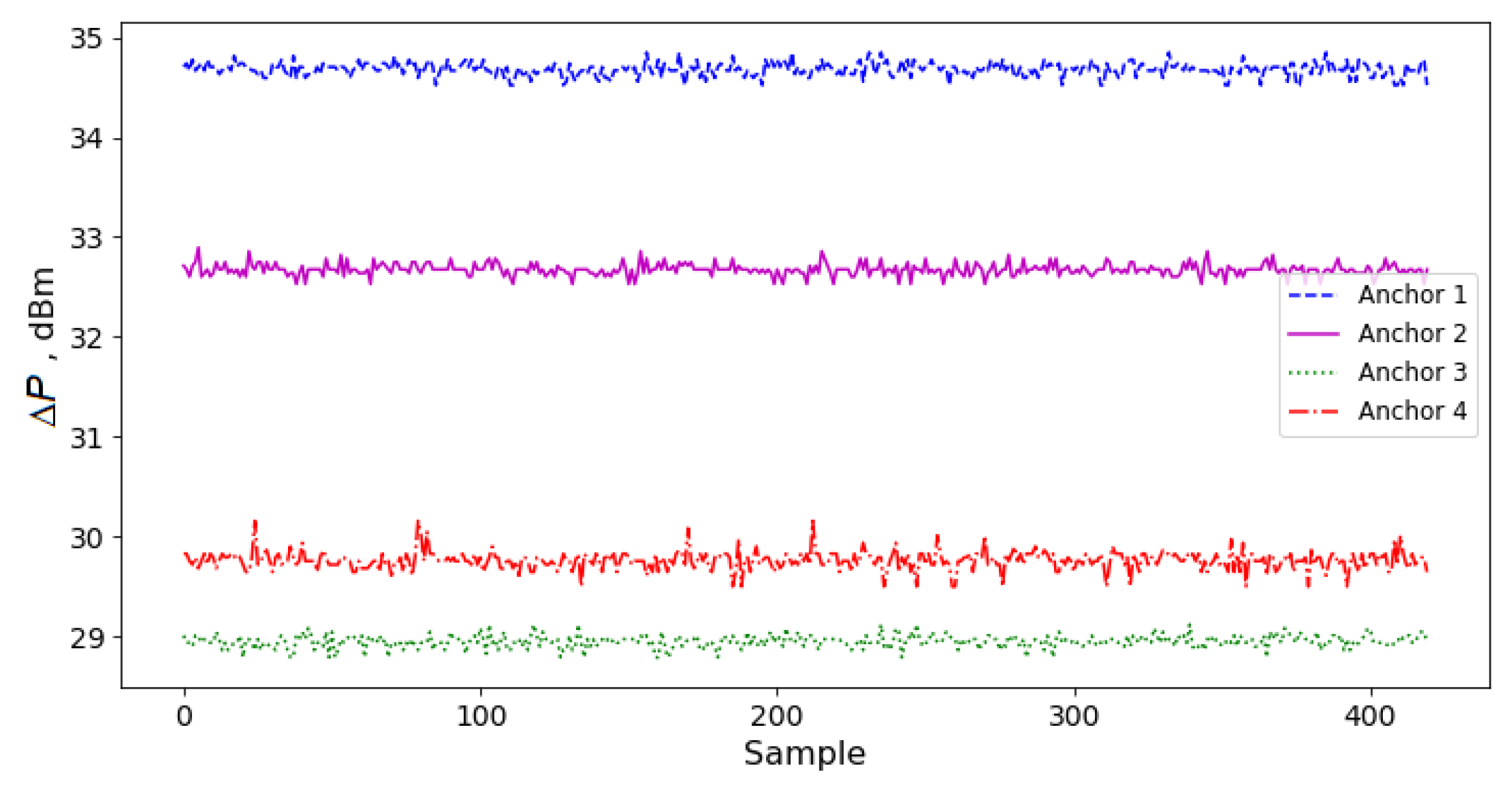
2.5. Wireless Signal Strength Measurement in Stationary Conditions

Two types of experimental measurements were carried out.

The aim of the first experiment was to determine the relationship between the actual power of the chaotic radio pulses at the receiver input and their power estimate obtained by the proposed method (Section 2.2). The actual received signal power was measured with an oscilloscope.

An experimental layout was assembled (Figure 5) with a stationary transmitter (target) and a receiver (anchor) ($T_X$ and $R_X$) at a distance of 1 m. A tunable attenuator, connected to the output of the transmitting module, added attenuation $Q_i$ to the emitted signal. The receiving module was connected to a digital storage oscilloscope and to a personal computer (PC).

The transmitting device ($T_X$) generates a sequence of chaotic radio pulses $s\left(t\right)$ of duration $t_P=0.625$ μs, repetition period $2t_P$, and average emission power in pulsed mode $P_P=9.5$ dBm. The transmitter signal is fed through a cable to the attenuator input that adds attenuation $Q_i$; then, the attenuated signal $s_Q\left(t\right)$ passes through the transmitting and receiving antennas, after which it is fed to the input of the receiving device ($R_X$). At the receiver output, the envelope $e\left(t\right)$ of signal $s_Q\left(t\right)$ is formed. A storage oscilloscope with a sampling rate of $f_S=2.5$ GHz stores the waveform of the envelope signal $e\left(t\right)$ in order to analyze the distributions of the instantaneous values of the amplitudes A. A comparison of these distributions with the estimates of the amplitude $A^{\ast }$ of radio pulses obtained with the proposed method allows us to verify the correctness of this method.

The measurements were carried out for the attenuation range: $Q_i$ = 0–46 dB with a step of 2 dB.

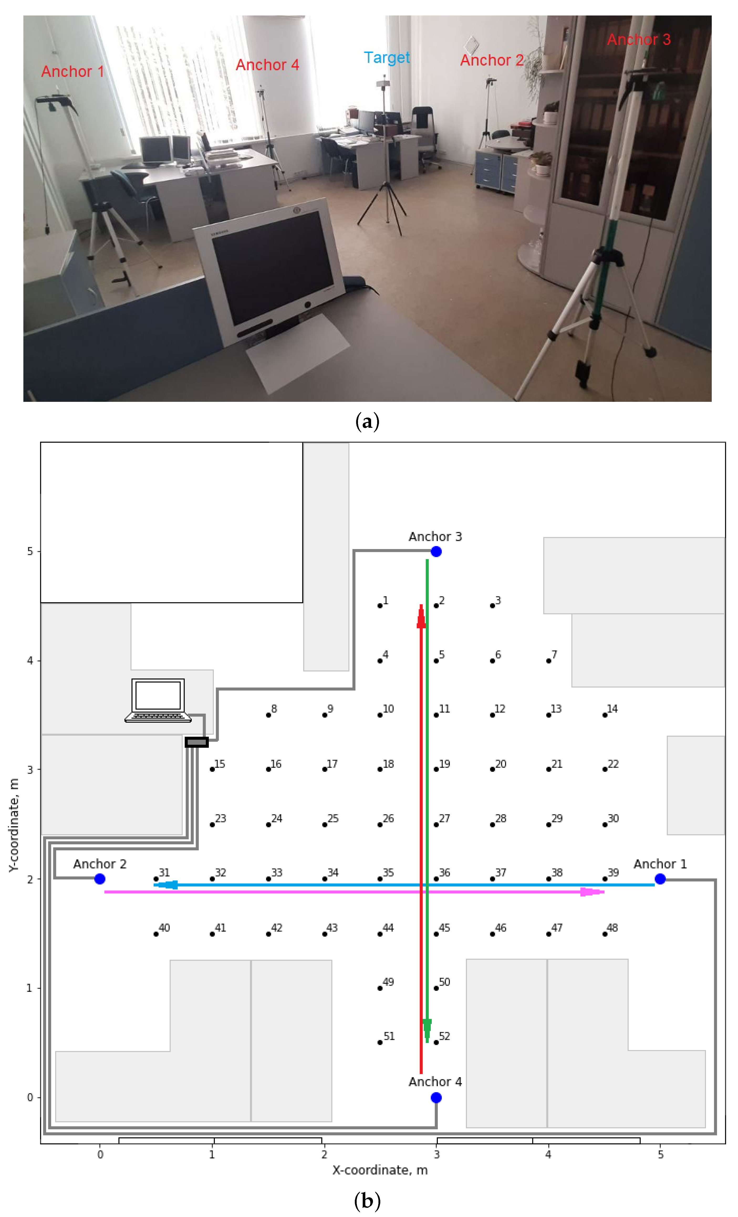
2.6. Schemes of Experimental Distance Measurement and Positioning

The second series of experiments is aimed at ranging and positioning using the proposed method of measuring signal power. Experiments on measuring distance between the emitter (target) and a receiver (anchor) (1D) and determining the position (2D) of the emitter (target) relative to several receivers (anchors) were carried out in an office space 6 × 6.5 m² (Figure 6a). Four receivers were located in pairs opposite each other at a distance of 5 m. The receivers were connected to the PC with USB cables. The emitter position was changed in accordance with the scheme shown in Figure 6b. We moved the emitter sequentially in each of the 52 positions of the grid (grid spacing 50 cm). The emitter and the receivers were placed at a height of 1.65 m above the floor.

The experiments were carried out in a real office room (not an anechoic chamber), which is characterized by multipath signal propagation. The emitter and the receivers were in direct visibility to each other (actually, for the receiver 3, points 15 and 23 were partially obscured by the furniture).

During the experiments, the transmitter constantly emitted a sequence of chaotic radio pulses. With a special program, the PC acquired data from the receivers (anchors 1–4) by polling them one by one. During a poll, the receiver forms a series of 100 $A^{\ast }$ estimates of the received signal amplitude. In total, for a given position of the emitter, a series of 400 polls (40,000 amplitude estimates $A^{\ast }$) is acquired from each of the receivers. Then, the emitter is moved to the next position and the measurement procedure is repeated.

The logic of measuring the distance assumes a preliminary determination of the path loss exponent n and the reference value of the received signal power $P_0$ at a distance $d_0$ in order to calculate expression (5). In this work, the accumulated measurement results were divided into two parts. The first part (10,000 measurements) was used to determine the path loss exponent n and reference values of the threshold at a distance $d_0$. The second part (30,000 measurements for each point 1–52) was used to study the accuracy of ranging and positioning.

Each concrete room is characterized by some average path loss exponent n, but as practice shows, the actual value of the path loss exponent can strongly depend on the geometry of the room and on the relative positions of the emitter and receiver. Therefore, in this paper, the value of the path loss exponent n was determined individually for each receiver. The exponent n was estimated by measuring the difference of the signal powers $P_1$ and $P_2$ (or the corresponding integer values $T_1$ and $T_2$ of the comparator) at two points spaced at a distance of $d_1$ and $d_2$ according to the expression:

$$n=\frac{(P_1-P_2)}{10\ast log\left(\frac{d_2}{d_1}\right)}=\frac{p(T_1-T_2)}{10\ast log\left(\frac{d_2}{d_1}\right)}$$

(10)

For receiver 1 (anchor 1), the values of $d_1$, $T_1$ and $d_2$, $T_2$ were determined at points (39, 31), for receiver 2 (anchor 2), they were determined at (31, 39), for receiver 3 (anchor 3), were determined at (3, 52), and for receiver 4 (anchor 4), they were determined at (52, 2). $T_1$ and $T_2$ were obtained by averaging over 10,000 measurements at each point. In all four cases, the difference $d_1-d_2=4$ m, which corresponded in order of magnitude to the dimensions of the room and thus allowed us to obtain the value of the path loss exponents characteristic of the room as a whole.

The experimental data served both to assess the accuracy of measuring the distance (positioning) on the line (1D) and on the plane (2D). To determine the distance on the line, we used the data obtained at the points located on the lines connecting pairs of receivers (Figure 6), namely: for receivers 1 and 2, measurements at points (31, 32, 33, 34, 35, 36, 37, 38, and 39), and for receivers 3 and 4, measurements at points (2, 5, 11, 19, 27, 36, 45, 50, and 52).

The distance measurement error in the course of the experiments was determined as the difference of the actual distance value d and its estimate $d^{\ast }$:

$$ϵ\left(d\right)=d-d^{\ast }$$

(11)

and the relative error was determined as the ratio of the distance measurement error to the actual distance:

$$ϵ{}_r\left(d\right)=ϵ\left(d\right)/d$$

(12)

When studying the positioning of the emitter on the plane (2D), we assigned point 36 as the reference point and estimated the distance relative to it using expression (5). For this point, we determined the reference power value and estimated the changes in the signal power (when moving over the plane) relative to this value. As a result, we obtained a set of estimates of the distance $d_i^{\ast }$ from the emitter to each of the receivers.

To calculate the emitter coordinates from the obtained distance estimates, we chose a min–max localization method [64,65] due to its simplicity, high speed and good results that had been obtained in previous works [64,65]. In this one-step method, from the estimates of the distances between the emitter and the receivers, the emitter coordinates on the plane were estimated using the following expressions:

$$\begin{array}{c}{x}_{min}={\displaystyle \underset{\begin{array}{c}0\le i\le N\end{array}}{max}}(x_i-d_i^{\ast })\\ x_{max}={\displaystyle \underset{\begin{array}{c}0\le i\le N\end{array}}{min}}(x_i+d_i^{\ast })\\ y_{min}={\displaystyle \underset{\begin{array}{c}0\le i\le N\end{array}}{max}}(y_i-d_i^{\ast })\\ y_{max}={\displaystyle \underset{\begin{array}{c}0\le i\le N\end{array}}{min}}(y_i+d_i^{\ast })\\ x^{\ast }=\frac{x_{min}+x_{max}}{2}\\ y^{\ast }=\frac{y_{min}+y_{max}}{2}\end{array}$$

(13)

where $x_i$ and $y_i$ are the coordinates of the ith receiver, $d_i^{\ast }$ is an estimate of the distance between the ith receiver and the emitter, N is the number of the receivers, and $x^{\ast }$, $y^{\ast }$ is the resulting estimate of the emitter coordinates.

3. Results

Experimental studies were carried out in accordance with the techniques described above.

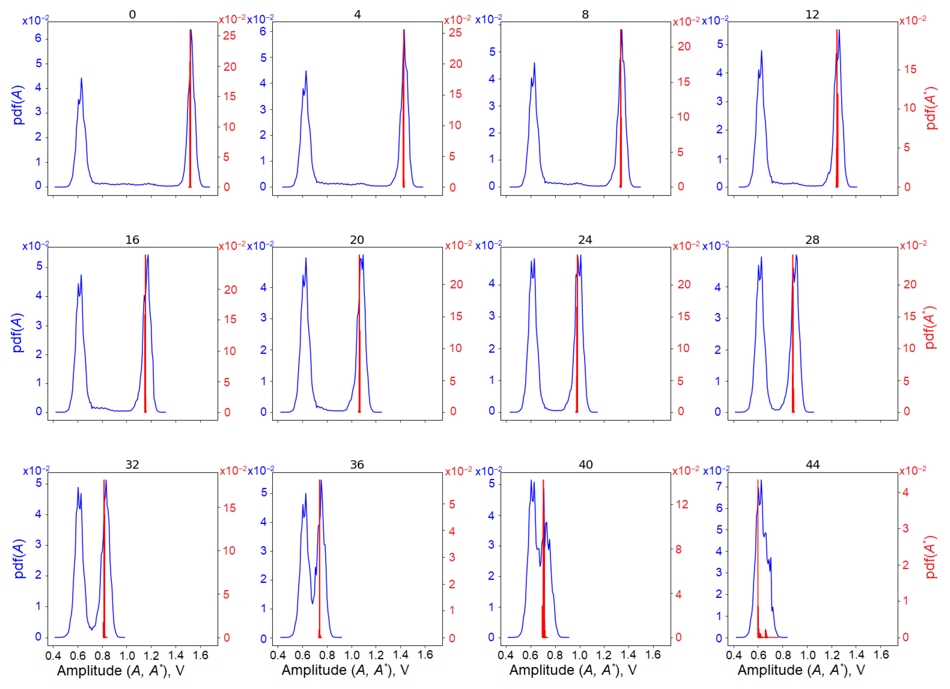
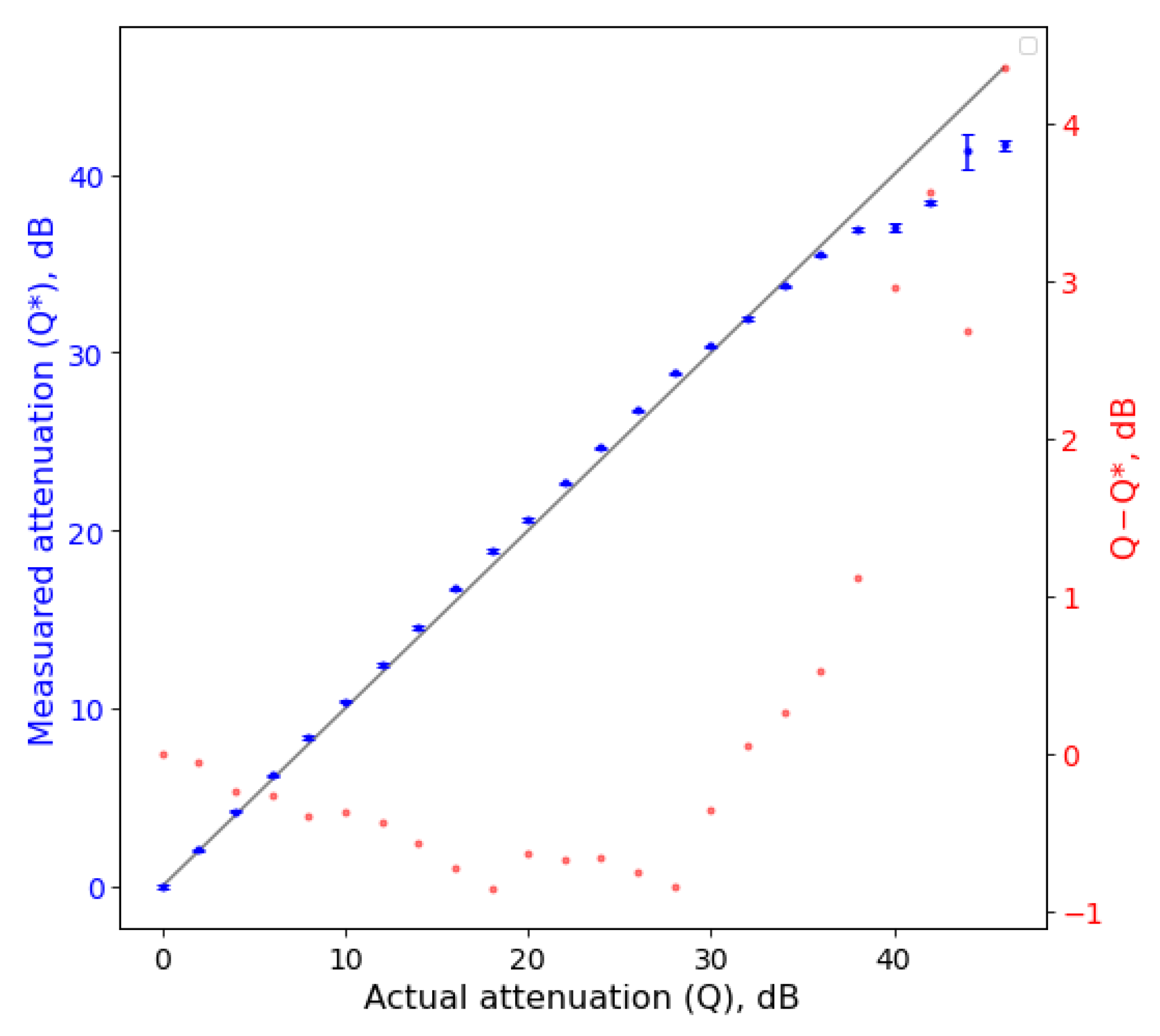
3.1. Measurement of Attenuation of the UWB Chaotic Signal under Stationary Conditions

At first, we carried out the experiments to confirm the correctness of measuring the power of chaotic signal by the proposed method by estimating the signal amplitude (Section 2.2). The measurements were made under stationary conditions for a distance of 1 m between the emitter and the receiver according to the scheme in Figure 5.

The measurement results are given in Figure 7, which shows the distribution densities $pdf\left(e\right(t\left)\right)$ of the instantaneous values of the amplitudes of the radio pulse envelope $e\left(t\right)$ obtained with a storage oscilloscope. Also shown are the distribution density functions $pdf\left(A^{\ast }\right)$ of the amplitude estimates $A^{\ast }$, which were obtained for different attenuation values $Q_i$ with the method proposed in this paper. The presented distribution densities $pdf\left(e\right(t\left)\right)$ are bimodal with two pronounced peaks. The left one corresponds to the instantaneous amplitudes concentrated around the signal level at the log detector output in the absence of radio pulses. The right one corresponds to the signal amplitudes in the presence of the chaotic radio pulse. As the signal attenuation increases, the average power of the radio pulse decreases and the corresponding peak of the distribution moves toward the peak corresponding to a no-pulse case. A characteristic feature of these distributions is that the width and shape of each of the peaks are preserved with increasing attenuation. At a value of $Q_i\ge 40$ dB, the peaks merge, which means that it becomes impossible to determine the presence or the absence of the radio pulse. Speaking of the positioning, this means an area of low signal-to-noise ratio (SNR) in which it is impossible to have acceptable distance accuracy.

Red color in Figure 7 denotes the distribution density of the amplitude estimates $A^{\ast }$ ($pdf\left(A^{\ast }\right)$). The peak of this function coincides with the right peak of $pdf\left(e\right(t\left)\right)$ that corresponds to the presence of radio pulses. This means that the amplitude estimate $A^{\ast }$ with a high accuracy corresponds to the real average amplitude of the radio pulse envelope, so it can be used to estimate the received signal power.

This fact is directly confirmed by the comparison of the received signal attenuation $Q_i^{\ast }$ measured by this method with the actual signal attenuation $Q_i$, as shown in Figure 8. The relation between the measured and actual attenuation values is well approximated by a straight line for $Q_i<38$ dB. For $Q_i>38$ dB, the error in determining the power is about 3 dB, as is expected from the distribution of instantaneous values.

Using the dependence of the measured power on the attenuation in the channel, we can estimate the power budget of the channel in free space approximation, since the attenuator here stands for the path loss which would have been added to the signal with a real increase in the distance between the emitter and the receiver in free space. According to Figure 8, the maximum power measurement error (that is still below 1 dB) is observed at an attenuation of $Q_r$ = 38 dB. The path loss for a signal of frequency $f_0$ at a distance d from the emission source is described by the expression [66]

$$Q_d=10lo{g}_{10}\left[{\left(\frac{4\pi d{f}_0}{c}\right)}^2\right],$$

where $f_0=\sqrt{f_1{f}_2}$ is the geometric mean of the UWB signal frequency [67]. Substituting $f_1\simeq 3$ GHz and $f_2\simeq 5$ GHz into this expression, we find that the signal attenuation (path loss) at a distance of d = 1 m is $L_{1m}$ = 44.2 dB. With the emitted signal power per pulse $P_{Tx}$ = 12.5 dBm, the receiver sensitivity [62] $S=-70$ dBm, and $LNA$ gain $G_{LNA}=15$ dB, we have:

$$M=P_{Tx}-L_{1m}-S+G_{LNA}-Q_r$$

(14)

substituting the appropriate values into (14), we obtain $M=14.7$ dBm, which is the power reserve of the received signal that is necessary to measure power with an accuracy of 1 dBm.

Consequently, using expression (5), we obtain the maximum theoretical distance (in free space with n = 2) at which the distance can be measured; it is approx. 80 m (79.4 m). This experiment also confirms that the proposed method can give a practically acceptable distance measurement accuracy.

3.2. Distance Measurement in 1D

In agreement with the algorithm described above (Section 2.3), first we present the results of measuring the distance between the emitter (target) and each of the receivers (anchors) (1D), and then we present the results of 2D positioning on the plane.

One of the main problems that limit the accuracy of wireless ranging is random fluctuation of the RSS over time. In order to analyze the stability of the RSS measured with the proposed method, we calculated the standard deviation of the RSS values from the mean value for all 4 receivers and 52 emitter locations. At each point, measurements were carried out within 90 s. The maximum std value for all measurements was 0.24 dBm, and the spread (the difference between the maximum and minimum values) was 1.87 dBm. As an illustration, Figure 9 shows the results of measuring the strength of the signal received by each of the anchors for 1 s when the emitter is located at one of the points (here, point 4). As can be seen in the figure, the obtained RSS values have low variability (<0.5 dBm). The obtained data reflect the instrumental error of the equipment and of the method used in a stationary situation in an office building in the presence of external interference and technical noise, but they do not take into account the whole variety of possible sources of RSS fluctuations, such as the presence of people, the arrangement of furniture, movement of the emission source or other technical devices, random electric surges, etc.

The results obtained in 1D mode are given in Figure 10, which shows the measured distance as a function of the actual distance between the emitter and the receiver.

Note that the dependencies of the measured RSS and the measured distance on the actual distance are relatively smooth and predictable. In the region of short distances, where the SNR is high, and the propagation effects are insignificant, there are no unpredictable fluctuations of the measured values caused by RSS fluctuations. With a further increase in the distance, the effects of multipath signal propagation appear, which reduce the capabilities of the measurement method. A distance measurement accuracy of no worse than 20 cm is observed in the area of up to 2.5 m between the emitter and receiver.

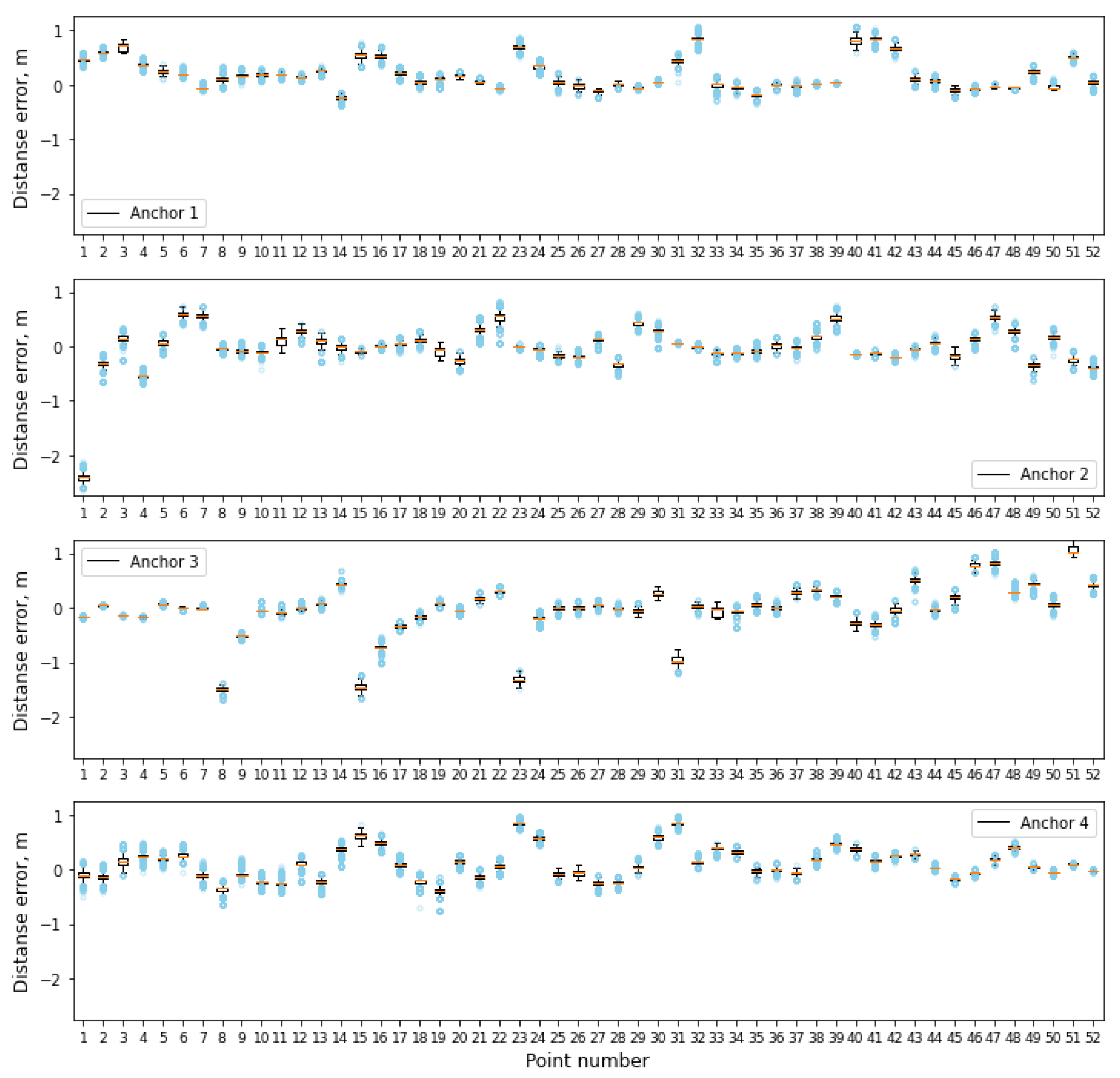
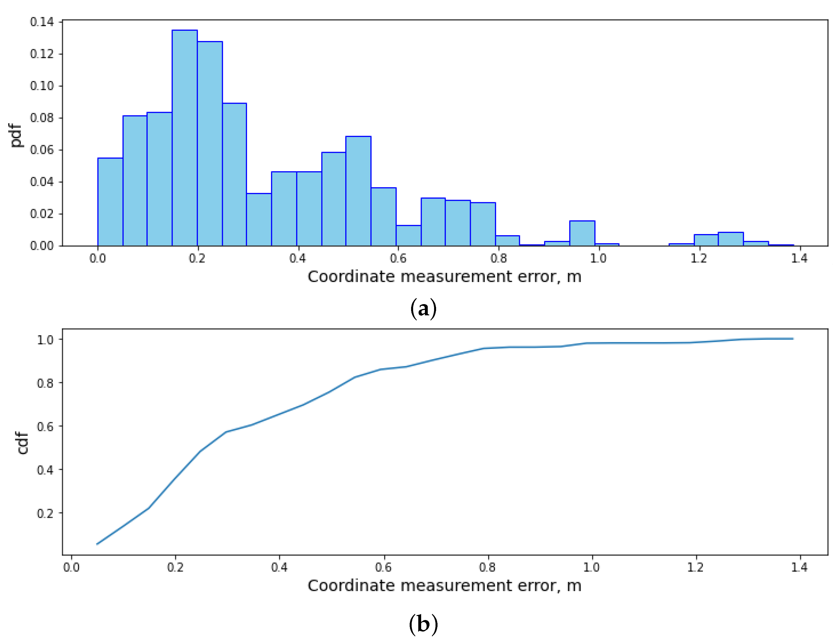
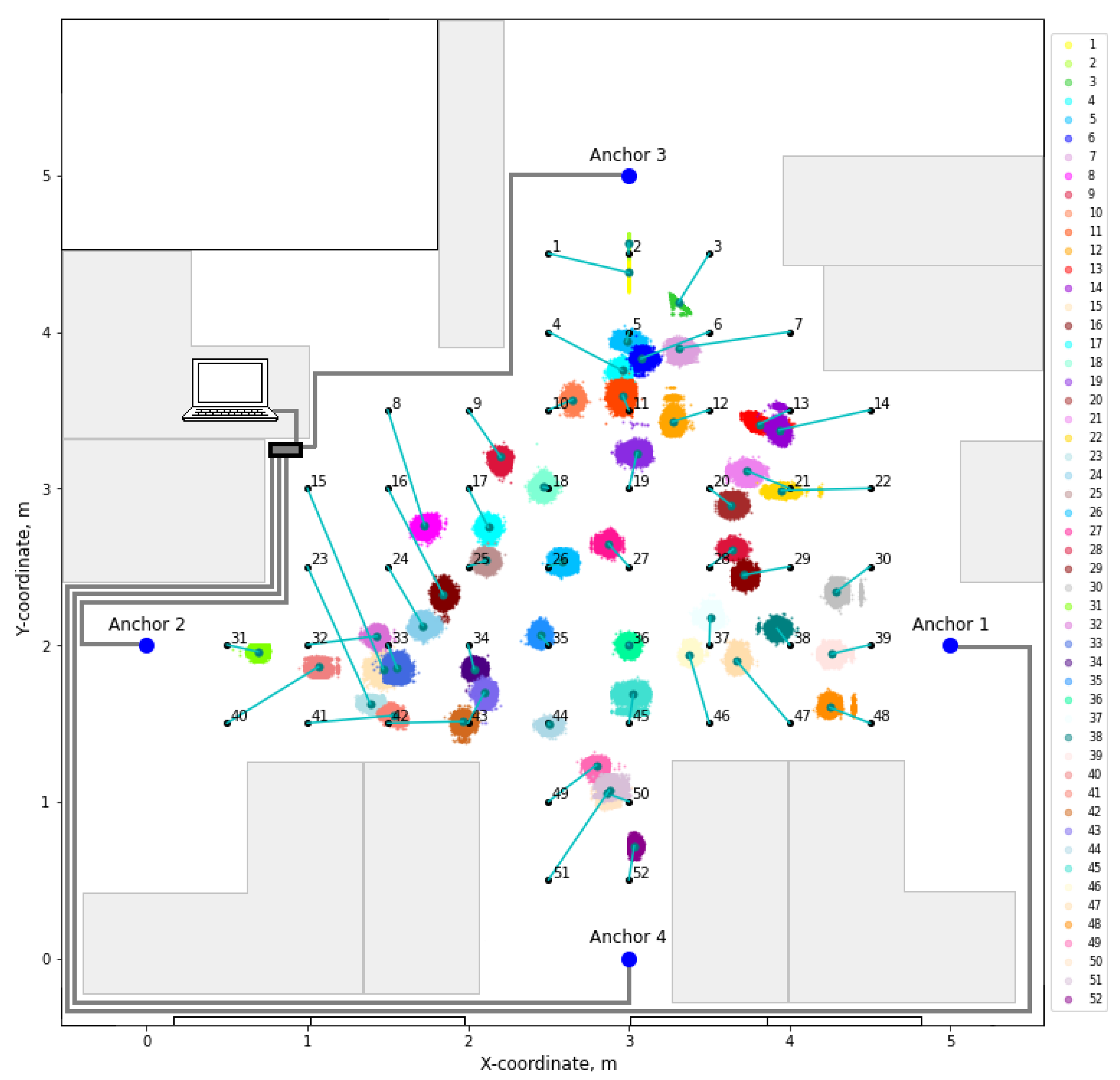
3.3. Two-Dimensional (2D) Positioning Experiment

Figure 11 shows the results of determining the distance measurement error (11) for all 52 emitter (target) positions relative to each of the four receivers (anchors). The position number is indicated along the horizontal axis, and the distance measurement error is indicated along the vertical axis.

This dependence has a characteristic jump-like form, because the absolute error is minimal when the emitter is near the receiver and reaches its maximum when the emitter is moved away from the receiver. For the vast majority of positions, the absolute median value of the distance measurement error does not exceed 1 m for all receivers. An absolute error above 1.5 m is observed for point 1 relative to receiver 2 and points 8, 15 relative to receiver 3. This is because the path between these point locations and the corresponding receivers is partially obscured by the furniture and does not fully correspond to LOS conditions. Note also that for all measurements, the variance of the deviation from the median measured value is small and does not exceed 10 cm with no significant outliers. Although the actual median value of the measured distance may deviate from the true value by more than 10 cm, the deviation variance indicates the stability of the measurements. Therefore, in the future, we can raise the question of developing methods for mitigating these deviations.

Based on the measured distances, for each of the emitter positions, the coordinates of the emitter on the plane were determined using the min–max localization method (13). The positioning error or coordinate measurement error ($cme$), i.e., the deviation of the measured coordinate from the real one in the $R^2$ norm is calculated as

$$cme=\sqrt{{(x-x^{\ast })}^2+{(y-y^{\ast })}^2}$$

(15)

where x, y are the actual position coordinates, and $x^{\ast }$, $y^{\ast }$ are the estimates of the position coordinates.

Table 1. Ranging and positioning errors.

	MAE	MedAE	STD	RMSE	90% of AE Is Less Than
Ranging error, m	0.25	0.16	0.30	0.39	0.59
Relative ranging error	0.09	0.07	0.09	0.13	0.22
Positioning error, m	0.34	0.26	0.25	0.42	0.69

shows the mean absolute values, median absolute values, standard deviation, RMSEs and upper boundary of the interval into which fall 90% of the absolute ranging errors (AE), relative ranging errors and 2D positioning errors averaged over all 52 emitter positions and 4 receivers.

In order to obtain an idea of the distribution of the positioning errors, the distribution densities (Figure 12a) and cumulative probability distribution functions were calculated (Figure 12b) for the deviations of the measured coordinate from the actual one.

In the figure, these data are given for measurements collected from all 52 positions. For the vast majority of points (with the exception of points 15 and 23), the error in determining coordinates does not exceed 0.8 m for 100% of the measurements. For 90% of the measurements, the error does not exceed 0.69 m (see Table 1). For convenience, in Figure 13, we show the actual positions of the emitter and indicate them by numbers, as in Figure 6b. The obtained coordinate estimates are shown with colored dots. Turquoise lines connect the actual and the average measured position of the emitter. Note that the measured coordinates are clustered together for each position, which will facilitate the design of the methods for correcting the emitter coordinates in the future.

As can be seen in the figure, in the center of the room, the positioning accuracy is high, but in areas remote from the receivers, it decreases. This effect can be caused by a number of factors, such as a systematic error of the method, the growth of additive interference with increasing distance, proximity to walls and furniture, causing multiple reflections and distorting the received signal, the phenomenon of multipath amplification [68] characteristic for chaotic signals as a result of adding the powers of signals arriving along different propagation paths, etc.

To verify the reproducibility of the results, as well as to investigate the effect of antenna orientation, we carried out a second series of experiments. In these experiments, for each of the 52 emitter locations, data were accumulated for two antenna orientations:

1. The antenna plane is parallel to the XZ plane (Figure 6);

2. The antenna plane is parallel to the YZ plane.

Studies with antenna orientation in the XY plane were omitted, since this research only considers positioning on a plane, and the use of an emitter with an antenna oriented in the XY plane was not in the scenario.

For the received signal power at the reference point (point 36), we took the arithmetic mean of the values for two antenna orientations for further distance calculations using expression (5). As for the attenuation exponent n of each anchor (Anchor 1–4), we took the values obtained during the first series of experiments ($n_1$ = 1.68, $n_2$ = 1.78, $n_3$ = 1.90, $n_4$ = 1.64), assuming that the signal propagation conditions in the room did not change significantly. The results of the second series of experiments are shown in

Table 2. Ranging and positioning errors for different antenna orientations.

	MAE	MedAE	STD	RMSE	90% of AE Is Less Than
Antenna in XZ plane
Ranging error, m	0.29	0.21	0.27	0.39	0.59
Relative ranging error	0.11	0.09	0.09	0.15	0.24
Positioning error, m	0.34	0.26	0.26	0.42	0.63
Antenna in YZ plane
Ranging error, m	0.32	0.24	0.29	0.43	0.66
Relative ranging error	0.13	0.10	0.11	0.16	0.25
Positioning error, m	0.37	0.33	0.27	0.46	0.70

. The table shows the mean absolute error (MAE), the median absolute error (MedAE), the standard deviation of the absolute error (STD), the root mean square error (RMSE), and the upper limit of the interval into which fall 90% of the absolute errors (AEs) of the distance measurement, relative distance measurement and 2D positioning errors for all 52 emitter positions, 4 receivers, and 2 antenna orientation options.

From the data presented in Table 1 and Table 2, it is clear that the results are reproduced from experiment to experiment with fairly good accuracy, and that the change in the antenna orientation does not lead to a dramatic change in the positioning accuracy. It should be noted that in this work, we deliberately did not use any post-processing methods to the obtained power measurement results. The errors are clearly regular and have low variance, which creates prerequisites for further improvements of the positioning accuracy by various signal post-processing methods, choosing an appropriate positioning method and the use of such approaches as fingerprinting.

4. Discussion

Methods for determining the object coordinates in wireless networks are being constantly discussed in the literature. Practice shows that for nondirectional systems, it is advisable to use RF positioning methods. Among these methods, power measurement is technically one of the most accessible, so the power measurement-based localization methods are very popular.

On the one hand, the positioning systems based on the time of arrival or angle of arrival show better performance compared to the positioning based on RSS measurements. On the other hand, from a technical point of view, the time or angle measurement is a much more complicated problem that requires the development of technical means that must be built into the transceivers. However, the RSS measurement can be part of the data transmission process both in narrowband and in UWB communication systems.

The variety of technologies and methods for wireless measurements is extremely large. The experimental studies described in the literature are highly heterogeneous both in the approaches used and in the scenarios of the experiments performed. Therefore, it is difficult to compare them with each other. For comparison, we have chosen several works, the experimental conditions of which are close to the conditions described in this work, and their results can be compared. The selection criteria included the small size of the office or laboratory-type premises, the use of an RSS and the path loss model to approximate distance between nodes.

Table 3. Comparison of different technologies under similar experimental conditions.

Ref.	Technology	Room Size	Distance b/w	MAE	90% of AE
			the Anchors, m		Is Less Than
[69]	WiFi	10.8 m × 7.3 m	1–5	0.843
		5.6 m × 5.9 m	1–5	0.486
[69]	BLE	10.8 m × 7.3 m	1–5	0.661
		5.6 m × 5.9 m	1–5	0.844
[69]	ZigBee	10.8 m × 7.3 m	1–5	0.882
		5.6 m × 5.9 m	1–5	0.911
[69]	LoRaWAN	10.8 m × 7.3 m	1–5	0.846
		5.6 m × 5.9 m	1–5	1.534
[65]	CC2500 RF	3.6 m × 6.2 m		1.04–1.52
		(test area)
		4.0 m × 2.8 m		0.53
		(test area)
[37]	UWB USP		3–10		1.5
This	UWB Chaotic	6 m × 6.5 m
work	Radio	5 m × 5 m	5	0.34–0.37	0.7
	Pulses	(test area)

summarizes the results from several studies: Ref. [69] which compares Wi-Fi, BLE, ZigBee and LoRaWAN technologies; Ref. [65] which examines a system on the CC2500 RF chip; Ref. [37] dedicated to positioning based on UWB USP; and the present work. All the papers present results for comparable room types and sizes, comparable test bench sizes, and LOS conditions. Scenarios that involve the presence and movement of people, which is a factor that causes significant signal fluctuations, are not considered.

As we can see, having comparable parameters, the proposed method is at least no worse, and in some cases, it exceeds the characteristics of mass wireless systems in terms of positioning accuracy. The significance of the type of the signals used in this work (ultra-wideband chaotic) is the immunity to multipath fading in multipath environments, whereas the signal accumulation allows us to tune out the signal power variations within the UWB chaotic radio pulse.

This work was necessary because the issue of measuring the power of UWB chaotic signals has not yet been discussed in the literature, and from theoretical considerations, it was clear that the positioning accuracy achieved by measuring power would be higher for such signals than for narrowband signals subject to multipath fading. A low dispersion and a high measurement speed allow us to either reduce the dispersion by averaging, or organize multiple access with an acceptable update rate, thus sacrificing dispersion. The proposed method can be implemented on wireless devices that form a wireless sensor network.

The solution to the task of determining signal strength can be useful for a wider range of applications than just emitter localization. The advantage of the proposed method is that the update rate of power measurement is very high: only about a hundred chaotic radio pulses are necessary to determine the signal power. With a pulse duration of the order of a microsecond, one measurement is several hundred microseconds, so the method allows thousands of power measurements per second. One can make instant measurements of the power distribution of the signals emitted by UWB sources in the room. Using this distribution, one can simultaneously position objects (well-known fingerprinting applied to UWB chaotic signals) and monitor the indoor situation. The distribution of received power is very sensitive to changes in the situation, and the proposed method is one of the practical tools of tracking it.

To date, there is no single picture or established practice from which one could draw a conclusion about the advisability of using UWB chaotic signals to solve positioning problems. The reason for this is the lack of explicit practically effective solutions that would show the superiority of such systems over narrowband mass-purpose systems, for which there are ready-made hardware solutions and for which developers can, using available powerful computing resources of modern smartphones, work out various methods for improving the positioning, and through smartphones, these methods can be built into the existing wireless digital infrastructure. In this work, we tried to take a step in this direction and to show that systems based on UWB chaotic oscillations can demonstrate good performance using fundamentally simple technical solutions.

5. Conclusions and Future Work

The manuscript presents results of an experimental study of ranging and positioning based on measuring the power of UWB chaotic radio pulses. The difficulties of creating indoor positioning methods based on signal strength measurements are well known: a strong dependence on signal propagation conditions and uncertainties associated with external interference falling into the signal band, which limit the accuracy of ranging and positioning based on measured distances. In this regard, this study of the positioning problem using a little-studied type of UWB signals—chaotic radio pulses—seems relevant and in demand.

As a result of this study, we obtained the following:

• A new method for measuring the power of UWB chaotic radio pulses transmitted through a wireless communication channel.
• The proposed method for measuring the power of chaotic radio pulses can be integrated into the data transmission process of communication systems based on chaotic radio pulses, since it essentially uses the same signal processing.
• The system is shown to provide stable power measurements under stationary conditions with a standard deviation of 0.24 dBm.
• For the first time, experimental studies have been carried out on the indoor positioning of objects in 2D based on measurements of the power of UWB chaotic radio pulses.
• In a real indoor wireless communication channel, the proposed scheme and its experimental implementation provide an accuracy of $34$ cm, which is better than the accuracy of other mass-purpose wireless systems (using signal power measurements) under comparable conditions.
• The presented results can be used as a baseline for further development and research of the positioning methods based on UWB chaotic signals.

The questions of increasing the measurement accuracy by choosing signal post-processing methods, choosing a localization method, compensation of the effects of multipath propagation and interference from other radio systems, or people moving in the room, are beyond the scope of this work and will be the subject of future research.

References

1. Sesyuk, A.; Ioannou, S.; Raspopoulos, M. A Survey of 3D Indoor Localization Systems and Technologies. Sensors 2022, 22, 9380. [Google Scholar] [CrossRef]
2. Hayward, S.; van Lopik, K.; Hinde, C.; West, A. A Survey of Indoor Location Technologies, Techniques and Applications in Industry. Internet Things 2022, 20, 100608. [Google Scholar] [CrossRef]
3. Bourdoux, A.; Barreto, A.N.; van Liempd, B.; de Lima, C.; Dardari, D.; Belot, D.; Lohan, E.S.; Seco-Granados, G.; Sarieddeen, H.; Wymeersch, H.; et al. 6G White Paper on Localization and Sensing. arXiv 2020, arXiv:eess.SY/2006.01779. [Google Scholar] [CrossRef]
4. Senevirathna, N.M.; De Silva, O.; Mann, G.K.I.; Gosine, R.G. Asymptotic Gradient Clock Synchronization in Wireless Sensor Networks for UWB Localization. IEEE Sens. J. 2022, 22, 24578–24592. [Google Scholar] [CrossRef]
5. Yang, T.; Cabani, A.; Chafouk, H. A Survey of Recent Indoor Localization Scenarios and Methodologies. Sensors 2021, 21, 8086. [Google Scholar] [CrossRef]
6. Nessa, A.; Adhikari, B.; Hussain, F.; Fernando, X.N. A Survey of Machine Learning for Indoor Positioning. IEEE Access 2020, 8, 214945–214965. [Google Scholar] [CrossRef]
7. Karakusak, M.Z.; Kivrak, H.; Ates, H.F.; Ozdemir, M.K. RSS-Based Wireless LAN Indoor Localization and Tracking Using Deep Architectures. Big Data Cogn. Comput. 2022, 6, 84. [Google Scholar] [CrossRef]
8. Nabati, M.; Ghorashi, S.A. A real-time fingerprint-based indoor positioning using deep learning and preceding states. Expert Syst. Appl. 2023, 213, 118889. [Google Scholar] [CrossRef]
9. Wang, L.; Shang, S.; Wu, Z. Research on Indoor 3D Positioning Algorithm Based on WiFi Fingerprint. Sensors 2023, 23, 153. [Google Scholar] [CrossRef]
10. Guo, X.; Ansari, N.; Hu, F.; Shao, Y.; Elikplim, N.R.; Li, L. A Survey on Fusion-Based Indoor Positioning. IEEE Commun. Surv. Tutor. 2020, 22, 566–594. [Google Scholar] [CrossRef]
11. Farahsari, P.S.; Farahzadi, A.; Rezazadeh, J.; Bagheri, A. A Survey on Indoor Positioning Systems for IoT-Based Applications. IEEE Internet Things J. 2022, 9, 7680–7699. [Google Scholar] [CrossRef]
12. Savić, T.; Vilajosana, X.; Watteyne, T. Constrained Localization: A Survey. IEEE Access 2022, 10, 49297–49321. [Google Scholar] [CrossRef]
13. Niemelä, V.; Haapola, J.; Hämäläinen, M.; Iinatti, J. An Ultra Wideband Survey: Global Regulations and Impulse Radio Research Based on Standards. IEEE Commun. Surv. Tutor. 2017, 19, 874–890. [Google Scholar] [CrossRef]
14. Breed, G. A Summary of FCC Rules for Ultra Wideband Communications. High Freq. Electron. 2005, 4, 42–44. [Google Scholar]
15. Mandke, K.; Nam, H.; Zuniga, C.; Rappaport, T. The Evolution of Ultra Wide Band Radio for Wireless Personal Area Networks. High Freq. Electron. 2003, 2, 22–32. [Google Scholar]
16. IEEE 802.15 WPAN High Rate Alternative PHY Task Group 3a (TG3a). Available online: https://www.ieee802.org/15/pub/TG3a_old.html (accessed on 24 October 2023).
17. IEEE Std 802.15.4a-2007 (Amendment to IEEE Std 802.15.4-2006); IEEE Standard for Information Technology—Local and Metropolitan Area Networks– Specific Requirements– Part 15.4: Wireless Medium Access Control (MAC) and Physical Layer (PHY) Specifications for Low-Rate Wireless Personal Area Networks (WPANs): Amendment 1: Add Alternate PHYs. IEEE: New York City, NY, USA, 2007; pp. 1–210. [CrossRef]
18. 802.15.6-2012; IEEE Standard for Local and Metropolitan Area Networks—Part 15.6: Wire-Less Body Area Networks. IEEE: New York City, NY, USA, 2012; pp. 1–271.
19. 802.15.4z-2020; IEEE Standard for Low-Rate Wireless Networks–Amendment 1: Enhanced Ultra Wideband (UWB) Physical Layers (PHYs) and Associated Ranging Techniques. IEEE Press: New York City, NY, USA, 2020; Amendment to IEEE Std 802.15.4-2020. pp. 1–174.
20. Stocker, M.; Brunner, H.; Schuh, M.; Boano, C.A.; Römer, K. On the Performance of IEEE 802.15.4z-Compliant Ultra-Wideband Devices. In Proceedings of the 2022 Workshop on Benchmarking Cyber-Physical Systems and Internet of Things (CPS-IoTBench), Milan, Italy, 3–6 May 2022; pp. 28–33. [Google Scholar] [CrossRef]
21. Chen, H.; Chen, Z.; Ou, R.; Chen, R.; Wu, Z.; Li, B. A 4-to-9GHz IEEE 802.15.4z-Compliant UWB Digital Transmitter with Reconfigurable Pulse-Shaping in 28nm CMOS. In Proceedings of the 2022 IEEE Radio Frequency Integrated Circuits Symposium (RFIC), Denver, CO, USA, 19–21 June 2022; pp. 99–102. [Google Scholar] [CrossRef]
22. Agiwal, M.; Roy, A.; Saxena, N. Next Generation 5G Wireless Networks: A Comprehensive Survey. IEEE Commun. Surv. Tutor. 2016, 18, 1617–1655. [Google Scholar] [CrossRef]
23. Alavi, B.; Pahlavan, K. Studying the effect of bandwidth on performance of uwb positioning systems. In Proceedings of the IEEE Wireless Communications and Networking Conference, WCNC 2006, Las Vegas, NV, USA, 3–6 April 2006; Volume 2, pp. 884–889. [Google Scholar] [CrossRef]
24. Bharadwaj, R.; Parini, C.; Alomainy, A. Analytical and Experimental Investigations on Ultrawideband Pulse Width and Shape Effect on the Accuracy of 3-D Localization. IEEE Antennas Wirel. Propag. Lett. 2016, 15, 1116–1119. [Google Scholar] [CrossRef]
25. Dabove, P.; Di Pietra, V.; Piras, M.; Jabbar, A.A.; Kazim, S.A. Indoor positioning using Ultra-wide band (UWB) technologies: Positioning accuracies and sensors’ performances. In Proceedings of the 2018 IEEE/ION Position, Location and Navigation Symposium (PLANS), Monterey, CA, USA, 23–26 April 2018; pp. 175–184. [Google Scholar] [CrossRef]
26. De Angelis, A.; Dwivedi, S.; Händel, P.; Moschitta, A.; Carbone, P. Ranging results using a UWB platform in an indoor environment. In Proceedings of the 2013 International Conference on Localization and GNSS (ICL-GNSS), Turin, Italy, 25–27 June 2013; pp. 1–5. [Google Scholar] [CrossRef]
27. Zhang, C.; Kuhn, M.J.; Merkl, B.C.; Fathy, A.E.; Mahfouz, M.R. Real-Time Noncoherent UWB Positioning Radar With Millimeter Range Accuracy: Theory and Experiment. IEEE Trans. Microw. Theory Tech. 2010, 58, 9–20. [Google Scholar] [CrossRef]
28. Sahinoglu, Z.; Gezici, S.; Güvenc, I. Ultra-Wideband Positioning Systems: Theoretical Limits, Ranging Algorithms, and Protocols; Cambridge University Press: Cambridge, UK, 2008. [Google Scholar] [CrossRef]
29. Alarifi, A.; Al-Salman, A.; Alsaleh, M.; Alnafessah, A.; Al-Hadhrami, S.; Al-Ammar, M.A.; Al-Khalifa, H.S. Ultra Wideband Indoor Positioning Technologies: Analysis and Recent Advances. Sensors 2016, 16, 707. [Google Scholar] [CrossRef]
30. Che, F.; Ahmed, Q.Z.; Lazaridis, P.I.; Sureephong, P.; Alade, T. Indoor Positioning System (IPS) Using Ultra-Wide Bandwidth (UWB)—For Industrial Internet of Things (IIoT). Sensors 2023, 23, 5710. [Google Scholar] [CrossRef]
31. Molisch, A.; Balakrishnan, K.; Cassioli, D.; Chong, C.; Emami, S.; Fort, A.; Karedal, J.; Kunish, J.; Schantz, H.; Siwiak, K. 802.15.4a Channel Model–Final Report. 2004, pp. 1–40. Available online: https://www.ieee802.org/15/pub/04/15-04-0662-02-004a-channel-model-final-report-r1.pdf (accessed on 24 October 2023).
32. Molisch, A.F. Ultra-Wide-Band Propagation Channels. Proc. IEEE 2009, 97, 353–371. [Google Scholar] [CrossRef]
33. Zanella, A. Best Practice in RSS Measurements and Ranging. IEEE Commun. Surv. Tutor. 2016, 18, 2662–2686. [Google Scholar] [CrossRef]
34. IEEE Std 802.15.4-2015; IEEE Standard for Low-Rate Wireless Networks. IEEE: New York City, NY, USA, 2016; Revision of IEEE Std 802.15.4-2011. pp. 1–709. [CrossRef]
35. Zhu, X.; Qu, W.; Qiu, T.; Zhao, L.; Atiquzzaman, M.; Wu, D.O. Indoor Intelligent Fingerprint-Based Localization: Principles, Approaches and Challenges. IEEE Commun. Surv. Tutor. 2020, 22, 2634–2657. [Google Scholar] [CrossRef]
36. Yaro, A.S.; Maly, F.; Prazak, P. A Survey of the Performance-Limiting Factors of a 2-Dimensional RSS Fingerprinting-Based Indoor Wireless Localization System. Sensors 2023, 23, 2545. [Google Scholar] [CrossRef]
37. Gigl, T.; Janssen, G.J.; Dizdarevic, V.; Witrisal, K.; Irahhauten, Z. Analysis of a UWB Indoor Positioning System Based on Received Signal Strength. In Proceedings of the 2007 4th Workshop on Positioning, Navigation and Communication, Hannover, Germany, 22 March 2007; pp. 97–101. [Google Scholar] [CrossRef]
38. Bellusci, G.; Janssen, G.J.M.; Yan, J.; Tiberius, C.C.J.M. Low complexity ultra-wideband ranging in indoor multipath environments. In Proceedings of the 2008 IEEE/ION Position, Location and Navigation Symposium, Monterey, CA, USA, 5–8 May 2008; pp. 394–401. [Google Scholar] [CrossRef]
39. Botler, L.; Diwold, K.; Roemer, K. Improving Signal-Strength-Based Distance Estimation in UWB Transceivers. In Proceedings of the Cyber-Physical Systems and Internet of Things Week 2023, San Antonio, TX, USA, 9–12 May 2023; CPS-IoT Week ’23. pp. 61–66. [Google Scholar] [CrossRef]
40. Sourya, A.; Dutta, S.; Chandra, A.; Prokes, A.; Kim, M. Find My Car: Simple RSS-based UWB Localization Algorithms for Single and Multiple Transmitters. In Proceedings of the 2020 IEEE Latin-American Conference on Communications (LATINCOM), Santo Domingo, Dominican Republic, 18–20 November 2020; pp. 1–6. [Google Scholar] [CrossRef]
41. Barbi, M.; Garcia-Pardo, C.; Nevárez, A.; Pons Beltrán, V.; Cardona, N. UWB RSS-Based Localization for Capsule Endoscopy Using a Multilayer Phantom and In Vivo Measurements. IEEE Trans. Antennas Propag. 2019, 67, 5035–5043. [Google Scholar] [CrossRef]
42. Wang, S.; Waadt, A.; Burnic, A.; Xu, D.; Kocks, C.; Bruck, G.H.; Jung, P. System implementation study on RSSI based positioning in UWB networks. In Proceedings of the 2010 7th International Symposium on Wireless Communication Systems, York, UK, 19–22 September 2010; pp. 36–40. [Google Scholar] [CrossRef]
43. Ivanov, S.; Kuptsov, V.; Badenko, V.; Fedotov, A. RSS/TDoA-Based Source Localization in Microwave UWB Sensors Networks Using Two Anchor Nodes. Sensors 2022, 22, 3018. [Google Scholar] [CrossRef] [PubMed]
44. Chong, A.M.S.; Yeo, B.C.; Lim, W.S. Integration of UWB RSS to Wi-Fi RSS fingerprinting-based indoor positioning system. Cogent Eng. 2022, 9, 2087364. [Google Scholar] [CrossRef]
45. Alonge, F.; Branciforte, M.; Motta, F. A Novel Method of Distance Measurement Based on Pulse Position Modulation and Synchronization of Chaotic Signals Using Ultrasonic Radar Systems. IEEE Trans. Instrum. Meas. 2009, 58, 318–329. [Google Scholar] [CrossRef]
46. Corron, N.J.; Stahl, M.T.; Chase Harrison, R.; Blakely, J.N. Acoustic detection and ranging using solvable chaos. Chaos Interdiscip. J. Nonlinear Sci. 2013, 23, 023119. [Google Scholar] [CrossRef]
47. Beal, A.N.; Cohen, S.D.; Syed, T.M. Generating and Detecting Solvable Chaos at Radio Frequencies with Consideration to Multi-User Ranging. Sensors 2020, 20, 774. [Google Scholar] [CrossRef]
48. Zhang, M.; Ji, Y.; Zhang, Y.; Wu, Y.; Xu, H.; Xu, W. Remote Radar Based on Chaos Generation and Radio Over Fiber. IEEE Photonics J. 2014, 6, 1–12. [Google Scholar] [CrossRef]
49. Wang, B.; Xie, R.; Xu, H.; Zhang, J.; Han, H.; Zhang, Z.; Liu, L.; Li, J. Target Localization and Tracking Using an Ultra-Wideband Chaotic Radar With Wireless Synchronization Command. IEEE Access 2021, 9, 2890–2899. [Google Scholar] [CrossRef]
50. Liu, L.; Ma, R.X.; Xu, H.; Wang, W.K.; Wang, B.J.; Li, J.X. Experimental investigation of a UWB direct chaotic through-wall imaging radar using colpitts oscillator. In Proceedings of the IET International Radar Conference 2015, Hangzhou, China, 14–16 October 2015; pp. 1–6. [Google Scholar] [CrossRef]
51. Lee, S.Y.; Yang, W.C. A Non-coherent UWB Direct Chaotic Indoor Positioning System using Fuzzy Logic Algorithm. In Proceedings of the 9th International Conference on Advanced Communication Technology, Phoenix Park, Republic of Korea, 12–14 February 2007; Volume 3, pp. 2021–2025. [Google Scholar] [CrossRef]
52. Andreyev, Y.V.; Dmitriev, A.S.; Efremova, E.V.; Khilinsky, A.D.; Kuzmin, L.V. Qualitative theory of dynamical systems, chaos and contemporary wireless communications. Int. J. Bifurc. Chaos 2005, 15, 3639–3651. [Google Scholar] [CrossRef]
53. Dmitriev, A.S.; Gerasimov, M.Y.; Itskov, V.V.; Lazarev, V.A.; Popov, M.G.; Ryzhov, A.I. Active wireless ultrawideband networks based on chaotic radio pulses. J. Commun. Technol. Electron. 2017, 62, 380–388. [Google Scholar] [CrossRef]
54. Dmitriev, A.S.; Kuzmin, L.V.; Lazarev, V.A.; Ryshov, A.I.; Andreyev, Y.V.; Popov, M.G. Self-organizing ultrawideband wireless sensor network. In Proceedings of the 2017 Systems of Signal Synchronization, Generating and Processing in Telecommunications (SINKHROINFO), Kazan, Russia, 3–4 July 2017; pp. 1–6. [Google Scholar] [CrossRef]
55. Efremova, E.V.; Dmitriev, A.S.; Kuzmin, L.V. Measuring the Distance between an Emitter and a Receiver in the Wireless Communication Channel by Ultrawideband Chaotic Radio Pulses. Tech. Phys. Lett. 2019, 45, 853–857. [Google Scholar] [CrossRef]
56. Efremova, E.V.; Kuzmin, L.V. Measurement of the Ultrawideband Chaotic Signal Power for Wireless Ranging and Positioning. Tech. Phys. Lett. 2021, 47, 494–498. [Google Scholar] [CrossRef]
57. Kuzmin, L.V.; Efremova, E.V. Experimental Estimation of the Propagation Time of Chaotic Ultra-Wide-Band RF Pulses through Multipath Channel. Tech. Phys. Lett. 2020, 46, 803–807. [Google Scholar] [CrossRef]
58. Kuzmin, L.V.; Grinevich, A.V.; Ushakov, M.D. An Experimental Investigation of the Multipath Propagation of Chaotic Radio Pulses in a Wireless Channel. Tech. Phys. Lett. 2018, 44, 726–729. [Google Scholar] [CrossRef]
59. Kuz’min, L.V.; Grinevich, A.V. Method of Blind Detection of Ultrawideband Chaotic Radio Pulses on the Background of Interpulse Interference. Tech. Phys. Lett. 2019, 45, 831–834. [Google Scholar] [CrossRef]
60. Dmitriev, A.; Efremova, E.; Rumyantsev, N. A microwave chaos generator with a flat envelope of the power spectrum in the range of 3–8 GHz. Tech. Phys. Lett. 2014, 40, 48–51. [Google Scholar] [CrossRef]
61. Kwon, D.H.; Kim, Y.; Chubinsky, N. A printed dipole UWB antenna with GPS frequency notch function. In Proceedings of the 2005 IEEE Antennas and Propagation Society International Symposium, Washington, DC, USA, 3–8 July 2005; Volume 3A, pp. 520–523. [Google Scholar] [CrossRef]
62. 1MHz to 4 GHz, 80 dB. Logarithmic Detector/Control er. Data Sheet. ADL5513. Available online: https://www.analog.com/media/en/technical-documentation/data-sheets/adl5513.pdf (accessed on 24 October 2023).
63. Efremova, E.; Dmitriev, A.; Kuzmin, L.; Petrosyan, M. Wireless distance measurement by means of ultra-wideband chaotic radio pulses. ITM Web Conf. 2019, 30, 12005. [Google Scholar] [CrossRef]
64. Goldoni, E.; Savioli, A.; Risi, M.; Gamba, P. Experimental analysis of RSSI-based indoor localization with IEEE 802.15.4. In Proceedings of the 2010 European Wireless Conference (EW), Lucca, Italy, 12–15 April 2010; pp. 71–77. [Google Scholar] [CrossRef]
65. Wattananavin, T.; Sengchuai, K.; Jindapetch, N.; Booranawong, A. A Comparative Study of RSSI-Based Localization Methods: RSSI Variation Caused by Human Presence and Movement. Sens. Imaging 2020, 21, 31. [Google Scholar] [CrossRef]
66. Sklar, B. Digital Communications: Fundamentals and Applications; Prentice Hall: Upper Saddle River, NJ, USA, 2001. [Google Scholar]
67. Miller, L.E. Why UWB, a Review of Ultrawideband Technology; Technical Report; National Institute of Standards and Technology: Gaithersburg, MD, USA, 2003. [Google Scholar]
68. Andreev, Y.; Dmitriev, A.; Kletsov, A. Amplification of chaotic pulses in a multipath environment. J. Commun. Technol. Electron. 2007, 52, 779–787. [Google Scholar] [CrossRef]
69. Sadowski, S.; Spachos, P. RSSI-Based Indoor Localization With the Internet of Things. IEEE Access 2018, 6, 30149–30161. [Google Scholar] [CrossRef]
Figure 1. (a) Block diagram of the UWB module ( T x D a t a O u t —data transmit bus; T x / R x M o d e S e l e c t —transmit-receive mode switch; R x D a t a I n —data receive bus; V T —threshold voltage on the comparator), (b) picture of the UWB module, (c) waveforms at various points of the UWB module: m ( t ) —modulation signal; s ( t ) —stream of chaotic radio pulses; s ( t ) —signal at the input of the log detector; e ( t ) —envelope of chaotic radio pulses; m ( t ) —demodulated 2-level signal at the output of the comparator.
Electronics 12 04425 g001
Figure 2. The power spectrum of the UWB chaotic signal.
Electronics 12 04425 g002
Figure 3. (a) Emitter of UWB chaotic radio pulses on DE10-Lite FPGA development board (target). (b) Receiver of chaotic radio pulses on STM32 Nucleo-F746ZG development board (anchor).
Electronics 12 04425 g003
Figure 4. Envelope of chaotic radio pulses e ( t ) in the receiver. A —estimate of the amplitude of the envelope e ( t ) ; V m a x , V m i n — voltage range within which the amplitude estimate is sought.
Electronics 12 04425 g004
Figure 5. Scheme of the experiment on verification of the relationship between the actual power of chaotic radio pulses at the receiver input and the estimate of their power under stationary conditions: m ( t ) — sequence of video pulses that modulates the chaotic generator C S , s ( t ) —signal at the transmitter output, Q i —attenuation, s Q ( t ) —emitted signal, L D —log detector, e ( t ) —envelope of chaotic radio pulses, A i —estimate of the envelope amplitude for the attenuation Q i .
Electronics 12 04425 g005
Figure 6. (a) Experimental office space. (b) Scheme of the 2D positioning experiment. Receivers (anchors) 1–4 are wired to a PC. The blue dots denote the positions of the receivers. Black dots denote the positions of the emitter. The colored arrows denote the lines along which the distance was measured in 1D for each of the anchors 1–4. Gray shapes depict the furniture in the room.
Electronics 12 04425 g006
Figure 7. Probability distribution functions of the signal amplitude at the output of the log detector ( p d f ( e ( t ) ) ) (blue) and of the measured amplitude ( p d f ( A ) ) (red).
Electronics 12 04425 g007
Figure 8. Signal power attenuation Q measured in the receiver as a function of the actual signal attenuation Q (left scale). Attenuation measurement error Q Q (right scale).
Electronics 12 04425 g008
Figure 9. Signal strength accumulated for 1 s by each of the anchors; the emitter is at point 4.
Electronics 12 04425 g009
Figure 10. Measured distance d versus actual distance d for four anchors. Blue dashed line corresponds to anchor 1, the magenta solid line corresponds to anchor 2, the green dotted line corresponds to anchor 3, and the red dash–dotted line corresponds to anchor 4. The gray line is an expected (ideal) relation.
Electronics 12 04425 g010
Figure 11. Error of determining the distance between the emitter (target) and the receivers (anchors) 1–4 for each of the 52 emitter positions. The median error values are marked orange, and the outliers are marked blue.
Electronics 12 04425 g011
Figure 12. (a) Probability density function of the position measuring error ( c m e ) for 52 emitter positions. (b) Cumulative distribution function of the position error for 52 emitter positions.
Electronics 12 04425 g012
Figure 13. Positioning the emitter on the plane. The blue dots indicate the location of the receivers (anchors 1–4). The black numbered dots are the actual emitter locations. Color blobs are emitter positions determined from measurements (30,000 measurements per position). Turquoise lines connect the actual and measured transmitter positions. Gray shapes depict the furniture in the room.
Electronics 12 04425 g013