
Research on a Decision Tree Classification Algorithm Based on Granular Matrices


Abstract
:1. Introduction
- (1)
- A division of attributes is considered as a granular structure. The “bit-multiplication” and “bit-sum” operations of the granular matrix are defined. The similarity measure matrix of the granular structure is given.
- (2)
- The method of extracting the classification decision matrix and calculating the classification accuracy of conditional attributes is given and used as the principle of decision tree splitting. This is a new decision tree construction method.
- (3)
- The process is simplified by the operation mode of binary granules that applies from the mathematical operation of theoretical description to the practical operation of the computer model.
2. Basic Concepts
2.1. Information System
2.2. The Granular Matrix and Its Operations
2.3. The Similarity Measure Matrix
3. A Decision Tree Classification Algorithm Based on Granular Matrices
3.1. Selection Criteria of Classification Attributes
3.2. Selection Method of Leaf Nodes
3.3. Algorithm Description and Analysis
| Algorithm 1: Decision Tree Algorithm Based on Granular Matrices |
| Input: K = (Data: the set of training samples, Attributes: the set of conditional and decision attributes) Output: Tree |
|
1: Classification accuracy(k,data,attributes) 2: if k >= len(attributes) return 3: if Granular Degree(data, conditional attributes, k) == 1 Classification accuracy[k] = 0 else Granular Matrix (Data, Attributes) Similar Matrix = Granular Matrix (conditional) ⭙ Granular Matrix(decision) Classification Action = max (Similar Matrix, axis = 1) Classification accuracy[k] = Classification Action*Granular Degree Classification accuracy (k + 1,data,attributes) 4: select Node = max (Classification accuracy) 5: Tree = Tree + Node 6: update (data, attributes), Classification accuracy = {} 7: if data! = null 8: go to 1 9: else 10: return tree |
3.4. Time and Space Complexity
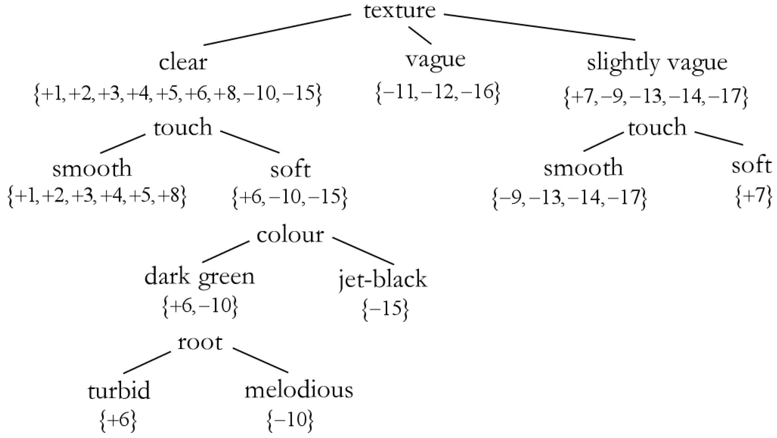
3.5. Calculation Example
4. Experiments and Result Analysis
4.1. Experimental Environment
4.2. Algorithm Comparison Experiment
- (1)
- Comparison of classification accuracy
- (2)
- Error analysis
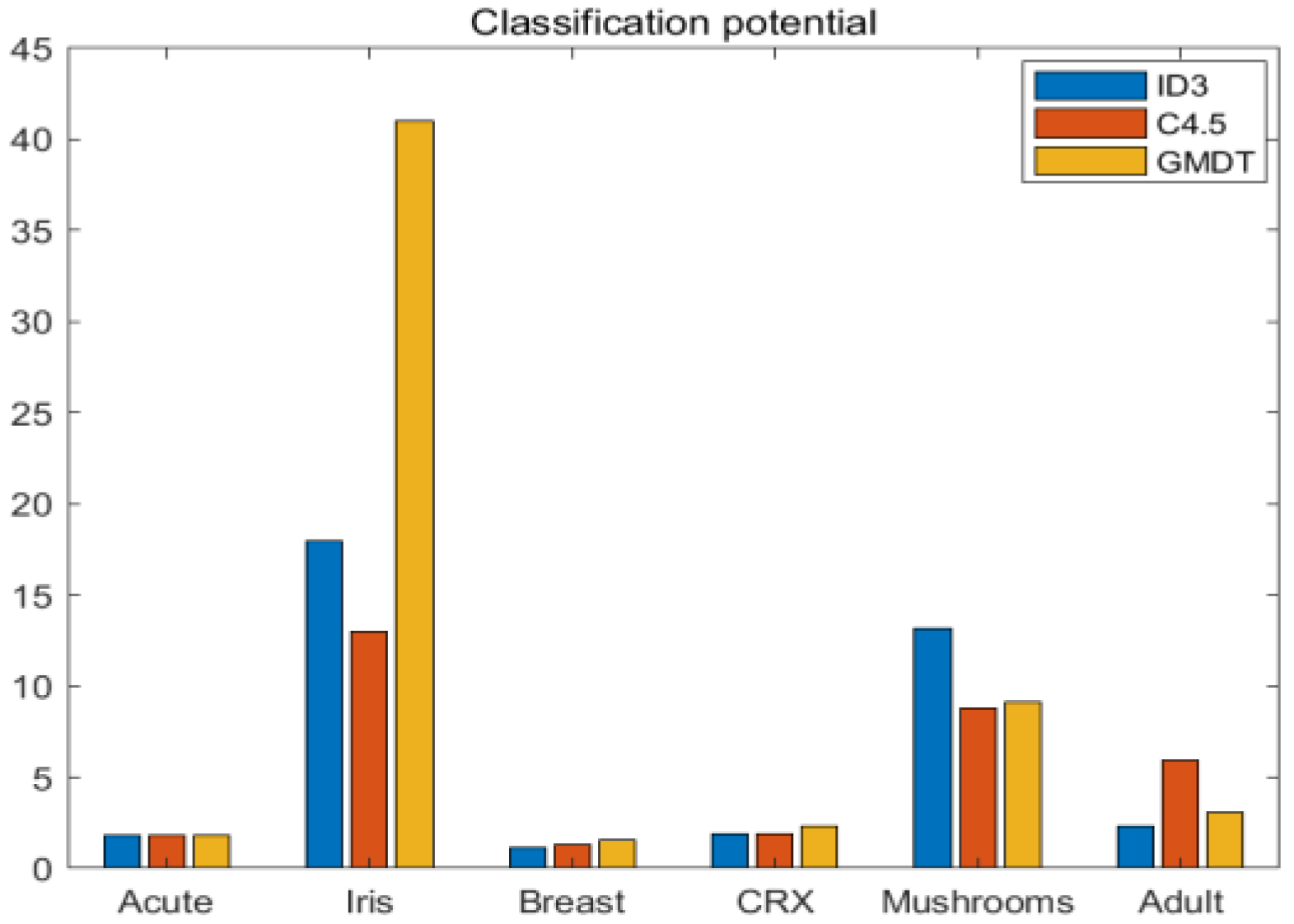
- (3)
- Comparison of classification potential
5. Conclusions
Author Contributions
Funding
Data Availability Statement
Acknowledgments
Conflicts of Interest
References
- Fu, C. Research on Data Classification Algorithm Based on Granular Computing. Ph.D. Thesis, Dalian University of Technology, Dalian, China, 2021. [Google Scholar]
- Zhang, C.L.; Zhang, L. A New ID3 Algorithm Based on Revised Information Gain. Comput. Eng. Sci. 2008, 30, 46–47. [Google Scholar]
- Jin, C.; Luo, D.-L.; Mu, F.-X. An improved ID3 decision tree algorithm. In Proceedings of the 2009 4th International Conference on Computer Science & Education, Nanning, China, 25–28 July 2009; pp. 127–130. [Google Scholar]
- Breiman, L.; Friedman, J.H.; Olshen, R.A.; Stone, C.J. Classification and Regression Trees; Routledge: Oxford, UK, 2017. [Google Scholar]
- Prasad, L.V.; Naidu, M.M. CC-SLIQ: Performance Enhancement with 2k Split Points in SLIQ Decision Tree Algorithm. IAENG Int. J. Comput. Sci. 2014, 41, 163–173. [Google Scholar]
- Wei, H.N. Research on Parallel Decision Tree Classification Based on SPRINT Method. Comput. Appl. 2005, 39–41. [Google Scholar]
- Chandra, B.; Varghese, P.P. Fuzzy SLIQ decision tree algorithm. IEEE Trans. Syst. Man Cybern. Part B 2008, 38, 1294–1301. [Google Scholar] [CrossRef]
- Honglei, G.; Changqian, M.; Wenjian, W. Model decision tree algorithm for multicore Bayesian optimization. J. Natl. Univ. Def. Technol. 2022, 44, 67–76. [Google Scholar]
- Yun, J.; Seo, J.W.; Yoon, T. Fuzzy decision tree. Int. J. Fuzzy Log. Syst. 2014, 4. [Google Scholar] [CrossRef]
- Bujnowski, P.; Szmidt, E.; Kacprzyk, J. An approach to intuitionistic fuzzy decision trees. In Proceedings of the 2015 Conference of the International Fuzzy Systems Association and the European Society for Fuzzy Logic and Technology (IFSA-EUSFLAT-15), Asturias, Spain, 30 June–3 July 2015; pp. 1253–1260. [Google Scholar]
- Yu, B.; Guo, L.; Li, Q. A characterization of novel rough fuzzy sets of information systems and their application in decision making. Expert Syst. Appl. 2019, 122, 253–261. [Google Scholar] [CrossRef]
- Marudi, M.; Ben-Gal, I.; Singer, G. A decision tree-based method for ordinal classification problems. IISE Trans. 2022, 1–15. [Google Scholar] [CrossRef]
- Wang, Y. An ordered decision tree algorithm based on fuzzy dominant complementary mutual information. Comput. Appl. 2021, 41, 2785–2792. [Google Scholar]
- Zhao, H.; Wang, P.; Hu, Q.; Zhu, P.; Xu, J.; Fang, H.; Zhou, T.; Chen, Y.-H.; Guo, H.; Zeng, F. Fuzzy rough set based feature selection for large-scale hierarchical classification. IEEE Trans. Fuzzy Syst. 2019, 27, 1891–1903. [Google Scholar] [CrossRef]
- Tawhid, M.A.; Ibrahim, A.M. Feature selection based on rough set approach, wrapper approach, and binary whale optimization algorithm. Int. J. Mach. Learn. Cybern. 2020, 11, 573–602. [Google Scholar] [CrossRef]
- Yue, Y.; Xian, Z.; Shuai, C. Decision tree induction algorithm based on attribute purity. Comput. Eng. Des. 2021, 42, 142–149. [Google Scholar]
- Wang, R.; Liu, Z.; Ji, J. Decision tree algorithm based on attribute importance. Comput. Sci. 2017, 44, 129–132. [Google Scholar]
- Xie, X.; Zhang, X.Y.; Yang, J.L. A decision tree algorithm incorporating information gain and Gini index. Comput. Eng. Usage 2022, 58, 139–144. [Google Scholar]
- Wu, S.B.; Chen, C.G.; Huang, R. ID3 optimization algorithm based on correlation coefficient. Comput. Eng. Sci. 2016, 38, 2342–2347. [Google Scholar]
- Choi, S.H.; Shin, J.M.; Choi, Y.H. Dynamic nonparametric random forest using covariance. Secur. Commun. Netw. 2019, 2019, 1–12. [Google Scholar] [CrossRef]
- Kozak, J. Decision Tree and Ensemble Learning Based on Ant Colony Optimization; Springer International Publishing: Berlin/Heidelberg, Germany, 2019. [Google Scholar]
- Mu, Y.; Liu, X.; Yang, Z.; Liu, X. A parallel C4. 5 decision tree algorithm based on MapReduce. Concurr. Comput. Pract. Exp. 2017, 29, e4015. [Google Scholar] [CrossRef]
- Liang, J.; Qian, Y.; Li, D.; Hu, Q. Research progress on theory and method of granular computing for big data. Big Data 2016, 2, 13–23. [Google Scholar]
- Miao, D.; Hu, S. Uncertainty analysis based on granular computing. J. Northwest Univ. 2019, 49, 487–495. [Google Scholar]
- Khazali, N.; Sharifi, M.; Ahmadi, M.A. Application of fuzzy decision tree in EOR screening assessment. J. Pet. Sci. Eng. 2019, 177, 167–180. [Google Scholar] [CrossRef]
- Rabcan, J.; Rusnak, P.; Kostolny, J.; Stankovic, R. Comparison of algorithms for fuzzy decision tree induction. In Proceedings of the 2020 18th International Conference on Emerging eLearning Technologies and Applications (ICETA), Kosice, Slovenia, 12–13 November 2020; pp. 544–551. [Google Scholar]
- Zhang, K.; Zhan, J.; Wu, W.Z. Novel fuzzy rough set models and corresponding applications to multi-criteria decision-making. Fuzzy Sets Syst. 2020, 383, 92–126. [Google Scholar] [CrossRef]
- Qian, W.; Huang, J.; Wang, Y.; Xie, Y. Label distribution feature selection for multi-label classification with rough set. Int. J. Approx. Reason. 2021, 128, 32–55. [Google Scholar] [CrossRef]
- Chen, C.E.; Ma, X. Information system rule extraction method based on granular computing. J. Northwest Norm. Univ. 2018, 54, 11–15. [Google Scholar]
- Wu, J.; Wang, C. Multidimensional granular matrix correlation analysis for big data and applications. Comput. Sci. 2017, 44, 407–410+421. [Google Scholar]
- Pawlak, Z. Rough sets. Int. J. Comput. Inf. Sci. 1982, 11, 341–356. [Google Scholar] [CrossRef]
- Miao, Z.; Li, D. Rough Set Theory Algorithms and Applications; Tsinghua University Press: Beijing, China, 2008. [Google Scholar]
- Yang, J.; Wang, G.; Zhang, Q. Evaluation model of rough grain structure based on knowledge distance. J. Intell. Syst. 2020, 15, 166–174. [Google Scholar]
- Yang, J.; Wang, G.; Zhang, Q. Similarity metrics for multi-granularity cloud models. Pattern Recognit. Artif. Intell. 2018, 31, 677–692. [Google Scholar]
- Qian, Y.; Liang, J.; Dang, C. Knowledge structure, knowledge granulation and knowledge distance in a knowledge base. Int. J. Approx. Reason. 2009, 50, 174–188. [Google Scholar] [CrossRef]
- Zhou, R.; Jin, J.; Cui, Y.; Ning, S.; Bai, X.; Zhang, L.; Zhou, Y.; Wu, C.; Tong, F. Agricultural drought vulnerability assessment and diagnosis based on entropy fuzzy pattern recognition and subtraction set pair potential. Alex. Eng. J. 2022, 61, 51–63. [Google Scholar] [CrossRef]


| U | C | D | ||
|---|---|---|---|---|
| Color | Price | Size | Buy | |
| 1 | White | High | Full | No |
| 2 | White | Low | Compact | Yes |
| 3 | Black | Low | Compact | No |
| 4 | Black | Low | Full | Yes |
| 5 | Grey | High | Full | Yes |
| 6 | Grey | High | Compact | No |
| U | C | D | |||||
|---|---|---|---|---|---|---|---|
| Color | Root | Stroke | Texture | Umbilical | Touch | Good | |
| 1 | D-green | Curl up | Turbid | Clear | Depressed | Smooth | Yes |
| 2 | Jet-black | Curl up | Dull | Clear | Depressed | Smooth | Yes |
| 3 | Jet-black | Curl up | Turbid | Clear | Depressed | Smooth | Yes |
| 4 | D-green | Curl up | Dull | Clear | Depressed | Smooth | Yes |
| 5 | Plain | Curl up | Turbid | Clear | Depressed | Smooth | Yes |
| 6 | D-green | Slightly curl | Turbid | Clear | Concave | Soft | Yes |
| 7 | Jet-black | Slightly curl | Turbid | S-vague | Concave | Soft | Yes |
| 8 | Jet-black | Slightly curl | Turbid | Clear | Concave | Smooth | Yes |
| 9 | Jet-black | Slightly curl | Dull | S-vague | Concave | Smooth | No |
| 10 | D-green | Stiff | Melodious | Clear | Flat | Soft | No |
| 11 | Plain | Stiff | Melodious | Vague | Flat | Smooth | No |
| 12 | Plain | Curl up | Turbid | Vague | Flat | Soft | No |
| 13 | D-green | Slightly curl | Turbid | S-vague | Depressed | Smooth | No |
| 14 | Plain | Slightly curl | Dull | S-vague | Depressed | Smooth | No |
| 15 | Jet-black | Slightly curl | Turbid | Clear | Concave | Soft | No |
| 16 | Plain | Curl up | Turbid | Vague | Flat | Smooth | No |
| 17 | D-green | Curl up | Dull | S-vague | Concave | Smooth | No |
| No. | Dataset | Samples | Attributes | Class |
|---|---|---|---|---|
| 1 | Acute Inflammations | 121 | 6 | 2 |
| 2 | Iris | 151 | 4 | 3 |
| 3 | Breast Cancer | 286 | 9 | 2 |
| 4 | CRX | 654 | 15 | 2 |
| 5 | Mushrooms | 8125 | 21 | 2 |
| 6 | Adult | 32,561 | 14 | 2 |
| No. | Data | Classification Accuracy | ||
|---|---|---|---|---|
| ID3 | C4.5 | GMDT | ||
| 1 | Acute Inflammations | 0.64 | 0.64 | 0.64 |
| 2 | Iris | 0.80 | 0.87 | 0.90 |
| 3 | Breast Cancer | 0.46 | 0.53 | 0.61 |
| 4 | CRX | 0.31 | 0.34 | 0.63 |
| 5 | Mushrooms | 0.80 | 0.87 | 0.90 |
| 6 | Adult | 0.27 | 0.45 | 0.75 |
| No. | Data | Error Analysis | ||
|---|---|---|---|---|
| ID3 | C4.5 | GMDT | ||
| 1 | Acute Inflammations | (23, 0, 13) | (23, 0, 13) | (23, 0, 13) |
| 2 | Iris | (36, 7, 2) | (39, 3, 3) | (41, 3, 1) |
| 3 | Breast Cancer | (35, 10, 31) | (40, 6, 30) | (46, 0, 30) |
| 4 | CRX | (64, 110, 34) | (70, 101, 37) | (131, 20, 57) |
| 5 | Mushrooms | (1950, 340, 148) | (2126, 168, 144) | (2197, 0, 241) |
| 6 | Adult | (2679, 5937, 1153) | (4396, 4662, 738) | (7352, 33, 2384) |
Disclaimer/Publisher’s Note: The statements, opinions and data contained in all publications are solely those of the individual author(s) and contributor(s) and not of MDPI and/or the editor(s). MDPI and/or the editor(s) disclaim responsibility for any injury to people or property resulting from any ideas, methods, instructions or products referred to in the content. |
© 2023 by the authors. Licensee MDPI, Basel, Switzerland. This article is an open access article distributed under the terms and conditions of the Creative Commons Attribution (CC BY) license (https://creativecommons.org/licenses/by/4.0/).
Share and Cite
Meng, L.; Bai, B.; Zhang, W.; Liu, L.; Zhang, C. Research on a Decision Tree Classification Algorithm Based on Granular Matrices. Electronics 2023, 12, 4470. https://doi.org/10.3390/electronics12214470
Meng L, Bai B, Zhang W, Liu L, Zhang C. Research on a Decision Tree Classification Algorithm Based on Granular Matrices. Electronics. 2023; 12(21):4470. https://doi.org/10.3390/electronics12214470
Chicago/Turabian StyleMeng, Lijuan, Bin Bai, Wenda Zhang, Lu Liu, and Chunying Zhang. 2023. "Research on a Decision Tree Classification Algorithm Based on Granular Matrices" Electronics 12, no. 21: 4470. https://doi.org/10.3390/electronics12214470
APA StyleMeng, L., Bai, B., Zhang, W., Liu, L., & Zhang, C. (2023). Research on a Decision Tree Classification Algorithm Based on Granular Matrices. Electronics, 12(21), 4470. https://doi.org/10.3390/electronics12214470