Experiments were conducted in a structured manner to evaluate the performance of the ASViS algorithm in comparison to conventional methods. Each investigation was targeted towards elucidating specific attributes and behaviors. The performance of ASViS is influenced by several specific parameters, which will be elaborated upon in the subsequent sections. Notably, network conditions, such as , packet loss, and buffer conditions, have been identified. Additionally, variations in parameters across different layers and alterations in the size of each layer have been observed to impact performance. A thorough examination of these factors and their implications on ASViS functionality is included in the following discussions. The first experiment juxtaposed a theoretical model of ASViS, particularly in assessing the anticipated arrival time of frames at the client side, against an empirical counterpart. The purpose was to determine the accuracy of the theoretical model in simulating network dynamics. The second experiment delved into the perceived video quality by modulating the parameter . By setting a continuum of equidistant benchmarks, the Y-PSNR was gauged, revealing a complex interrelation between the values and the Y-PSNR attained. In the third analysis, the objective was to discern the optimal curfew gaps, represented as the set of taus, suitable for static initial network scenarios. Here, the MM method paved the way to unearthing superior video quality. Unlike assuming uniform curfew gaps, this study hypothesized better outcomes from distinct-sized intervals, with the Y-PSNR being the primary metric of evaluation. The fourth exploration sought to validate the theory that layer-based deadline gaps echo the proportions of the layer sizes. The culminating experiment instituted a face-off between two ABR protocols, ASViS and MPC. Using a spectrum of metrics, from VB behavior and throughput to video quality, this comparative study decoded the operational nuances of ASViS juxtaposed with the MPC algorithm.
5.1. Results
The objective of the first experiment is to compare the network behavior outcomes of a theoretical ASViS model with those of an experimental test. Both scenarios employ UDP transmission rules equipped with flow control to prevent congestion. In the theoretical model, the determination of which packets are discarded is based on the Estimated Packet Size (EPS) and network conditions as utilized by the ASViS algorithm. The EPS values are informed by the mean layer size information derived from a trace file, which is created for JSVM. The size in
for each layer is presented in
Table 2. For the experimental model, the actual size of each layer, influenced by its content, whether it is BL or EL, and its classification as I or B, is utilized. This results in a variety of sizes for each layer. The size in [kB] for each layer is presented in
Table 2. Both models operate with the same network transmission parameters:
0.05 s, packet loss rate 0.01, and buffer 3 s. Results are calculated based on 100 pseudo-random seeds.
Within the ASViS model, the behavior can shift from conservative to risky by adjusting the
values. For a video comprising four layers, it might be presumed that there would be four distinct
values representing BI, BB, EI, and EB. However, in this experiment, the
value for the
layer is set at 0 due to its importance. This ensures its transmission until the deadline is reached. Seven configurations, each with an equidistant and incremental
gap (
G) based on layer priorities, are outlined in
Table 3.
The results, both theoretical and experimental, appear in
Figure 6. This representation showcases the estimated arrival time of each frame at the client end. The gradient of the slope conveys the transmission rate; a gentler slope indicates a higher rate, whereas a steeper one suggests a slower rate. A significant gap between theoretical and experimental results is observed for
. This discrepancy can be attributed to various factors, including differences in average vs. actual packet size and video complexity variations.
To determine the accuracy of the correlation between models, the Mean Absolute Percentage Error (MAPE) is employed.
Table 4 provides a detailed breakdown, pointing out a maximum prediction error of approximately 14.2% for
. Given the inherent variability of the practical experiments due to packet losses and the intricate characteristics of each frame, along with the nuances of the various layers and complexities associated with network conditions in empirical analyses, the accuracy of the theoretical model is underscored. It is noteworthy that high fidelity is achieved by the theoretical model, aligning well with the experimental results. This contributes to a reduction in the need for exhaustive and computationally demanding empirical tests, thereby facilitating more streamlined behavioral predictions based on the theoretical model. It is important to stress that this does not replace empirical benchmarks but can significantly reduce the amount of energy, resources, and time devoted to more practical tests.
The aim of the second experiment is to analyze how the video quality performance of ASViS is influenced by varying
values, placing emphasis on the experimental outcomes. The network transmission parameters for this investigation are as follows:
0.05 s, packet loss rate 0.01, and buffer 1 s. Results are calculated based on 100 pseudo-random seeds for each
. The configuration of
adheres to the format provided in
Table 3. This study also assesses the behavior of SVC in the absence of ASViS, termed the “no protocol” condition.
Figure 7 delineates the arrival time at the client side against each frame for every specified
. The scenario devoid of a protocol displays results closely aligned with the deadline. Nevertheless, the Y-PSNR performance for each
is illustrated in
Figure 8. This representation indicates superior performance in the “no protocol” scenario. It is also observed that there exists a significant correlation between increased
and decreased Y-PSNR.
At an initial assessment, it may be surmised that SVC without ASViS offers superior results. However, upon closer analysis, this assumption is challenged. One primary objective of ABR algorithms is the prevention of rebuffering. Data presented in
Figure 9, which portray the fluctuation in VB size relative to video playout, reveal stalls occurring after the 50% playout in scenarios lacking a protocol. In situations with ASViS, there are no observable stalls for any
, and a rise in the VB size is witnessed as the
value increases.
In the third experiment, the objective is to pinpoint optimal values to maximize specific criteria. For this experiment, the optimization objective is the performance of ASViS, based on the average amount of sent layer outcomes, using the MM method. It is crucial to note that these optimal values might not always be integers, suggesting a broad range of potential values. The foundational setup for this experiment involved fixed parameters such as an of 0.05 s, a packet loss rate of 1/200, and a buffer of 1 s. For BI, a fixed value of at 0 s (representing the deadline) was applied. In contrast, for the layers BB, EI, and EB, the values , , and were adjusted, respectively. Performance was evaluated based on the maximum number of layers transmitted, with a combined limit of 300 layers: 19 for BI, 19 for EI, 141 for BB, and 141 for EB. This evaluation determined the local maxima within each quadrant. For each point, ten pseudo-random seeds were probed, and the average of the maximums was obtained. A consistent search range, spanning from 0 to 8 s, was employed for each .
The visualization of these results is provided in a 3D plot, as seen in
Figure 10. The axes, labeled as
,
, and
, represent the Gaps (G) or intervals between consecutive
values, excluding
. These represent the intervals from the deadline to
, from
to
, and finally from
to
. It is crucial to recognize that these intervals are sequential and do not intersect. The overall time span between the deadline and
is the collective sum of
,
, and
. Based on the fixed conditions of the
and packet loss, optimal performance metrics were identified as
0
,
0
,
1
, and
2
for the layers BI, BB, EI, and EB, respectively.
For experiment 4, a hypothesis was formulated stating that the gaps in layered-based deadlines (represented by
values) are dependent on and proportional to the layer sizes. The video detailed in
Table 1 features relatively small base layers and large enhancement layers due to quantization in each layer. To test this hypothesis, the configuration was reversed (i.e., small enhancement layers and large base layers) for testing purposes, and the network conditions from experiment 3 were used. The same three-dimensional maximum value search using the MM method was then performed. The details of each Layer Size Configuration (LSC) can be found in
Table 5. This table represents the average accumulated size per layer in a GOP structure of IB × 7.
corresponds to experiment 3, while
is the same video from
Table 1 but with a quantization of 20 for both BL and EL.
Performance, based on the percentage of sent layer outcomes and derived using the MM method for
, is presented in
Figure 11. A preliminary comparison of the two 3D coordinates results,
Figure 10 and
Figure 11, reveals significant differences in the optimal
values between the two LSCs. Detailed coordinates, referencing
,
, and
, are provided in
Table 6.
A thorough examination of the results between
and
, and the corresponding layer sizes, has revealed a distinct association between the
values and the sizes of layers. As depicted in
Figure 12, the normalized layer sizes and the
values for scenarios
and
are juxtaposed. It has been discerned from the blue markers that layer 2 holds a predominant role in both configurations. Conversely, the red markers have indicated that elevated
values are associated with more diminutive layers. A noticeable inverse correlation between the layer sizes and
values is evident: as the magnitude of a layer amplifies, the optimal
for video quality is observed to wane. The pivotal influence of layer sizes on video quality, in the context of
, is underscored by this relationship.
In the fifth experiment, a comparison was made between the performance of the ABR algorithms, MPC and ASViS, using various parameters. Traditional TCP behavior, which is typical for ABR algorithms, was exhibited under the network conditions for MPC. In contrast, User Datagram Protocol (UDP) with flow control was employed by ASViS, consistent with previous experiments. Network transmission parameters from experiment 3 were replicated, and the values for the ASViS protocol were derived from the same experiment. A total of 100 simulations were executed for both ABR algorithms, and the results presented were the mean values obtained from all simulations.
A chunk size of 4 GOP was designated for MPC, equivalent to 32 frames or roughly 1 s of playout, given a frame rate of 30 fps. Four bitrate levels, labeled as
R, were used, each integrating various layers. Comprehensive details of each
R can be accessed in
Table 7. An average across all chunks served as a reference for AVQ of Y-PSNR in this MPC implementation, accompanied by a chunk size (
) specified in bits. The initial
spanned from 0.1 s to 5 s, incremented by 0.2 s. The estimated throughput (
C) was calculated as the harmonic mean throughput of the previous five chunks, with weight assignments of
,
, and
, aligning with the recommendations in [
49].
As illustrated in
Figure 13, the relationship between the VB size variation and video playout was mapped. Results indicated that a mean VB size of 1.5 s with a standard deviation of 0.5 s was achieved by MPC, whereas ASViS achieved a mean of 0.45 s with a deviation of 0.08 s. Notably, greater stability after 20% of video playout was observed with ASViS, despite its reduced mean VB size.
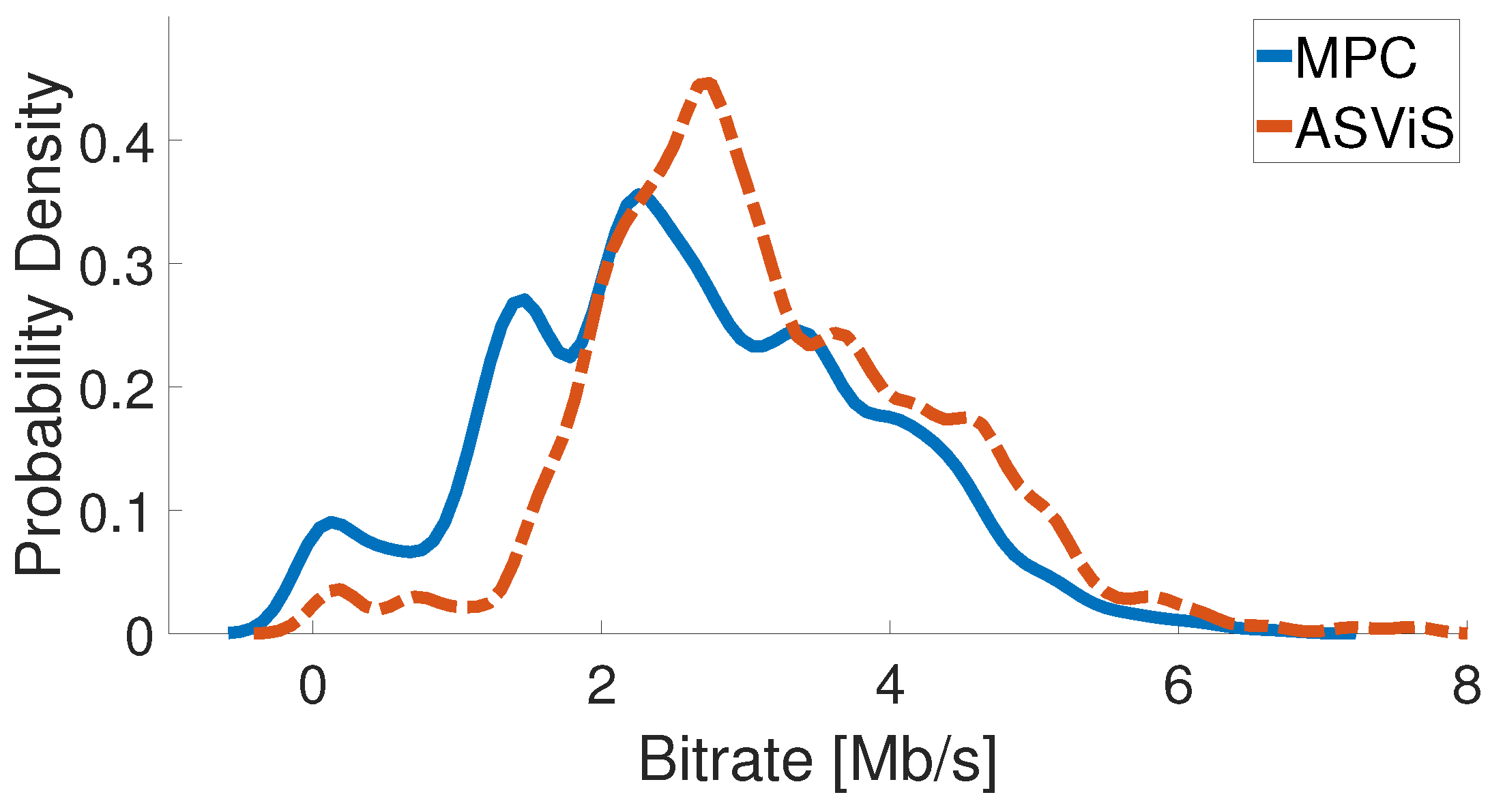
Figure 14 portrays the anticipated bitrate distribution for both MPC and ASViS. This visualization aids in comprehending the adaptability of each algorithm to network conditions. An in-depth analysis confirmed that the bitrate estimated distribution for ASViS predominantly focuses on values higher than those for MPC, a pattern that contrasts with its mean and standard deviation provided in
Table 8.
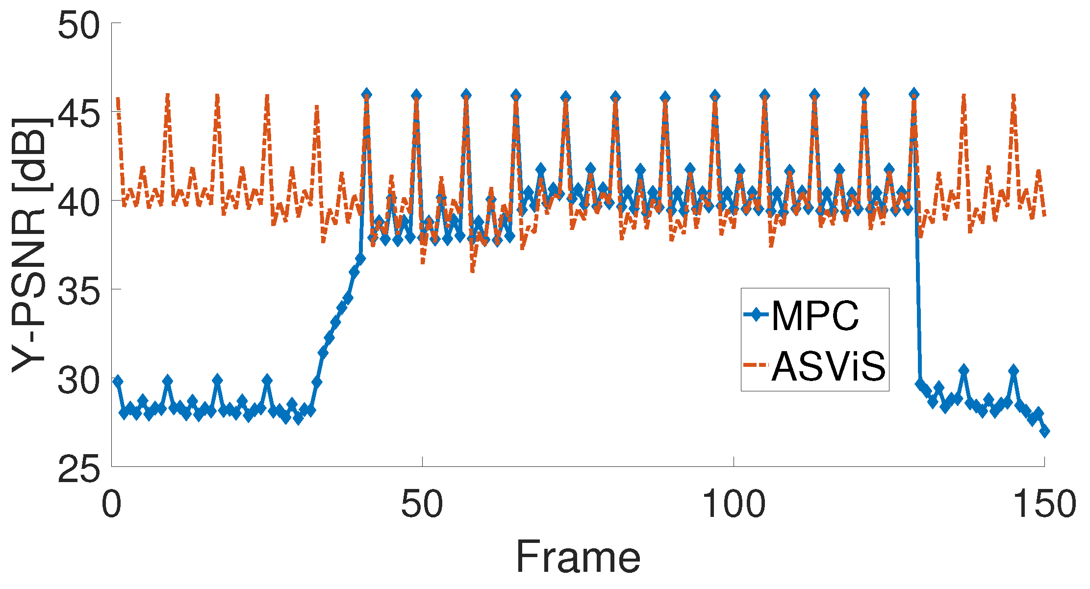
Subsequent evaluations explored video quality throughout the entire video playback. The Y-PSNR findings are presented in
Figure 15, whereas VMAF results can be found in
Figure 16. Both algorithms exhibited comparable video quality from frames 40 to 130. However, at the commencement and conclusion of the video playback, the quality of MPC was observed to be inferior to that of ASViS. This discrepancy is attributed to the conservative approach of MPC and its slower adaptation to network conditions compared to ASViS.
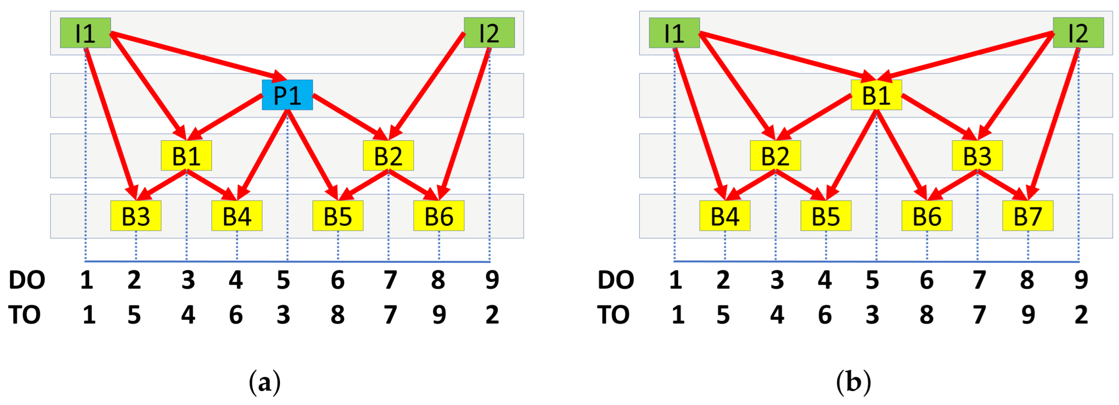
Furthermore, a noteworthy distinction between the results of frames 74 and 84 was observed in
Figure 16, owing to the capability of VMAF to discern details overlooked by Y-PSNR. Detailed analysis revealed that frames 74 and 84, corresponding to a B4 frame as cross-referenced with
Figure 1b, were dropped by ASViS.
The video quality metrics, presented in
Figure 15 and
Figure 16, were analyzed using a distinctive approach involving a boxplot and its corresponding histogram. The boxplot delineates the median, the 25th percentile at the bottom, and the 75th percentile at the top. Whiskers extend to cover values not deemed outliers. Notably, since no outliers were observed, there are no ‘+’ markers. The results for Y-PSNR and VMAF are displayed in
Figure 17 and
Figure 18, respectively. Although Y-PSNR and VMAF are founded on different philosophies, both metrics consistently show the superiority of ASViS over MPC. For a comprehensive understanding of the mean and deviation values of Y-PSNR, VMAF, and bitrate, one can refer to
Table 8. It becomes evident that, in terms of VMAF, Y-PSNR, and bitrate, the ASViS algorithm holds an edge over MPC.
5.2. Discussion
The initial experiment demonstrates a close alignment between theoretical and observed behaviors of ASViS, with mean absolute percentage errors ranging between 6.5% and 14.2%. These findings substantiate the capability of the model to predict the experimental behavior of ASViS, thus eliminating the need for time-consuming emulations or tests.
Outcomes of the second experiment indicate superior video quality in a no-protocol scenario (default SVC) compared to any gap configuration scenario. However, this scenario exhibits video stalls, with rebuffering incidents accounting for over half the video playback duration. In contrast, all scenarios display variations in video buffering without complete depletion. Video quality can vary based on configuration, offering insights into how ASViS modulates video quality to ensure uninterrupted playback.
The third experiment leverages the MM method to discern specific coordinates that yield improved video quality under given network conditions. It reveals that optimal video quality can span a broad range of values and might be envisioned as a multi-dimensional solution. In the fourth experiment, a pronounced inverse correlation is found between the values and layer sizes. This discovery is pivotal, suggesting that service providers can sidestep the task of pinpointing optimal values for individual videos. They can instead modify layer deadlines in proportion to layer sizes, ensuring nearly optimal outcomes.
Findings of the fifth experiment spotlight the superiority of ASViS over MPC in multiple aspects. ASViS records a 5.8% and 4.6% higher Y-PSNR and VMAF, respectively, than MPC. Moreover, ASViS displays a consistently compact video buffer size compared to MPC. It also boasts more efficient network utilization, with a bitrate surpassing that of MPC, and steadier performance, reflected in a reduced standard deviation. In conclusion, these promising results position ASViS as a skillful ABR algorithm.
While the potential of ASViS has been demonstrated in specific contexts through our experiments, its performance in broader or more challenging scenarios remains an intriguing area of speculation. In 5G mobile networks, known for high download speeds and reduced latency, it is hypothesized that ASViS could deliver ultra-high-definition video streaming with minimal interruptions. Conversely, in regions with underdeveloped internet infrastructure or in satellite networks with inherent high latency, challenges may arise regarding how ASViS adapts video flow and manages fluctuations. It might be theorized that smooth but lower-quality video playback could prevail. Further research is warranted in these areas. Future directions are aimed at exploring and validating these scenarios to ensure the resilience of ASViS beyond ideal conditions. For future directions, it is proposed that more exhaustive tests be conducted, involving videos with varying resolutions and different frame rates. Additionally, it has been identified that simulations need to be carried out under realistic network conditions, such as those of mobile networks.


