

Analysis of High-Frequency Communication Channel Characteristics in a Typical Deep-Sea Incomplete Sound Channel

Abstract
:1. Introduction
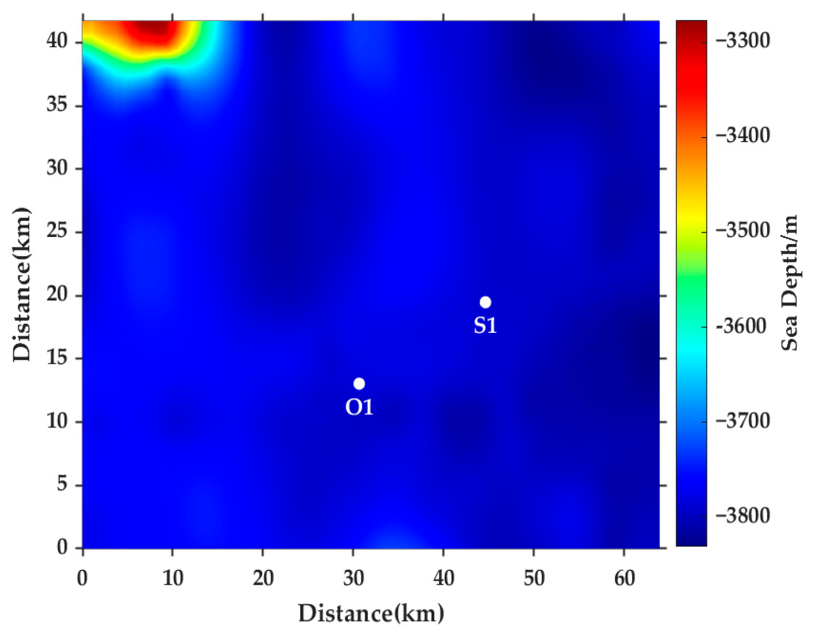
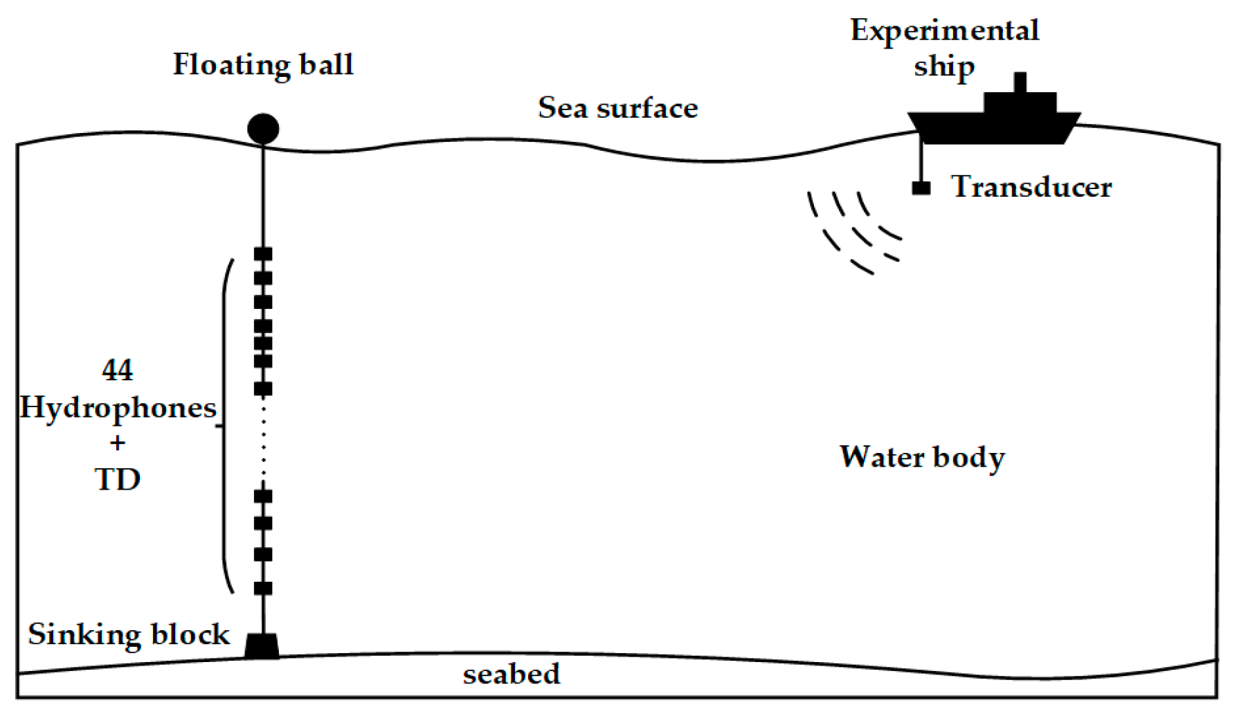
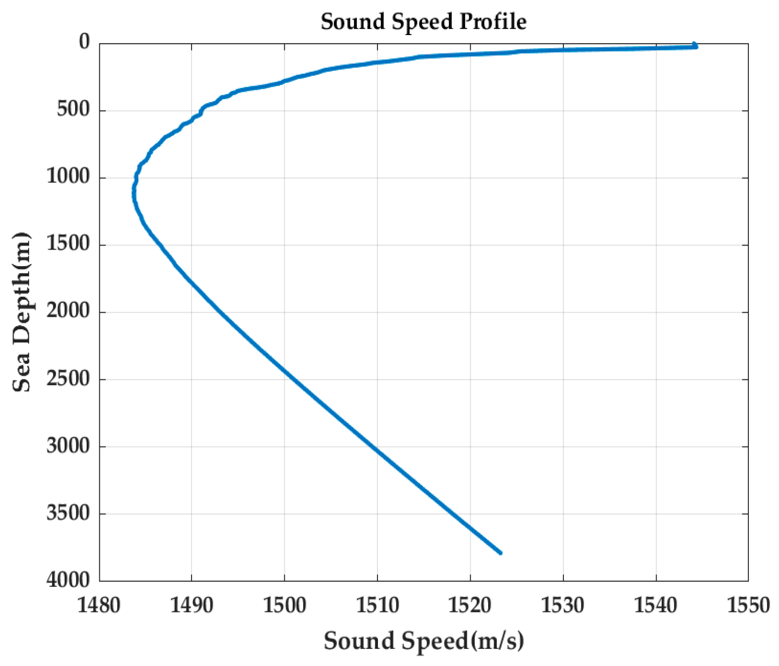
2. Overview of the Experiment
3. Underwater Acoustics Channel Statistics
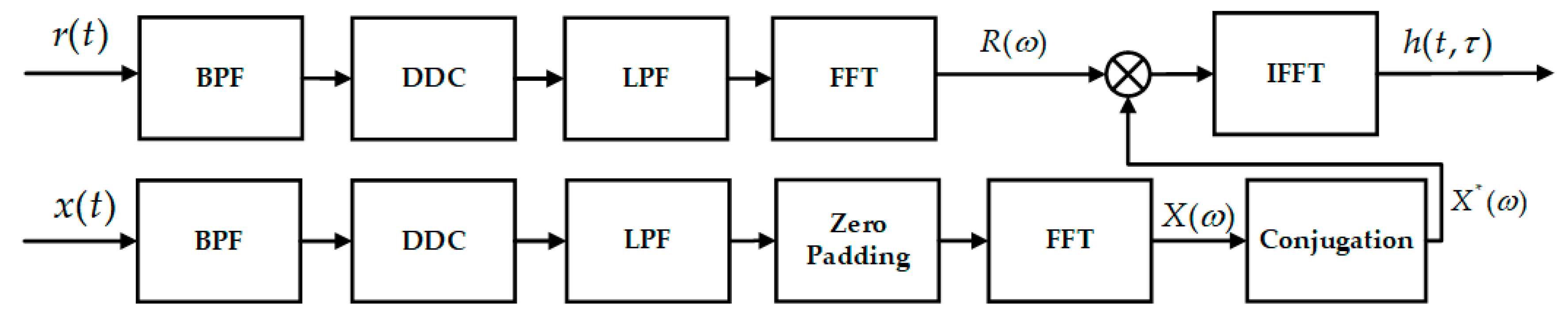
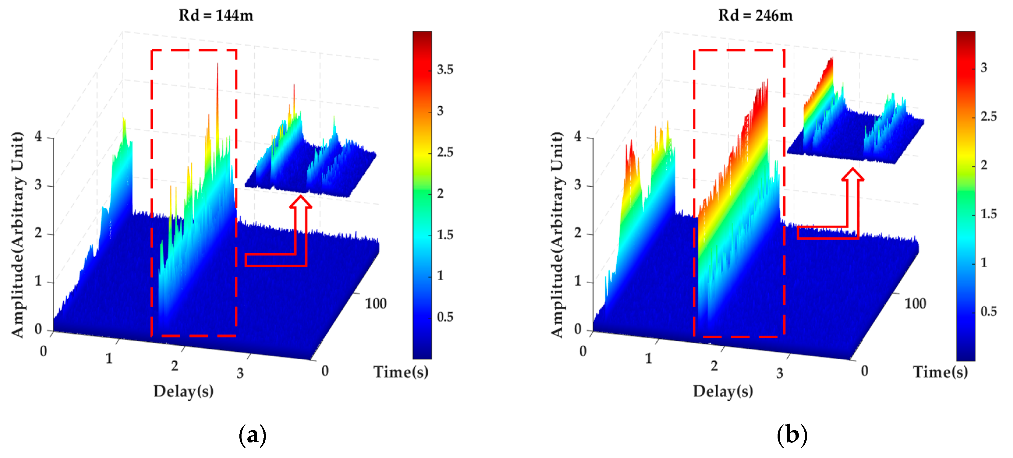
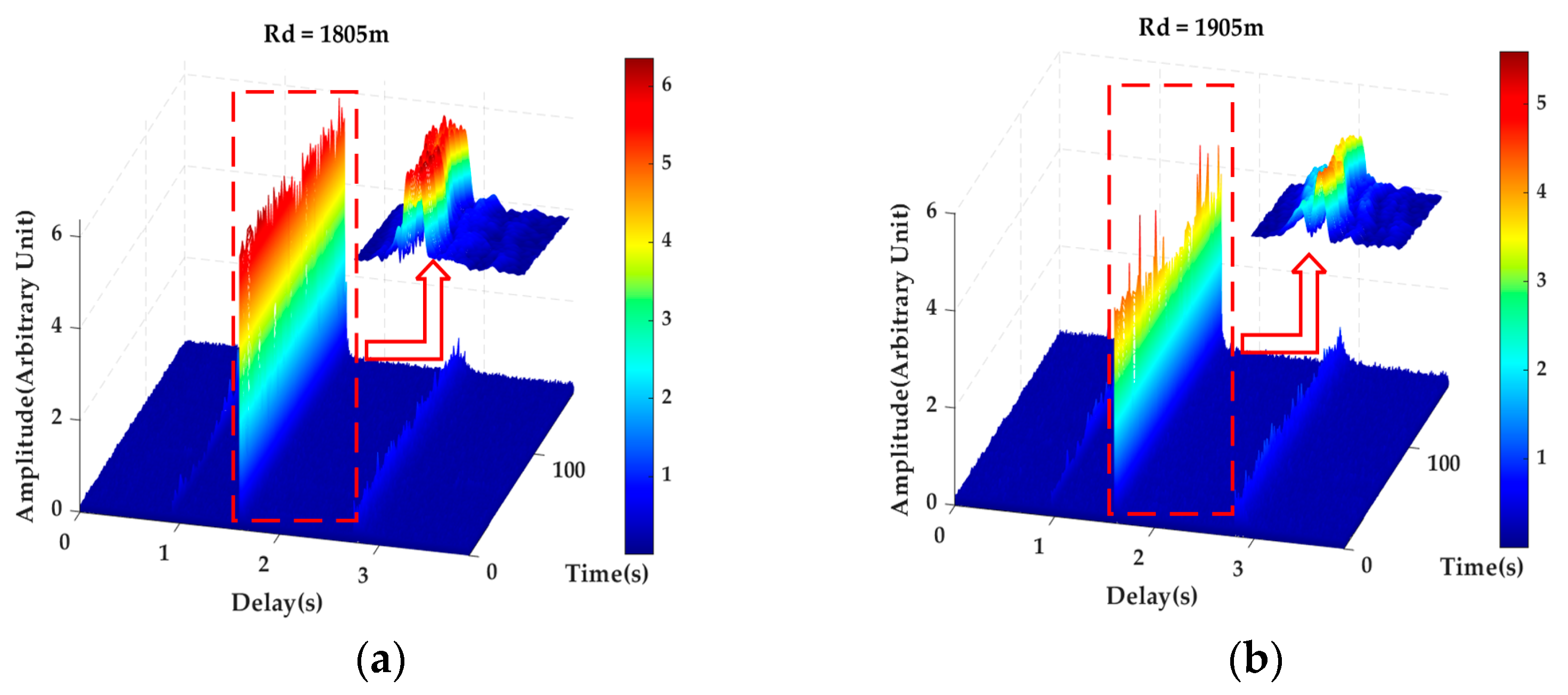
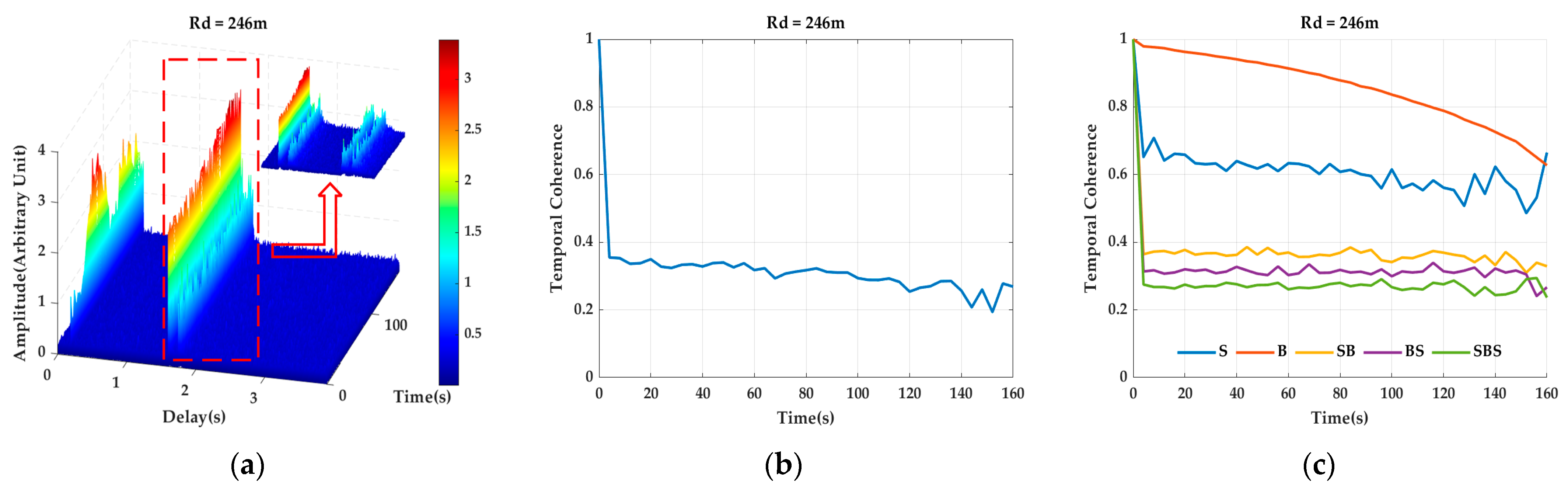
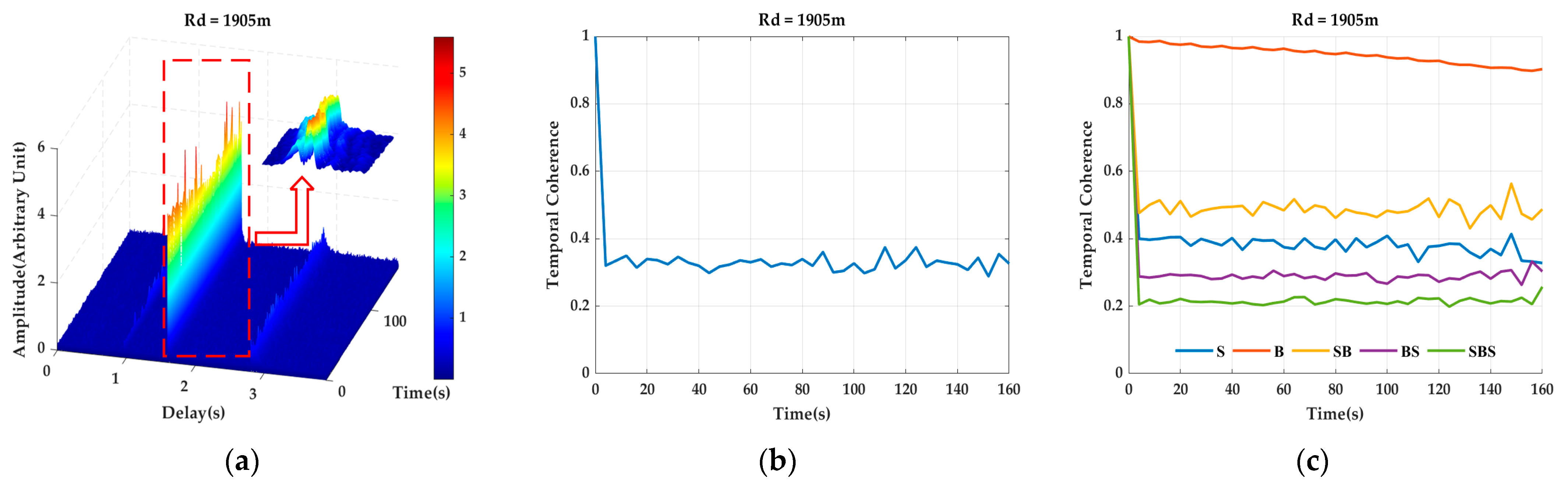
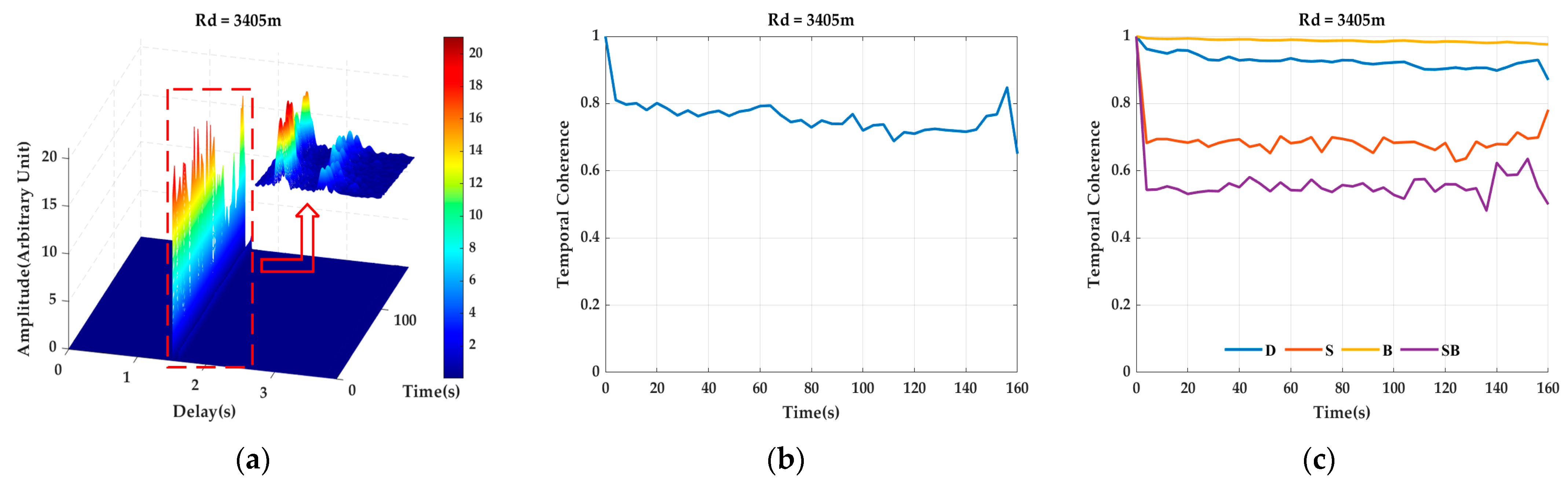
3.1. CIR
3.2. Cluster Amplitude and Coefficient of Variation
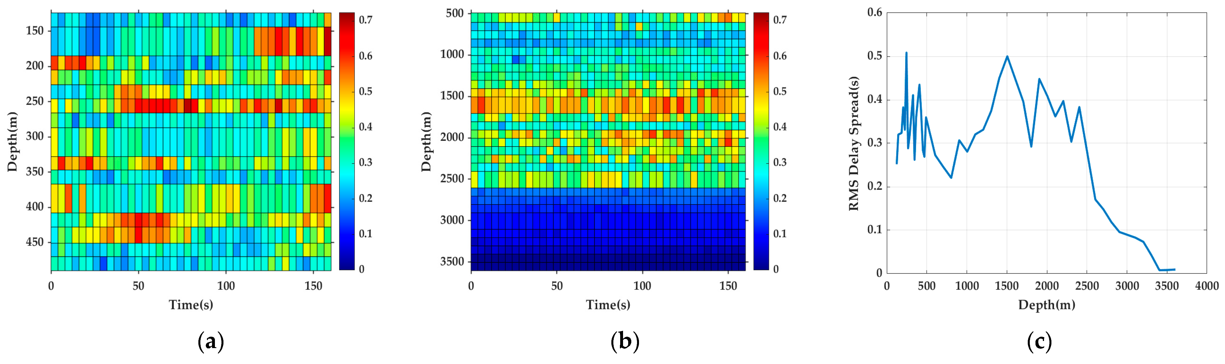
3.3. RMS Delay Spread
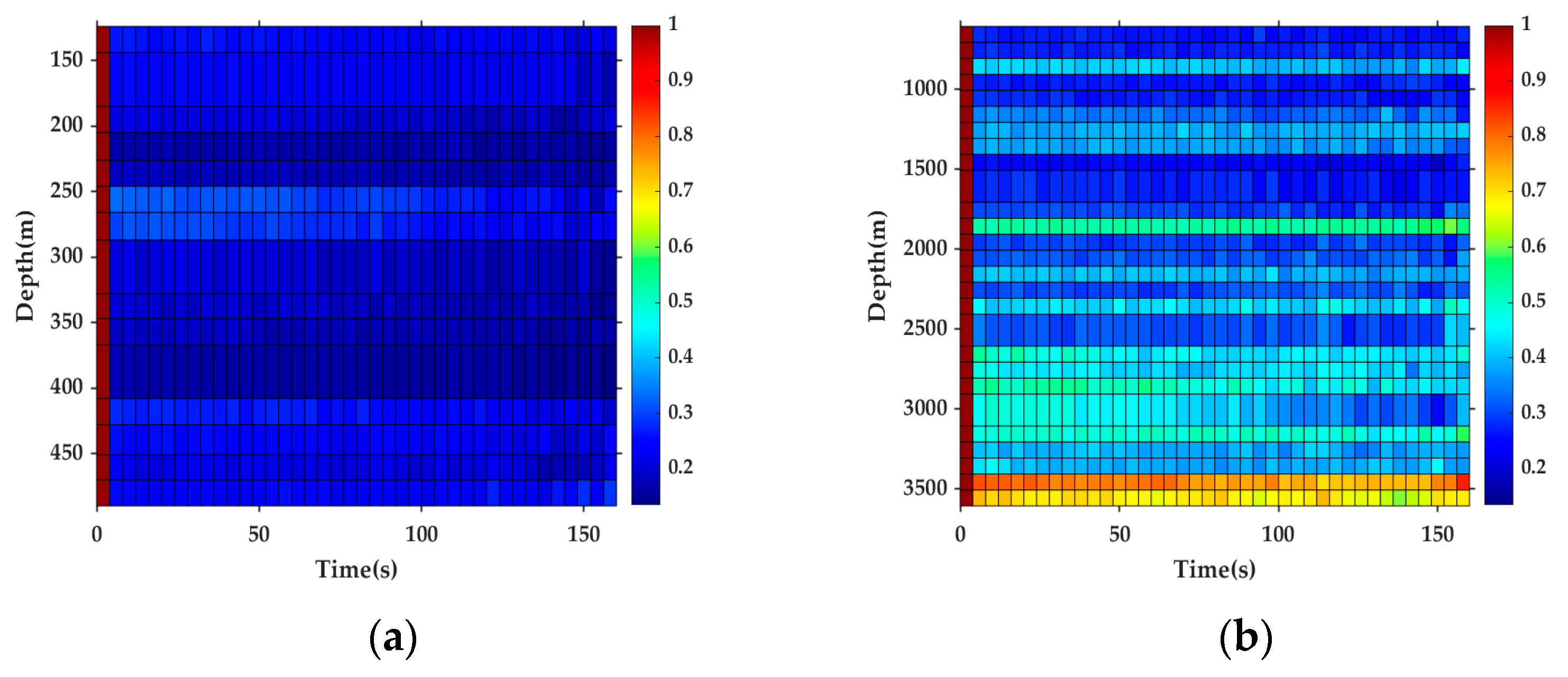
3.4. Temporal Coherence Coefficient
4. Analysis of the Experiment Data
4.1. Vertical Structure Change in Channel
4.2. Coefficient of Variation of the Cluster Amplitudes
4.3. RMS Delay Spread
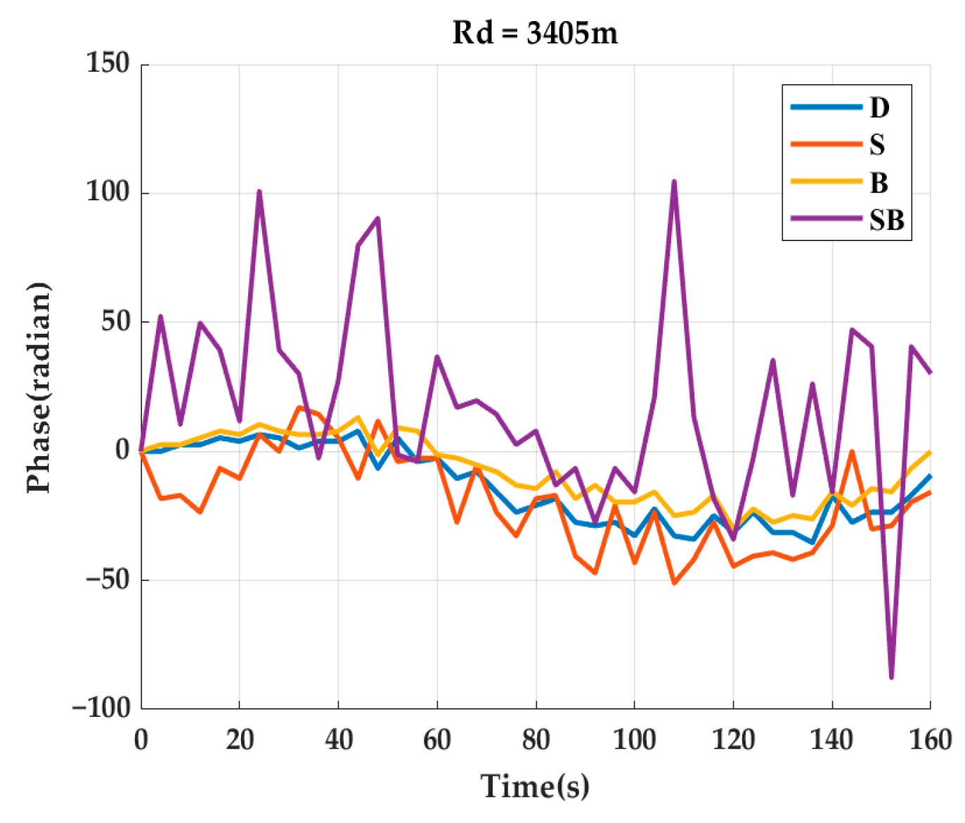
4.4. Channel Temporal Coherence and Cluster Analysis
5. Conclusions
6. Future Work
Author Contributions
Funding
Data Availability Statement
Acknowledgments
Conflicts of Interest
Abbreviations
| Abbreviation | Full Name |
| RMS | Root mean square |
| CIR | Channel impulse response |
| LFM | Linear frequency modulation |
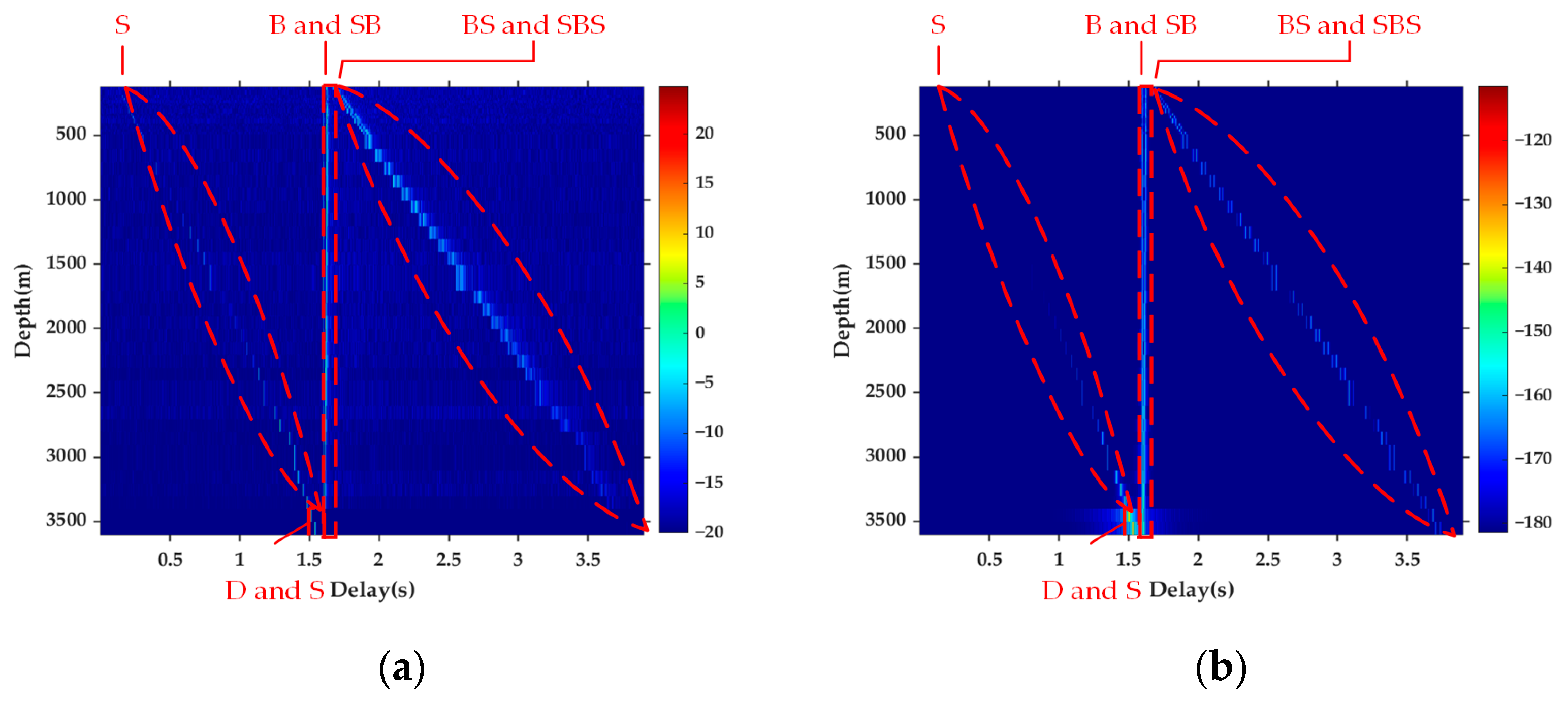
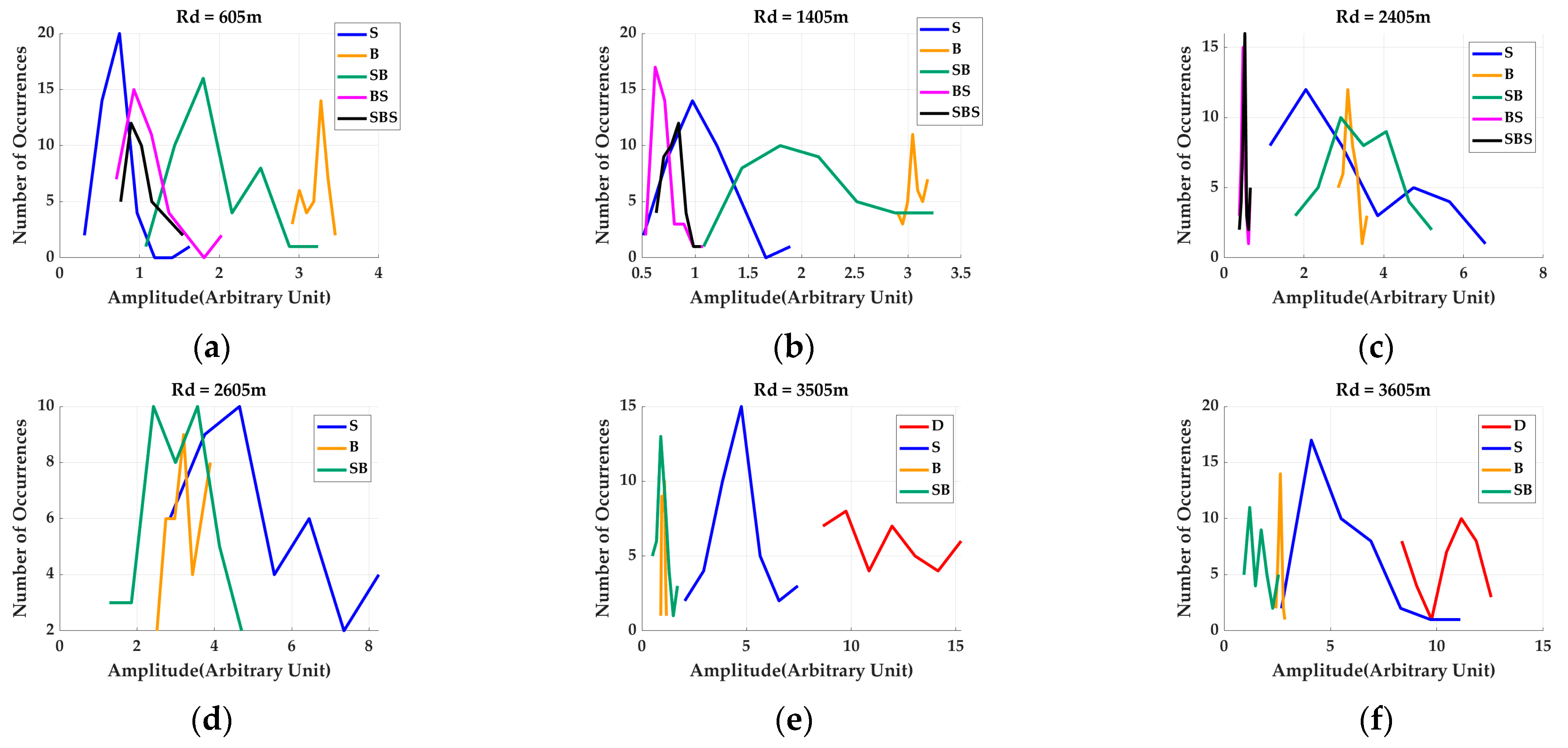
| D | Direct path cluster |
| S | Surface path cluster |
| B | Bottom path cluster |
| SB | Surface–bottom path cluster |
| BS | Bottom–surface path cluster |
| SBS | Surface–bottom–surface path cluster |
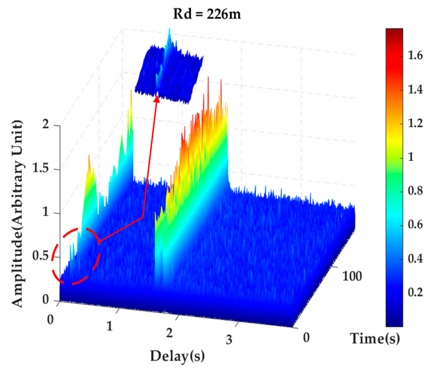
| Rd | Receiving depth |
References
- Stojanovic, M.; Preisig, J. Underwater Acoustic Communication Channels: Propagation Models and Statistical Characterization. IEEE Commun. Mag. 2009, 47, 84–89. [Google Scholar] [CrossRef]
- Stojanovic, M. Underwater Acoustic Communications: Design Considerations on the Physical Layer. In Proceedings of the 2008 Fifth Annual Conference on Wireless on Demand Network Systems and Services, Garmisch-Pertenkirchen, Germany, 23–25 January 2008; pp. 1–10. [Google Scholar]
- Duda, T.F. Modeling Weak Fluctuations of Undersea Telemetry Signals. IEEE J. Ocean. Eng. 1991, 16, 3–11. [Google Scholar] [CrossRef]
- Sing, A.C.; Nelson, J.K.; Kozat, S.S. Signal Processing for Underwater Acoustic Communications. IEEE Commun. Mag. 2009, 47, 90–96. [Google Scholar] [CrossRef]
- Galvin, R.; Coats, R.E.W. A Stochastic Underwater Acoustic Channel Model. In Proceedings of the OCEANS 96 MTS/IEEE Conference Proceedings, The Coastal Ocean—Prospects for the 21st Century, Fort Lauderdale, FL, USA, 23–26 September 1996; Volume 1, pp. 203–210. [Google Scholar]
- Chitre, M. A High-Frequency Warm Shallow Water Acoustic Communications Channel Model and Measurements. J. Acoust. Soc. Am. 2007, 122, 2580. [Google Scholar] [CrossRef] [PubMed]
- Socheleau, F.-X.; Passerieux, J.-M.; Laot, C. Characterisation of Time-Varying Underwater Acoustic Communication Channel with Application to Channel Capacity. In Proceedings of the Underwater Acoustic Measurements: Technologies and Results, Nafplion, Greece, 21–26 June 2009. [Google Scholar]
- Kim, S.-M.; Byun, S.-H.; Kim, S.-G.; Lim, Y.-K. Experimental Analysis of Statistical Properties of Underwater Channel in a Very Shallow Water Using Narrow and Broadband Signals. In Proceedings of the OCEANS 2009, Biloxi, MS, USA, 26–29 October 2009; pp. 1–4. [Google Scholar]
- Radosevic, A.; Proakis, J.G.; Stojanovic, M. Statistical Characterization and Capacity of Shallow Water Acoustic Channels. In Proceedings of the OCEANS 2009-EUROPE, Bremen, Germany, 11–14 May 2009; pp. 1–8. [Google Scholar]
- Qarabaqi, P.; Stojanovic, M. Statistical Characterization and Computationally Efficient Modeling of a Class of Underwater Acoustic Communication Channels. IEEE J. Ocean. Eng. 2013, 38, 701–717. [Google Scholar] [CrossRef]
- Yang, T.C. Properties of Underwater Acoustic Communication Channels in Shallow Water. J. Acoust. Soc. Am. 2012, 131, 129–145. [Google Scholar] [CrossRef] [PubMed]
- Qarabaqi, P.; Stojanovic, M. Modeling the Large Scale Transmission Loss in Underwater Acoustic Channels. In Proceedings of the 2011 49th Annual Allerton Conference on Communication, Control, and Computing (Allerton), Monticello, IL, USA, 28–30 September 2011; pp. 445–452. [Google Scholar]
- Tomasi, B.; Casari, P.; Badia, L.; Zorzi, M. A Study of Incremental Redundancy Hybrid ARQ over Markov Channel Models Derived from Experimental Data. In Proceedings of the Fifth ACM International Workshop on UnderWater Networks—WUWNet ’10, Woods Hole, MA, USA, 30 September–1 October 2010; pp. 1–8. [Google Scholar]
- Wang, Y.; Yan, H.; Pan, C.; Liu, S. Measurement-Based Analysis of Characteristics of Fast Moving Underwater Acoustic Communication Channel. In Proceedings of the 2022 International Conference on Frontiers of Information Technology (FIT), Islamabad, Pakistan, 12–13 December 2022; pp. 47–52. [Google Scholar]
- Yang, W.-B.; Yang, T.C. High-Frequency Channel Characterization for M-Ary Frequency-Shift-Keying Underwater Acoustic Communications. J. Acoust. Soc. Am. 2006, 120, 2615–2626. [Google Scholar] [CrossRef]
- Zuo, M.; Tu, X.; Yang, S.; Fang, H.; Wen, X.; Qu, F. Channel Distribution and Noise Characteristics of Distributed Acoustic Sensing Underwater Communications. IEEE Sens. J. 2021, 21, 24185–24194. [Google Scholar] [CrossRef]
- Santoso, T.B.; Widjiati, E.; Wirawan; Hendrantoro, G. The Evaluation of Probe Signals for Impulse Response Measurements in Shallow Water Environment. IEEE Trans. Instrum. Meas. 2016, 65, 1292–1299. [Google Scholar] [CrossRef]
- Walree, P.V. Channel Sounding for Acoustic Communications: Techniques and Shallow-Water Examples. Available online: http://hdl.handle.net/20.500.12242/2456 (accessed on 7 August 2023).
- Wang, Y.; Wang, C.-X.; Zhu, X.; He, Y.; Chang, H.; Sun, J.; Zhang, W. A 3D Non-Stationary GBSM for Mobile-to-Mobile Underwater Acoustic Communication Channels. In Proceedings of the 2021 IEEE/CIC International Conference on Communications in China (ICCC), Xiamen, China, 28–30 July 2021; pp. 511–516. [Google Scholar]
- Fan, C.; Wei, L.; Wang, Z. Adaptive Switching for Communication Profiles in Underwater Acoustic Modems Based on Reinforcement Learning. In Proceedings of the 16th International Conference on Underwater Networks & Systems, Boston, MA, USA, 14–16 November 2022; pp. 1–7. [Google Scholar]
- Yang, T.C. Temporal Coherence of Sound Transmissions in Deep Water Revisited. J. Acoust. Soc. Am. 2008, 124, 113–127. [Google Scholar] [CrossRef]
- Zhou, Y.; Song, A.; Tong, F. Underwater Acoustic Channel Characteristics and Communication Performance at 85 kHz. J. Acoust. Soc. Am. 2017, 142, EL350–EL355. [Google Scholar] [CrossRef]
- Huang, S.H.; Yang, T.C.; Huang, C.-F. Multipath Correlations in Underwater Acoustic Communication Channels. J. Acoust. Soc. Am. 2013, 133, 2180–2190. [Google Scholar] [CrossRef] [PubMed]
- Huang, S.H.; Tsao, J.; Yang, T.C.; Cheng, S.-W. Model-Based Signal Subspace Channel Tracking for Correlated Underwater Acoustic Communication Channels. IEEE J. Ocean. Eng. 2014, 39, 343–356. [Google Scholar] [CrossRef]
- Sadanandan, P.; Sameer Babu, T.P.; Neena, K.A. Measurement and Characterization of Long Range Stationary and Short Range Mobile Underwater Wireless Acoustic Channels. In Proceedings of the 2014 Fourth International Conference on Advances in Computing and Communications, Rohtak, India, 8–9 February 2014; pp. 239–242. [Google Scholar]
- Tsimenidis, C.C.; Sharif, B.S.; Hinton, O.R.; Adams, A.E. Analysis and Modelling of Experimental Doubly-Spread Shallow-Water Acoustic Channels. Eur. Ocean. 2005, 2, 854–858. [Google Scholar]
- Liu, B.; Jia, N.; Huang, J.; Guo, S.; Xiao, D.; Ma, L. Autoregressive Model of an Underwater Acoustic Channel in the Frequency Domain. Appl. Acoust. 2022, 185, 108397. [Google Scholar] [CrossRef]
- Porter, M.B.; Bucker, H.P. Gaussian Beam Tracing for Computing Ocean Acoustic Fields. J. Acoust. Soc. Am. 1987, 82, 1349–1359. [Google Scholar] [CrossRef]
- Jensen, F.B.; Kuperman, W.A.; Porter, M.B.; Schmidt, H. Computational Ocean Acoustics; Modern Acoustics and Signal Processing; Springer: New York, NY, USA, 2011. [Google Scholar] [CrossRef]


| Environmental Parameters | Value |
|---|---|
| Frequency range (kHz) | 8–12 |
| Transmitter depth (m) | 44.8 |
| Range between transmitter and receiver (km) | 14.8 |
| Receiver depth (m) | 124–3605 |
| Sea depth (m) | 3790 |
| Rd (m) | D | S | B | SB | BS | SBS |
|---|---|---|---|---|---|---|
| 605 | 0.186 | 1 | 0.521 | 0.350 | 0.303 | |
| 1405 | 0.219 | 1 | 0.574 | 0.241 | 0.246 | |
| 2405 | 0.549 | 0.858 | 1 | 0.168 | 0.162 | |
| 2605 | 0.804 | 1 | 0.880 | 0.054 | 0.039 | |
| 3505 | 1 | 0.460 | 0.118 | 0.084 | 0.008 | 0.007 |
| 3605 | 1 | 0.561 | 0.222 | 0.100 | 0.009 | 0.008 |
| Rd (m) | D | S | B | SB | BS | SBS |
|---|---|---|---|---|---|---|
| 605 | 0.328 | 0.047 | 0.258 | 0.284 | 0.202 | |
| 1405 | 0.270 | 0.029 | 0.278 | 0.160 | 0.121 | |
| 2405 | 0.492 | 0.063 | 0.256 | 0.156 | 0.137 | |
| 3105 | 0.434 | 0.060 | 0.334 | |||
| 3505 | 0.193 | 0.274 | 0.061 | 0.330 | ||
| 3605 | 0.132 | 0.333 | 0.034 | 0.314 |
| Sound Field Zone | Different Characteristics | Same Characteristics |
|---|---|---|
| Shadow zone | 1. The channel path clusters contained B and SB and may have contained S, BS, and SBS. 2. The channel RMS delay spread ranged from 0.1 s to 0.6 s. 3. The channel temporal coherence ranged from 0.2 to 0.6. | 1.The coefficients of variation of the path clusters related to the sea surface were high (>0.1). On the contrary, the coefficient of variation of B was low (<0.1). 2. The temporal coherence of B was much higher than that of other path clusters, and the temporal coherence of sea-related path clusters was very low. 3. The phase fluctuation of B was smaller than that of other path clusters. |
| Direct-arrival zone | 1. The channel path clusters contained D, S, B, and SB. The energy of BS and SBS was negligible. 2. The channel RMS delay spread was less than 0.1 s 3. The channel temporal coherence ranged from 0.6 to 0.8. |
Disclaimer/Publisher’s Note: The statements, opinions and data contained in all publications are solely those of the individual author(s) and contributor(s) and not of MDPI and/or the editor(s). MDPI and/or the editor(s) disclaim responsibility for any injury to people or property resulting from any ideas, methods, instructions or products referred to in the content. |
© 2023 by the authors. Licensee MDPI, Basel, Switzerland. This article is an open access article distributed under the terms and conditions of the Creative Commons Attribution (CC BY) license (https://creativecommons.org/licenses/by/4.0/).
Share and Cite
Li, Y.; Jia, N.; Huang, J.; Han, R.; Guo, Z.; Guo, S. Analysis of High-Frequency Communication Channel Characteristics in a Typical Deep-Sea Incomplete Sound Channel. Electronics 2023, 12, 4562. https://doi.org/10.3390/electronics12224562
Li Y, Jia N, Huang J, Han R, Guo Z, Guo S. Analysis of High-Frequency Communication Channel Characteristics in a Typical Deep-Sea Incomplete Sound Channel. Electronics. 2023; 12(22):4562. https://doi.org/10.3390/electronics12224562
Chicago/Turabian StyleLi, Yunfei, Ning Jia, Jianchun Huang, Ruigang Han, Zhongyuan Guo, and Shengming Guo. 2023. "Analysis of High-Frequency Communication Channel Characteristics in a Typical Deep-Sea Incomplete Sound Channel" Electronics 12, no. 22: 4562. https://doi.org/10.3390/electronics12224562
APA StyleLi, Y., Jia, N., Huang, J., Han, R., Guo, Z., & Guo, S. (2023). Analysis of High-Frequency Communication Channel Characteristics in a Typical Deep-Sea Incomplete Sound Channel. Electronics, 12(22), 4562. https://doi.org/10.3390/electronics12224562